

Thermal Degradation of Carboxymethyl Cellulose (CMC) in Saline Solution for Applications in Petroleum Industry Fluids
 , ,
, ,
Abstract
1. Introduction
2. Materials and Methods
2.1. Materials
2.2. Methods
2.2.1. Characterization of CMC Powders
2.2.2. Characterizations of CMC Solutions at Room Temperature
2.2.3. Exposure to Temperature of Saline Solution (SSW)
3. Results and Discussion
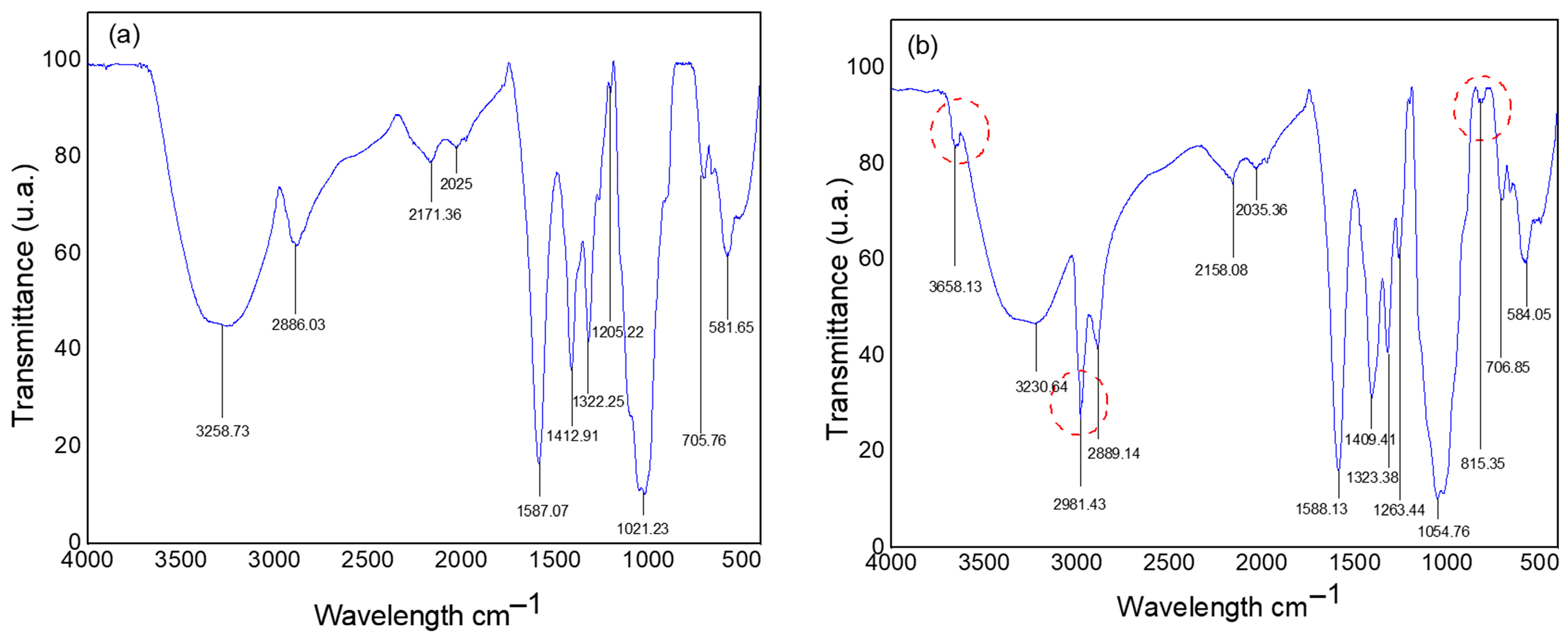
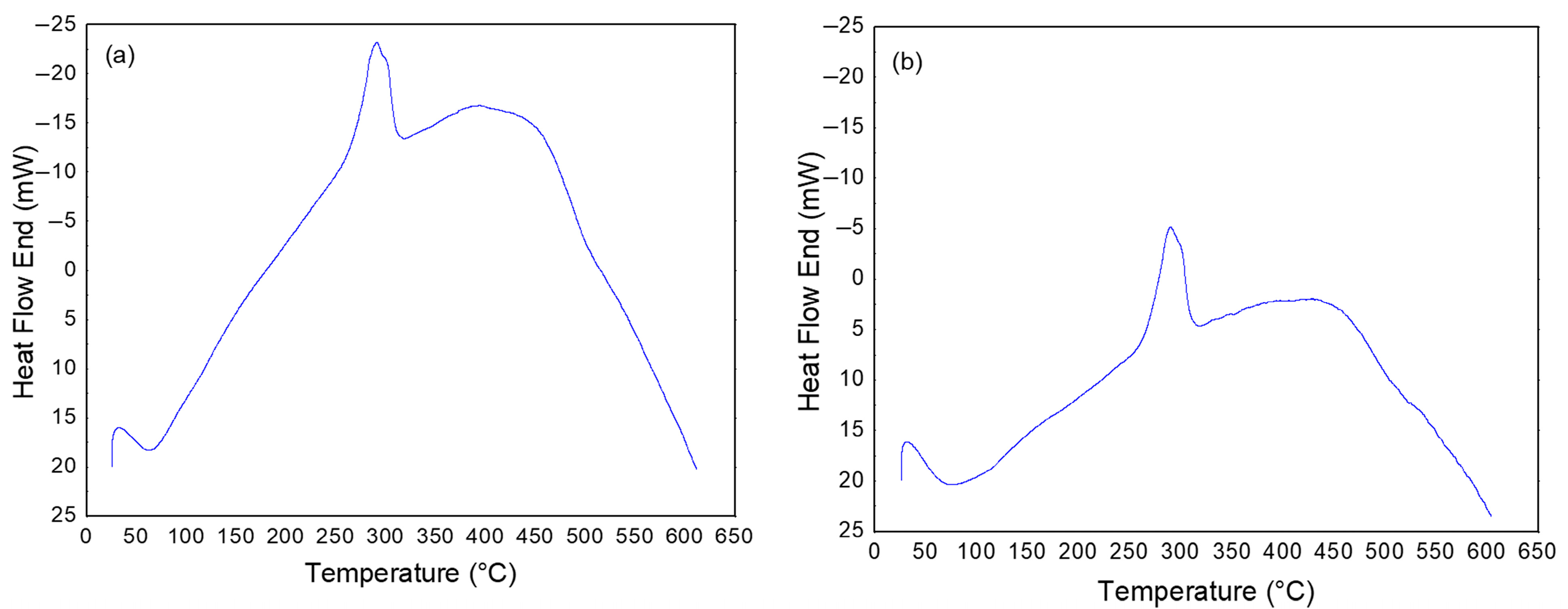
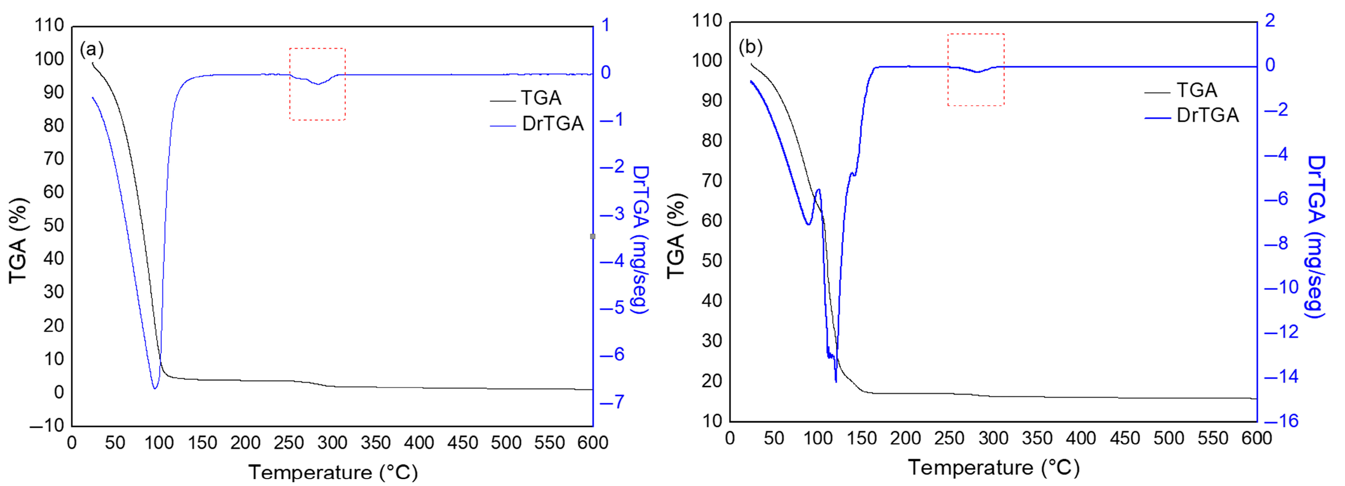
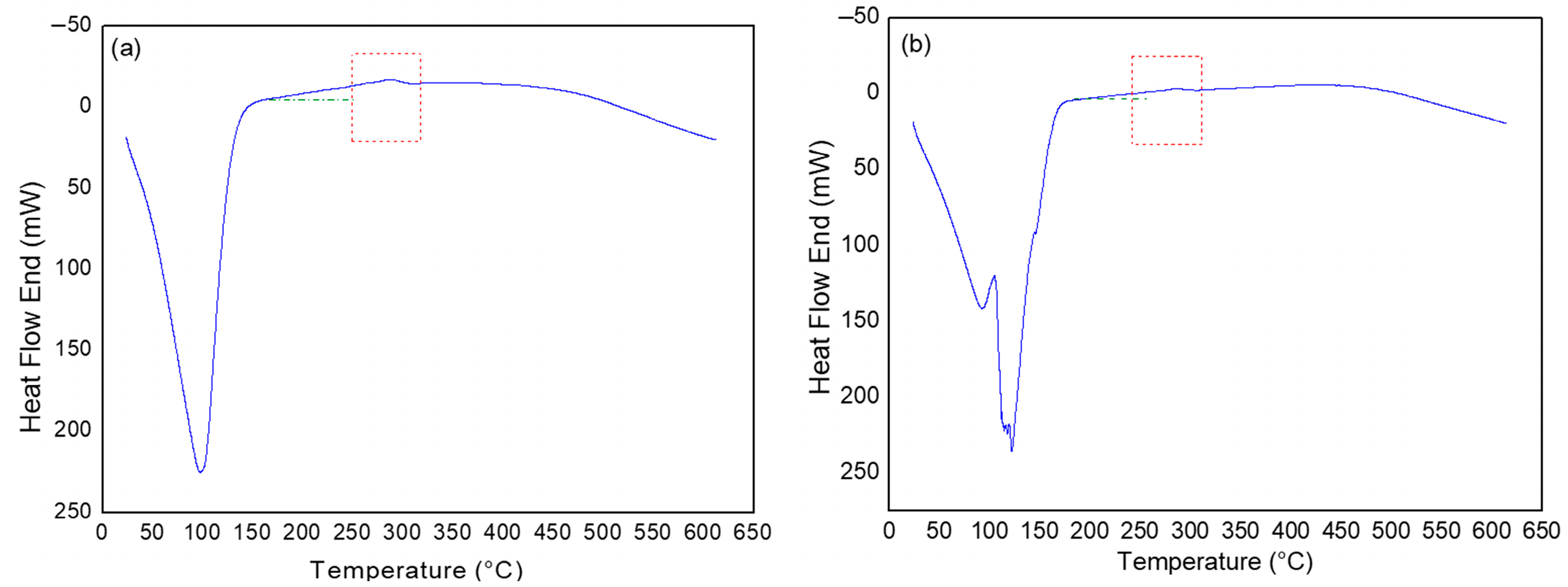
3.1. Characterization of CMC Powders
3.2. Characterization of CMC Solutions at Room Temperature
3.3. Characterization of Saline Solution (SSW) After Exposure to Temperature
4. Conclusions
- There are no significant differences between the morphological and thermal characteristics of CMC LV and CMC HV in the powder state;
- The interaction of CMC with the salt present in solution has no significant influence on thermal degradation, but it directly influences the rheological behavior of the solution at room temperature;
- The SSW solution, composed of CMC LV and CMC HV solubilized in brine, remained thermally stable after exposure to conditions of 70 °C/24 h, 70 °C/12 h, and 110 °C/48 h, but it underwent total degradation at 150 °C/24 h and 150 °C/72 h;
- CMC LV and CMC HV, used together in saline solutions, may compromise the rheological behavior, even if there is no thermal degradation of the polymers, so that significant reductions in the viscosity values of the solutions are observed for temperatures above 110 °C.
Author Contributions
Funding
Data Availability Statement
Acknowledgments
Conflicts of Interest
References
- Medhi, S.; Chowdhury, S.; Dehury, R.; Khaklari, G.H.; Puzari, S.; Bharadwaj, J.; Talukdar, P.; Sangwai, J.S. Comprehensive review on the recent advancements in nanoparticle-based drilling fluids: Properties, performance, and perspectives. Energ. Fuel 2024, 38, 13455–13513. [Google Scholar] [CrossRef]
- Davoodi, S.; Al-Shargabi, M.; Wood, D.A.; Rukavishnikov, V.S.; Minaev, K.M. Synthetic polymers: A review of applications in drilling fluids. Pet. Sci. 2024, 21, 475–518. [Google Scholar] [CrossRef]
- Ahmed, A.W.; Kalkan, E. Drilling fluids: Types, formation choices and environmental impact. IJLTEMAS 2019, 8, 1–10. [Google Scholar]
- Caenn, R.; Darley, H.C.H.; Gray, G.R. Composition and Properties of Drilling and Completion Fluids, 6th ed; Gulf Professional Publishing: Houston, TX, USA, 2020. [Google Scholar]
- Peysson, Y. Solid/Liquid dispersions in drilling and production. Oil Gas Sci. Technol. 2004, 59, 11–21. [Google Scholar] [CrossRef]
- Skadsem, H.J.; Giljarhus, K.E.T.; Fredheim, F.Ø.; Riet, E.V.; Keultjes, W.J.G. Vibration-assisted annular fluid displacement for rig-less well abandonment operations. J. Pet. Sci. Eng. 2022, 215, 110717. [Google Scholar] [CrossRef]
- Akpan, E.U. Using environmentally friendly polymers as rheological control and fluid loss additives in water-based drilling muds. Geoenergy Sci. Eng. 2024, 242, 213195. [Google Scholar] [CrossRef]
- Aghdam, S.B.; Moslemizadeh, A.; Kowsari, E.; Asghari, N. Synthesis and performance evaluation of a novel polymeric fluid loss controller in water-based drilling fluids: High-temperature and high-salinity conditions. J. Nat. Gas Sci. Eng. 2020, 83, 103576. [Google Scholar] [CrossRef]
- Akpan, E.U.; Enyi, P.D.C.; Nasr, G.G. Enhancing the performance of xanthan gum in water-based mud systems using an environmentally friendly biopolymer. J. Pet. Explor. Prod. Technol. 2020, 10, 1933–1948. [Google Scholar] [CrossRef]
- Taghdimi, R.; Kaffashi, B.; Rasaei, M.R.; Dabiri, M.S.; Hemmati-Sarapardeh, A. Formulation of a new drilling mud using biopolymers, nanoparticles and SDS and investigation of its rheological behavior, interfacial tension and formation damage. Braz. J. Sci. 2023, 13, 12080. [Google Scholar]
- Khan, M.A.; Li, M.C.; Lv, K.; Sun, J.; Liu, C.; Liu, X.; Shen, H.; Dai, L.; Lalji, S.M. Cellulose derivatives as environmentally-friendly additives in water-based drilling fluids: A review. Carbohydr. Polym. 2024, 342, 122355. [Google Scholar] [CrossRef]
- Kamali, F.; Saboori, R.; Sabbaghi, S. Fe3O4-CMC nanocomposite performance evaluation as rheology modifier and fluid loss control characteristic additives in water-based drilling fluid. J. Pet. Sci. Eng. 2021, 205, 108912. [Google Scholar] [CrossRef]
- Murtaza, M.; Tariq, Z.; Kamal, M.S.; Rana, A.; Saleh, T.A.; Mahmoud, M.; Alarifi, S.A.; Syed, N.A. Improving water-based drilling mud performance using biopolymer gum: Integrating experimental and machine learning techniques. Molecules 2024, 29, 2512. [Google Scholar] [CrossRef] [PubMed]
- Yang, G.; Zhao, J.; Wang, X.; Guo, M.; Zhang, S.; Zhang, Y.; Song, N.; Yu, L.; Zhang, P. Temperature-sensitive amphiphilic nanohybrid as rheological modifier of water-in-oil emulsion drilling fluid: Preparation and performance analysis. Geoenergy Sci. Eng. 2023, 228, 211934. [Google Scholar] [CrossRef]
- Liu, K.; Du, H.; Zheng, T.; Liu, H.; Zhang, M.; Zhang, R.; Li, H.; Xie, H.; Zhang, X.; Ma, M.; et al. Recent advances in cellulose and its derivatives for oilfield applications. Carbohydr. Polym. 2021, 259, 117740. [Google Scholar] [CrossRef] [PubMed]
- Zhang, J.G.; Zhang, Y.; Zhang, W.W.; Thakur, K.; Hu, F.; Ni, Z.J.; Wei, Z.J. Mechanistic evaluation of carboxymethyl cellulose physicochemical and functional activity of breadcrumbs after frying. LWT Food Sci. Technol. 2024, 201, 116232. [Google Scholar] [CrossRef]
- Suman; Awasthi, D.; Bataj, B. Influence of rice straw-based nanocellulose loading in sodium carboxymethyl cellulose. Mater. Today Proc. 2024. [Google Scholar] [CrossRef]
- Moura, H.O.M.A.; Souza, E.C.; Silva, B.R.; Pereira, E.S.; Bicudo, T.C.; Rodríguez-Castellon, E.; Carvalho, L.S. Optimization of synthesis method for carboxymethylcellulose (CMC) from agro-food wastes by response surface methodology (RSM) using D-Optimal algorithm. Ind. Crop. Prod. 2024, 220, 119413. [Google Scholar] [CrossRef]
- Zulkifli, N.A.S.M.; Ng, K.; Ang, B.C.; Muhamad, F. Fabrication of water-stable soy protein isolate (SPI)/carboxymethyl cellulose (CMC) scaffold sourced from oil palm empty fruit bunch (OPEFB) for bone tissue engineering. Ind. Crop. Prod. 2025, 224, 120325. [Google Scholar] [CrossRef]
- Arinaitwe, E.; Pawlik, M. Dilute solution properties of carboxymethyl celluloses of various molecular weights and degrees of substitution. Carbohydr. Polym. 2014, 99, 423–431. [Google Scholar] [CrossRef]
- Fagundes, K.R.S.; Light, R.C.S.; Fagundes, F.P.; Balaban, R.C. Effect of carboxymethylcellulose on colloidal properties of calcite suspensions in drilling fluids. Polymers 2018, 28, 373–379. [Google Scholar] [CrossRef]
- Gregorova, A.; Saha, N.; Kitano, T.; Saha, P. Hydrothermal effect and mechanical stress properties of carboxymethyl cellulose-based hydrogel food packaging. Carbohydr. Polym. 2015, 201, 559–568. [Google Scholar] [CrossRef]
- Gorgieva, S.; Kokol, V. Synthesis and application of new temperature-responsive hydrogels based on carboxymethyl and hydroxyethyl cellulose derivatives for the functional finishing of cotton knitwear. Carbohydr. Polym. 2011, 85, 664–673. [Google Scholar] [CrossRef]
- Lima, B.L.B.; Marques, N.N.; Souza, E.A.; Balaban, R.C. Hydrophobically modified carboxymethylcellulose: Additive for aqueous drilling fluids under low and high temperature conditions. Polym. Bull. 2024, 81, 5477–5493. [Google Scholar] [CrossRef]
- Rivera-Armenta, J.L.; Flores-Hernández, C.G.; Angel-Aldana, R.Z.D.; Mendoza-Martínez, A.M.; Velasco-Santos, C.; Martínez-Hernández, A.L. Evaluation of Graft Copolymerization of Acrylic Monomers onto Natural Polymers by Means Infrared Spectroscopy. In Infrared Spectroscopy—Materials Science, Engineering and Technology; Teophanides, T., Ed.; In Tech: Rijeka, Croatia, 2012. [Google Scholar]
- Priya, G.; Narendrakumar, U.; Manjubala, I. Thermal behavior of carboxymethyl cellulose in the presence of polycarboxylic acid crosslinkers. J. Therm. Anal. Calorim. 2019, 138, 89–95. [Google Scholar] [CrossRef]
- Evaristo, R.B.W.; Dutra, R.C.; Suarez, P.A.Z.; Ghestia, G.F. Materials Obtained from Cellulose: Origin, Synthesis and Applications. Rev. Virtual Quím. 2023, 15, 1154–1162. [Google Scholar] [CrossRef]
- Rozali, M.L.H.; Ahmad, N.H.; Isa, M.I.N. Effect of Adipic Acid Composition on Structural and Conductivity Solid Biopolymer Electrolytes Based on Carboxy Methylcellulose Studies. Am. Eurasian J. Sustain. Agric. 2016, 9, 39–45. [Google Scholar]
- Biswal, D.R.; Singh, R.P. Characterization of carboxymethyl cellulose and polyacrylamide graft copolymer. Carbohydr. Polym. 2004, 57, 379–387. [Google Scholar] [CrossRef]
- Lal, K.; Garg, A. Physico-chemical treatment of pulping effluent: Characterization of flakes and sludge generated after treatment. Sep. Sci. Technol. 2017, 52, 1583–1593. [Google Scholar] [CrossRef]
- Enache, A.C.; Grecu, I.; Samoila, P.; Cojocaru, C.; Harabagiu, V. Magnetic Ionotropic Hydrogels Based on Carboxymethyl Cellulose for Aqueous Pollution Mitigation. Gels 2023, 9, 358. [Google Scholar] [CrossRef]
- Alsulami, Q.A.; Rajeh, A.S. Synthesis of the SWCNTs/TiO2 nanostructure and its effect study on the thermal, optical, and conductivity properties of the CMC/PEO blend. Results Phys. 2021, 28, 104675. [Google Scholar] [CrossRef]
- Yeasmin, M.S.; Mondal, M.I.H. Synthesis of highly substituted carboxymethyl cellulose depending on cellulose particle size. Int. J. Biol. Macromol. 2015, 80, 725–731. [Google Scholar] [CrossRef]
- Cosano, D.; Esquivel, D.; Romero-Salguero, F.J.; Jiménez-Sanchidrián, C.; Ruiz, J.R. Carboxymethylcellulose/hydritalcite bionanocomposites as paraben sorbents. Langmuir 2023, 39, 5294–5305. [Google Scholar] [CrossRef]
- Tan, L.; Shi, R.; Ji, Q.; Wang, B.; Quan, F.; Xia, Y. Effect of Na+ and Ca2+ on the thermal degradation of carboxymethylcellulose in air. Polym. Compos. 2017, 25, 309–314. [Google Scholar] [CrossRef]
- Ahmad, N.; Wahab, R.; Omar, S.Y.A. Thermal decomposition kinetics of sodium carboxymethyl cellulose: Model-free methods. Eur. J. Chem. 2014, 5, 247–251. [Google Scholar] [CrossRef]
- Ali, H.E.; Atta, A.; Senna, M.M. Physico-chemical properties of carboxymethyl cellulose (CMC)/nanosized titanium oxide (TiO2) gamma irradiated composite. Arab J. Nucl. Sci. Appl. 2015, 48, 44–52. [Google Scholar]
- Britto, D.; Assis, O.B.G. Thermal degradation of carboxymethyl cellulose in different salt forms. Thermochim. Acta 2009, 494, 115–122. [Google Scholar] [CrossRef]
- Kim, J.R.; Thelusmond, J.R.; Albright Iii, V.C.; Chai, Y. Exploring structure-activity relationships for polymer biodegradability by microorganisms. Sci. Total Environ. 2023, 890, 164338. [Google Scholar] [CrossRef]
- Tulain, U.R.; Rashid, M.A.A.; Malik, M.A.; Iqbal, F.M. Fabrication of ph-responsive hydrogel and its in vitro and in vivo evaluation. Adv. Polym. Technol. 2016, 37, 21668. [Google Scholar] [CrossRef]
- Rahman, S.; Hasan, S.; Nitai, A.S.; Nam, S.; Karmakar, A.K.; Ahsan, S.; Muhammad, J.A.S.; Ahmed, M.B. Recent Developments of Carboxymethyl Cellulose. Polymers 2021, 13, 1345. [Google Scholar] [CrossRef]
- Chen, Y.; Dupertuis, N.; Okur, H.; Roke, S. Temperature dependence of water-water and ion-water correlations in bulk water and electrolyte solutions probed by femtosecond elastic second harmonic scattering. J. Chem. Phys. 2018, 148, 222835. [Google Scholar] [CrossRef]
- Andrade, M.C.; Car, R.; Selloni, A. Probing the self-ionization of liquid water with ab initio deep potential molecular dynamics. Proc. Natl. Acad. Sci. USA 2023, 120, e2302468120. [Google Scholar] [CrossRef] [PubMed]
- Plank, J.P.; Gossen, F.A. Visualization of fluid-loss polymers in drilling-mud filter cakes. SPE Drill. Eng. 1991, 6, 203–208. [Google Scholar] [CrossRef]
- Morais, S.C.; Cardoso, O.R.; Balaban, R.C. Thermal stability of water-soluble polymers in solution. J. Mol. Liq. 2018, 265, 818–823. [Google Scholar] [CrossRef]
- Rocha-Filho, R.C.; Silva, R.R. Cálculos Básicos da Química, 5th ed.; EdUFSCar: São Carlos, Brazil, 2023. [Google Scholar]
- Lipps, W.C.; Braun-Howland, E.B.; Baxter, T.E. Standard Methods for the Examination of Water and Wastewater; American Public Health Association: Washington, DC, USA; American Water Works Association: Denver, CO, USA; Water Environment Federation: Alexandria, VA, USA, 2023. [Google Scholar]


| Step | Samples | Physical State of the Sample | Tests Performed |
|---|---|---|---|
| 1 | CMC HV/CMC LV | Powder | SEM, FTIR, TGA/DrTGA, DSC |
| 2 | CMC HV + CMC LV | Solution (SFW and SSW) | TGA/DrTGA, DSC, and rheological tests |
| 3 | CMC HV + CMC LV | Solution (SSW) | Previous exposure to temperature (factorial design) + TGA/DrTGA and rheological tests |
| Variable | −1 | 0 | +1 |
|---|---|---|---|
| Temperature | 70 °C | 110 °C | 150 °C |
| Exposure Time | 24 h | 48 h | 72 h |
| Test | Temperature | Time | Condition |
|---|---|---|---|
| 1 | −1 | −1 | 70 °C/24 h |
| 2 | −1 | +1 | 70 °C/72 h |
| 3 | +1 | −1 | 150 °C/24 h |
| 4 | +1 | +1 | 150 °C/72 h |
| 5 | 0 | 0 | 110 °C/48 h |
| 6 | 0 | 0 | 110 °C/48 h |
| 7 | 0 | 0 | 110 °C/48 h |
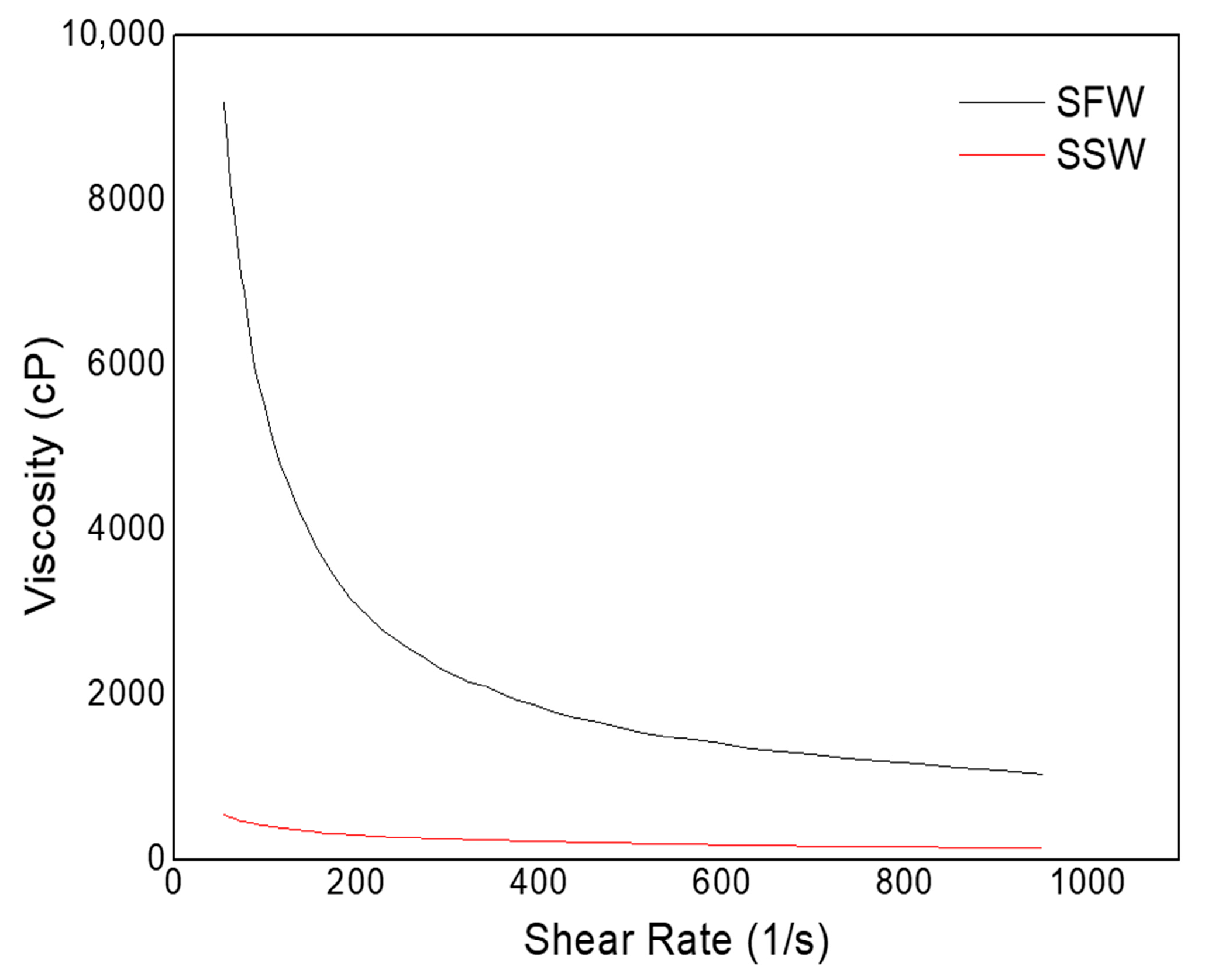
| Solutions | R2 | K (cP) | n |
|---|---|---|---|
| SFW | 0.97 | 242.23 | 0.19 |
| SSW | 0.99 | 3.10 | 0.56 |
| Exposure Time and Temperature | Mass Loss (%) | Temperature Range (°C) | Polymer Degradation During Exposure to Temperature |
|---|---|---|---|
| 70 °C/24 h | 1.55 | 221–317 | No |
| 70 °C/72 h | 1.33 | 225–321 | No |
| 110 °C/48 h | 0.80 | 232–309 | No |
| 110 °C/48 h | 0.98 | 240–303 | No |
| 110 °C/48 h | 0.74 | 251–308 | No |
| 150 °C/24 h | * | 27–125 | Yes |
| 150 °C/72 h | * | 29–133 | Yes |
| Condition of Temperature/Time | Color (mq Pt–Co/L) |
|---|---|
| Room Temperature | 127 |
| 70 °C/24 h | 126 |
| 70 °C/72 h | 128 |
| 110 °C/48 h | 153 |
| 150 °C/24 h | >500 |
| 150 °C/72 h | >500 |
| Coefficient of Determination (R2) | 97.41% |
| Fcalculated/Ftabulated | 25.02 |
| Temperature/ Exposure Time | R2 | K (cP) | n |
|---|---|---|---|
| 70 °C/24 h | 0.99 | 1.90 | 0.62 |
| 70 °C/72 h | 0.99 | 1.09 | 0.68 |
| 110 °C/48 h | 0.99 | 0.03 | 0.96 |
| 150 °C/24 h | 0.99 | 0.00 | 1.28 |
| 150 °C/72 h | 0.99 | 0.00 | 1.51 |
Disclaimer/Publisher’s Note: The statements, opinions and data contained in all publications are solely those of the individual author(s) and contributor(s) and not of MDPI and/or the editor(s). MDPI and/or the editor(s) disclaim responsibility for any injury to people or property resulting from any ideas, methods, instructions or products referred to in the content. |
© 2025 by the authors. Licensee MDPI, Basel, Switzerland. This article is an open access article distributed under the terms and conditions of the Creative Commons Attribution (CC BY) license (https://creativecommons.org/licenses/by/4.0/).
Share and Cite
Farias, M.C.d.S.; Costa, W.R.P.d.; Nóbrega, K.C.; Romualdo, V.B.; Costa, A.C.A.; Nascimento, R.C.A.d.M.; Amorim, L.V. Thermal Degradation of Carboxymethyl Cellulose (CMC) in Saline Solution for Applications in Petroleum Industry Fluids. Polymers 2025, 17, 2085. https://doi.org/10.3390/polym17152085
Farias MCdS, Costa WRPd, Nóbrega KC, Romualdo VB, Costa ACA, Nascimento RCAdM, Amorim LV. Thermal Degradation of Carboxymethyl Cellulose (CMC) in Saline Solution for Applications in Petroleum Industry Fluids. Polymers. 2025; 17(15):2085. https://doi.org/10.3390/polym17152085
Chicago/Turabian StyleFarias, Mirele Costa da Silva, Waleska Rodrigues Pontes da Costa, Karine Castro Nóbrega, Victória Bezerra Romualdo, Anna Carolina Amorim Costa, Renalle Cristina Alves de Medeiros Nascimento, and Luciana Viana Amorim. 2025. "Thermal Degradation of Carboxymethyl Cellulose (CMC) in Saline Solution for Applications in Petroleum Industry Fluids" Polymers 17, no. 15: 2085. https://doi.org/10.3390/polym17152085
APA StyleFarias, M. C. d. S., Costa, W. R. P. d., Nóbrega, K. C., Romualdo, V. B., Costa, A. C. A., Nascimento, R. C. A. d. M., & Amorim, L. V. (2025). Thermal Degradation of Carboxymethyl Cellulose (CMC) in Saline Solution for Applications in Petroleum Industry Fluids. Polymers, 17(15), 2085. https://doi.org/10.3390/polym17152085