Author Contributions
Conceptualization, A.I.P. and M.T.; methodology, A.I.P., A.D., M.T., E.-E.S., C.C., F.Z. and G.B.; software, E.-E.S., C.C., F.Z. and G.B.; validation, M.T. and A.I.P.; formal analysis, M.T.; investigation, A.I.P., A.D., M.T., E.-E.S., C.C., F.Z. and G.B.; resources, A.I.P., A.D., M.T., E.-E.S., C.C., F.Z. and G.B.; data curation, A.I.P., A.D., M.T., E.-E.S., C.C., F.Z. and G.B.; writing—original draft preparation, M.T. and A.I.P.; writing—review and editing A.I.P., A.D., M.T., E.-E.S., C.C., F.Z. and G.B.; visualization, A.I.P., A.D., M.T., E.-E.S., C.C., F.Z. and G.B.; supervision, M.T.; project administration, M.T.; funding acquisition, A.I.P., A.D., M.T., E.-E.S., C.C., F.Z. and G.B. All authors have read and agreed to the published version of the manuscript.
Figure 1.
Co-occurrence analysis of author keywords: (a) WOS search using the terms (TS = (Recycled PLA)) OR TS = (Recycled polylactic acid) AND (TS = (annealing)) OR TS = (post-processing treatment); (b) WOS search using the terms TS = (3D-printed PLA)) AND (TS = (annealing)) OR TS = (post-processing treatment) AND (TS = (machine learning)) OR TS = (optimization).
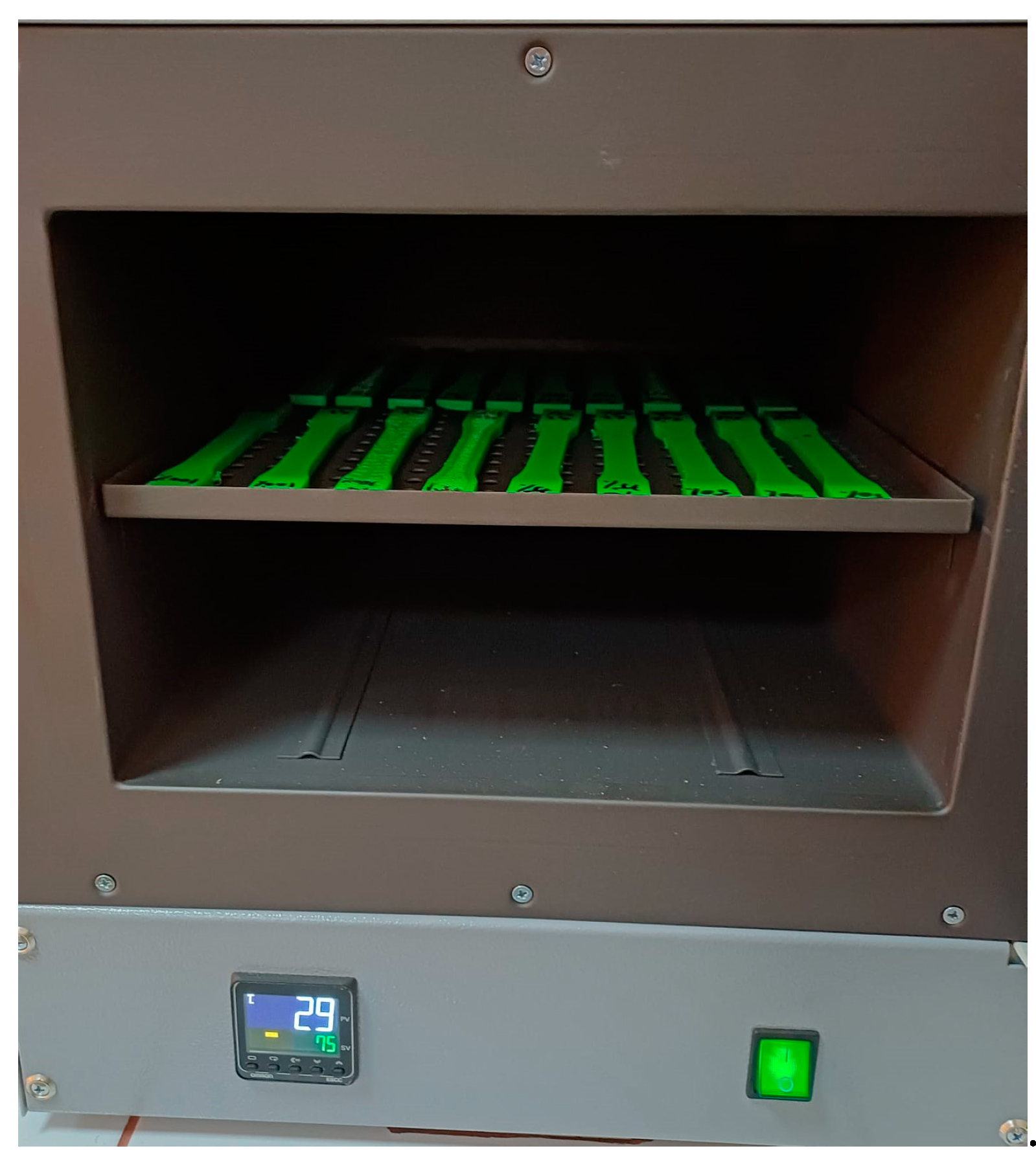
Figure 2.
Three-dimensionally printed recycled PLA samples subjected to annealing treatment.
Figure 2.
Three-dimensionally printed recycled PLA samples subjected to annealing treatment.
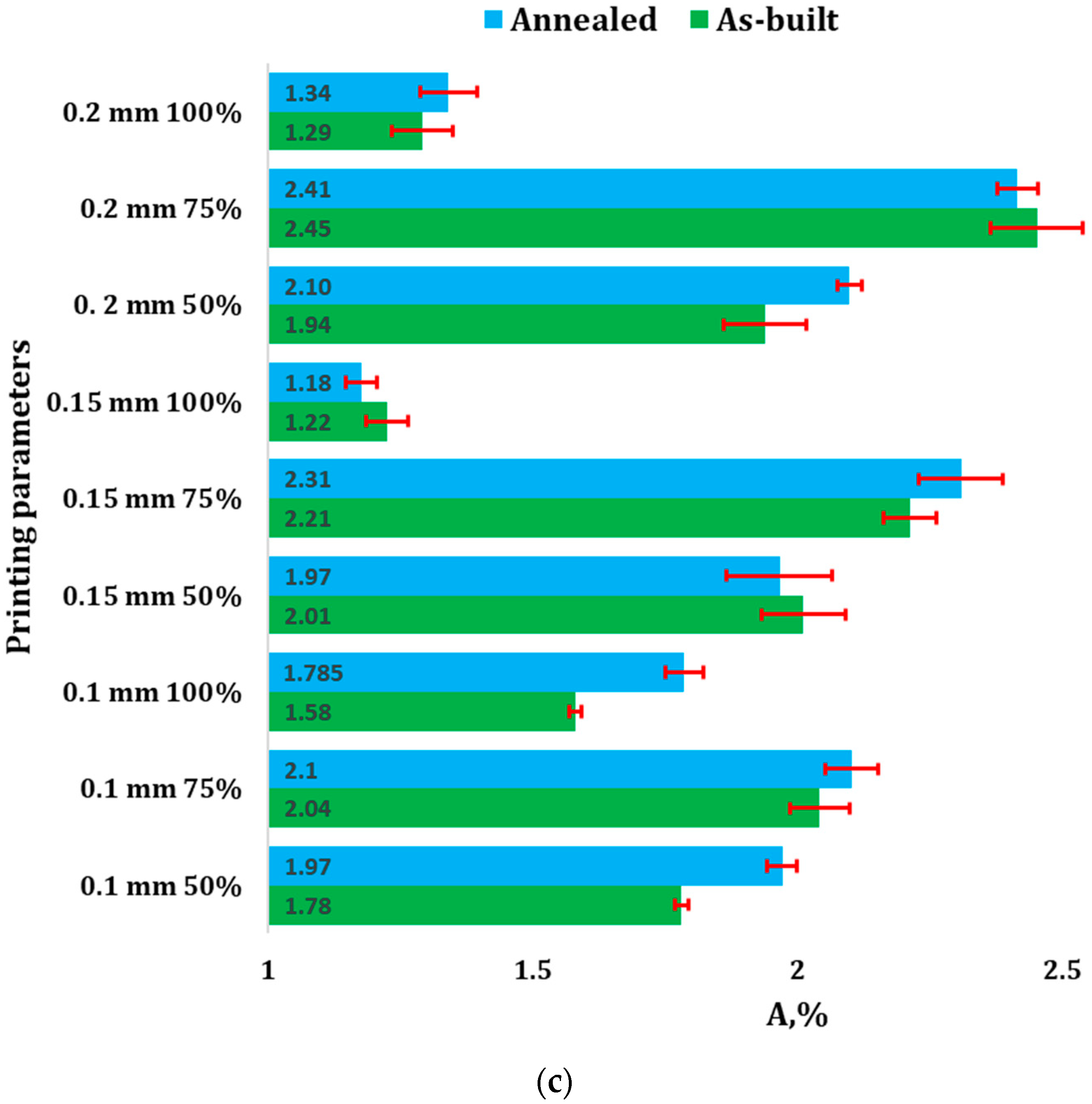
Figure 3.
Mechanical properties of 3D-printed recycled PLA samples: (a) ultimate tensile strength (UTS); (b) Young’s Modulus; (c) elongation at break (A).
Figure 3.
Mechanical properties of 3D-printed recycled PLA samples: (a) ultimate tensile strength (UTS); (b) Young’s Modulus; (c) elongation at break (A).
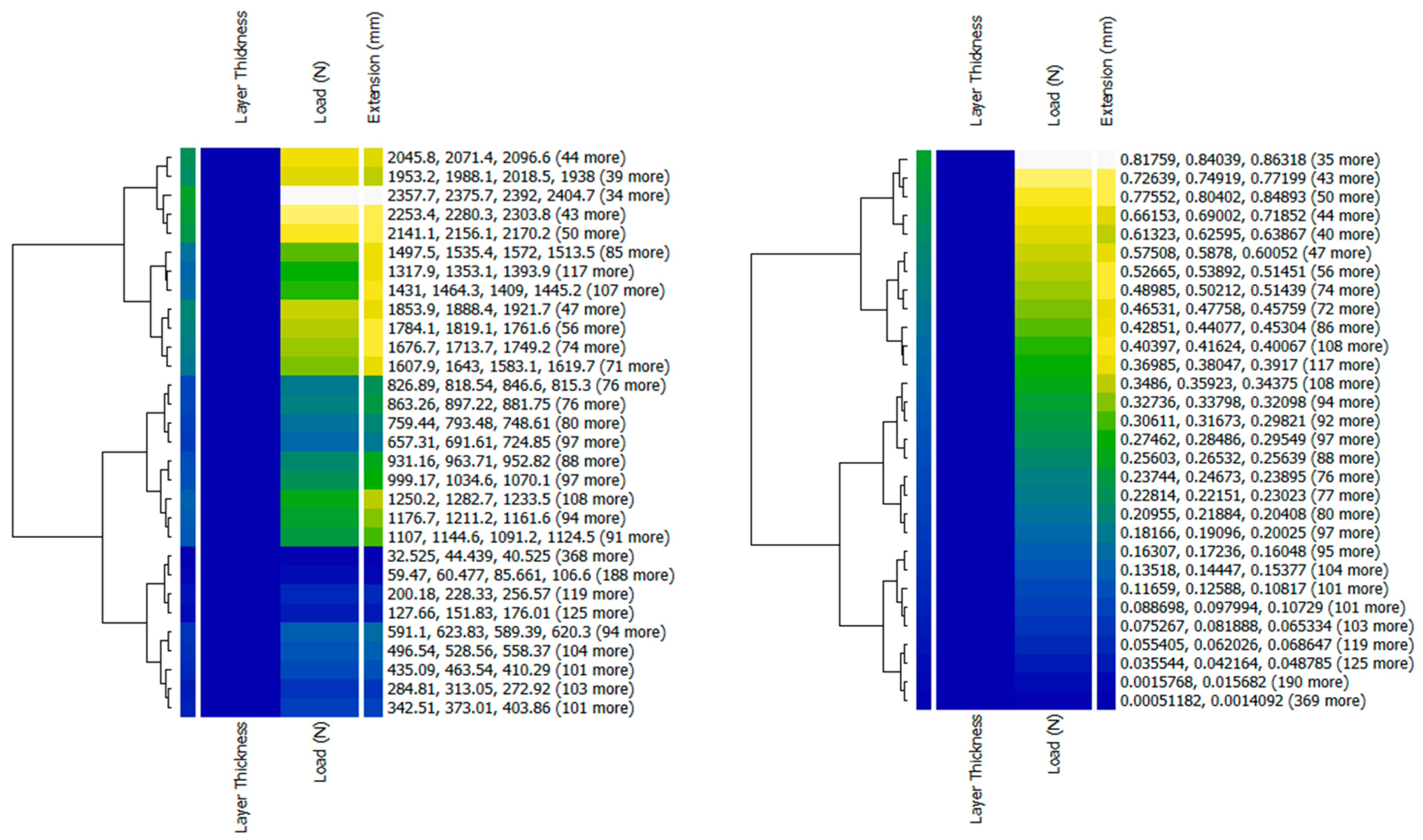
Figure 4.
The intensity of data points illustrated with heatmaps.
Figure 4.
The intensity of data points illustrated with heatmaps.
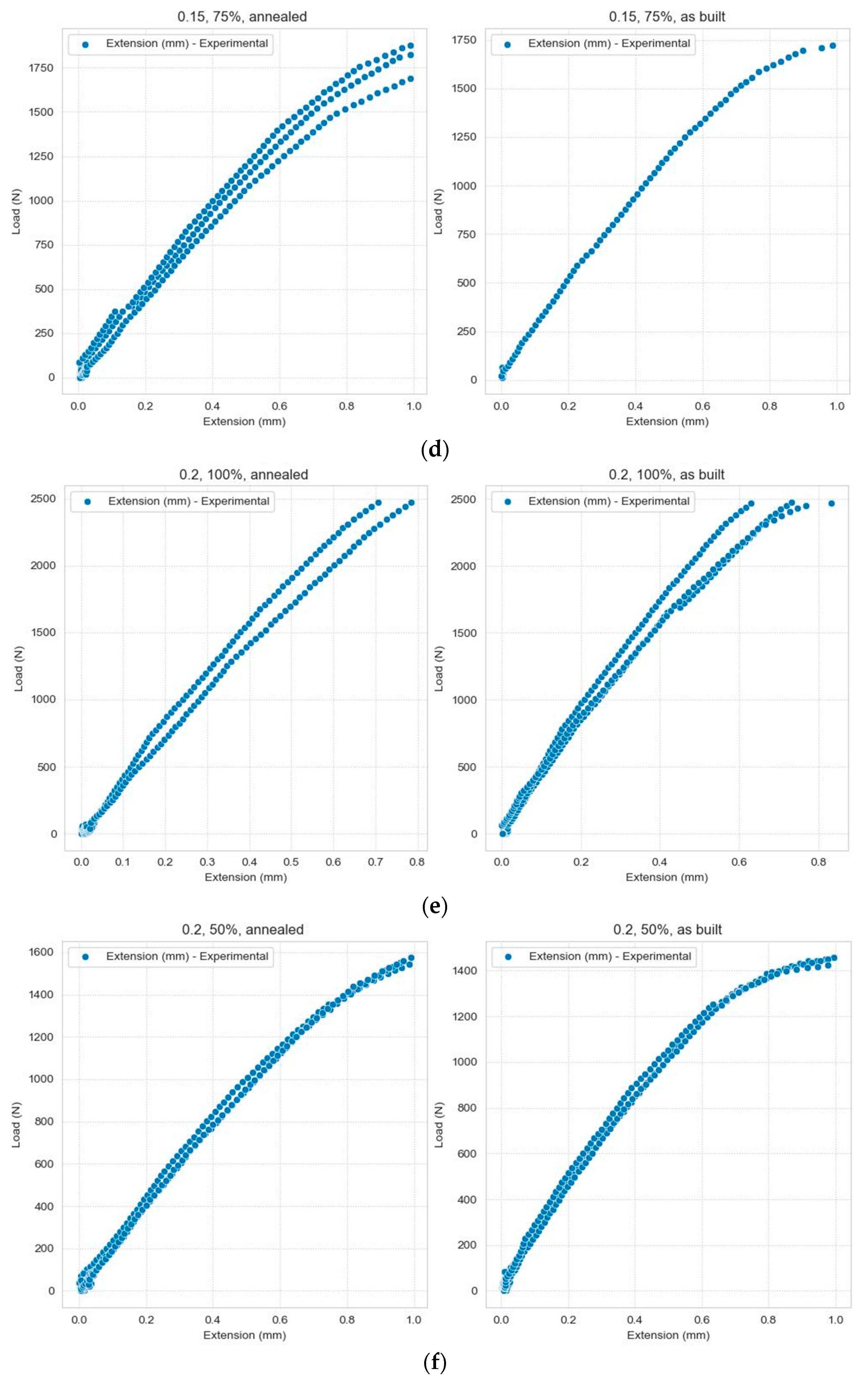
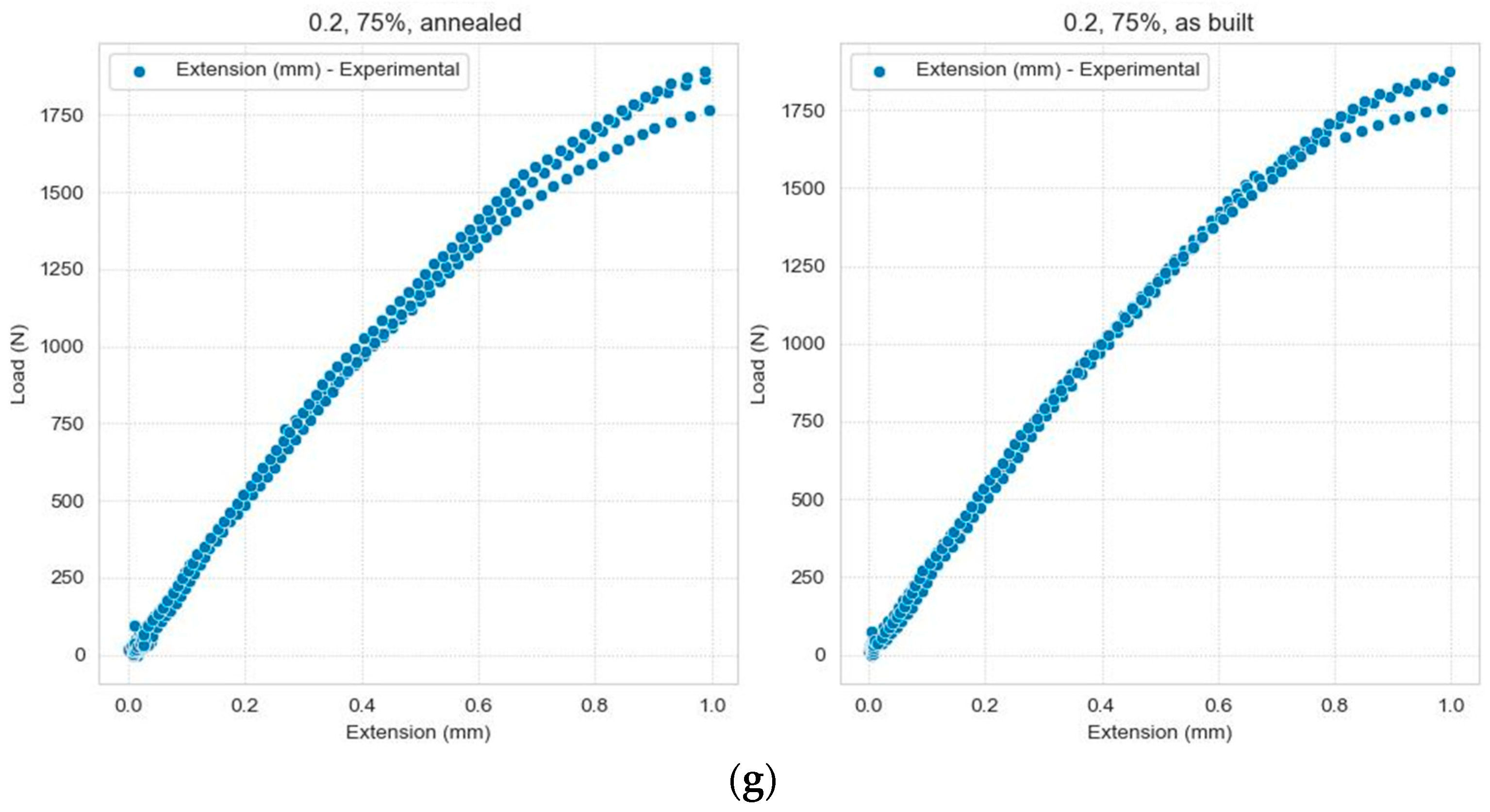
Figure 5.
Variations in the Extension depending on the Load, grouped according to the three types of categorical data: (a) Layer Thickness = 0.1 mm, Infill density = 100%; (b) Layer Thickness = 0.15 mm, Infill density = 100%; (c) Layer Thickness = 0.15 mm, Infill density = 50%; (d) Layer Thickness = 0.15 mm, Infill density = 75%; (e) Layer Thickness = 0.2 mm, Infill density = 100%; (f) Layer Thickness = 0.2 mm, Infill density = 50%; (g) Layer Thickness = 0.2 mm, Infill density = 75%.
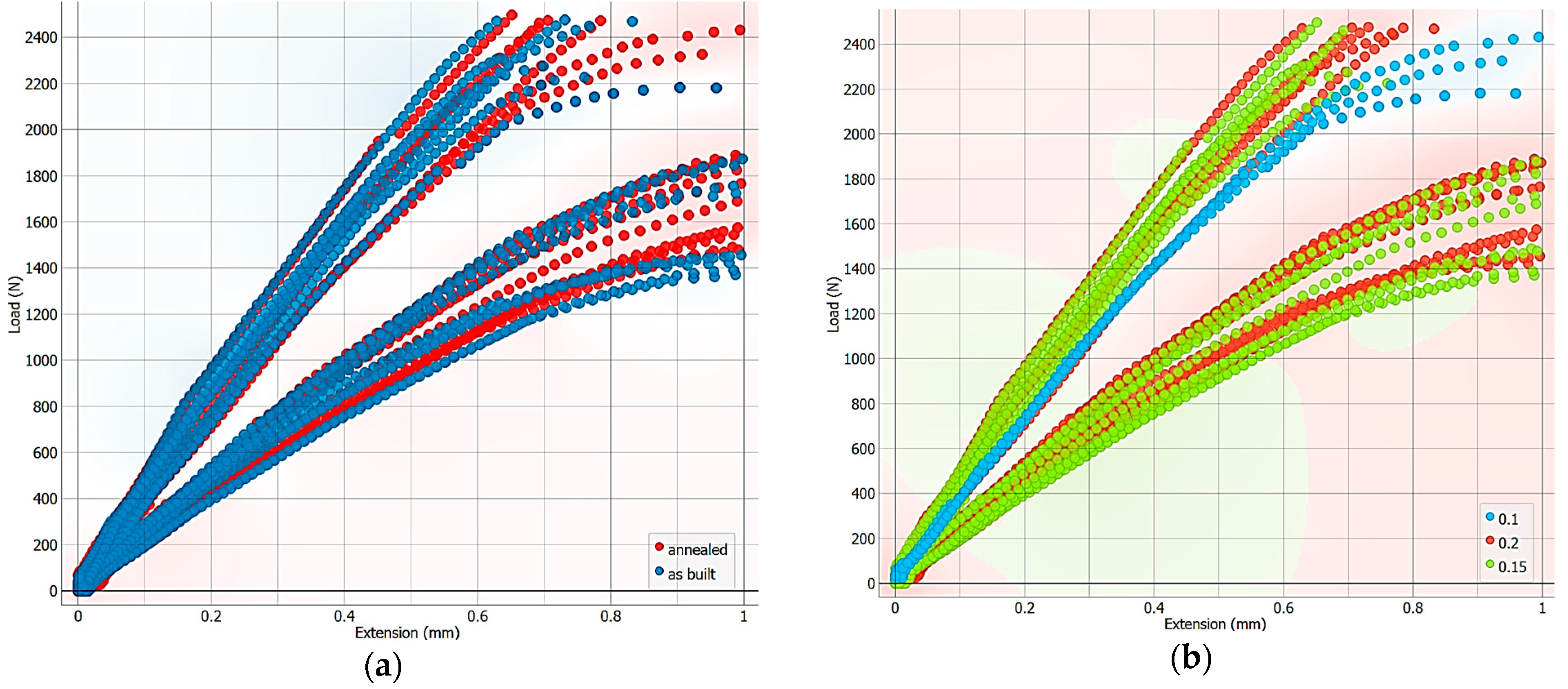
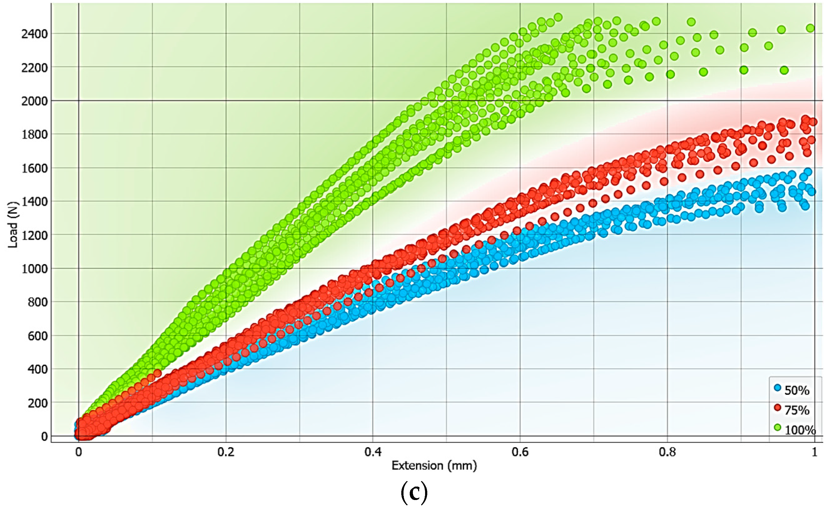
Figure 6.
The dependency between Load and Extension: (a) under different heat-treated conditions, (b) based on layer thickness (mm), and (c) based on infill density.
Figure 6.
The dependency between Load and Extension: (a) under different heat-treated conditions, (b) based on layer thickness (mm), and (c) based on infill density.
Figure 7.
Comparison between the values in the test dataset and the prediction values.
Figure 7.
Comparison between the values in the test dataset and the prediction values.
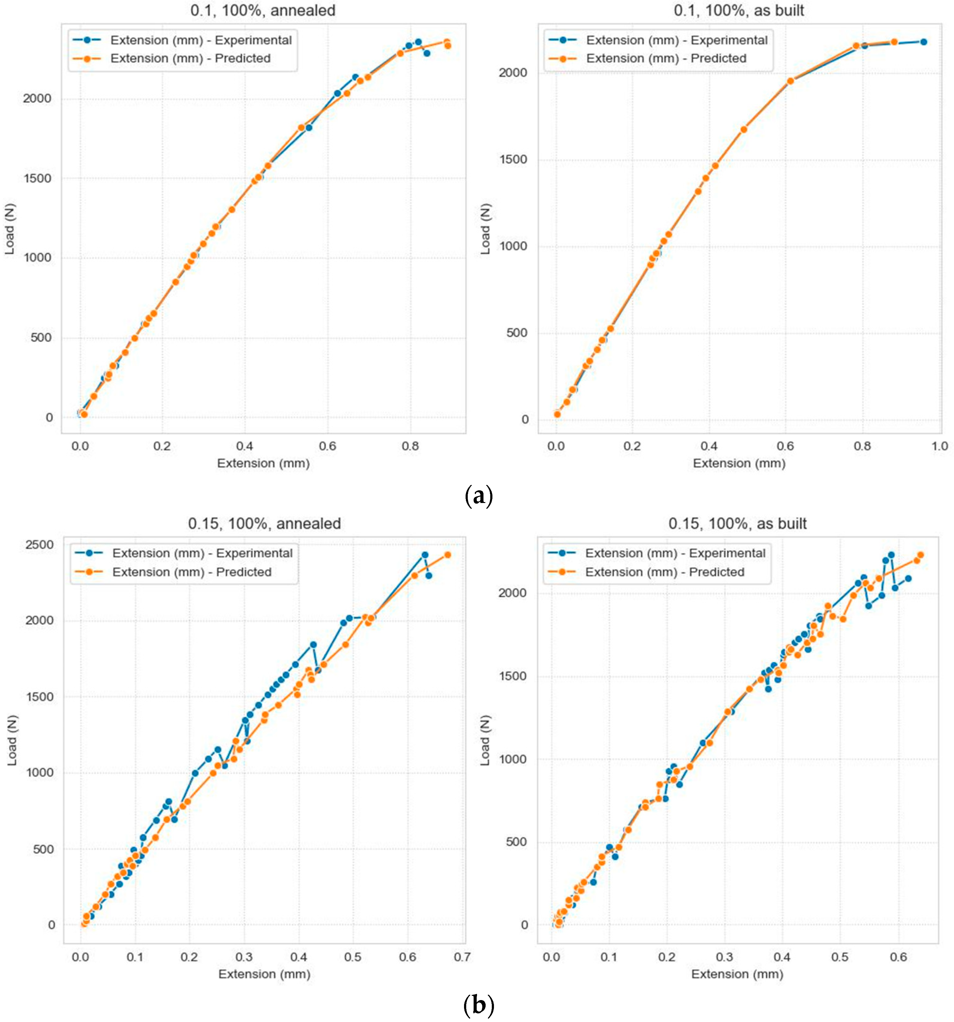
Figure 8.
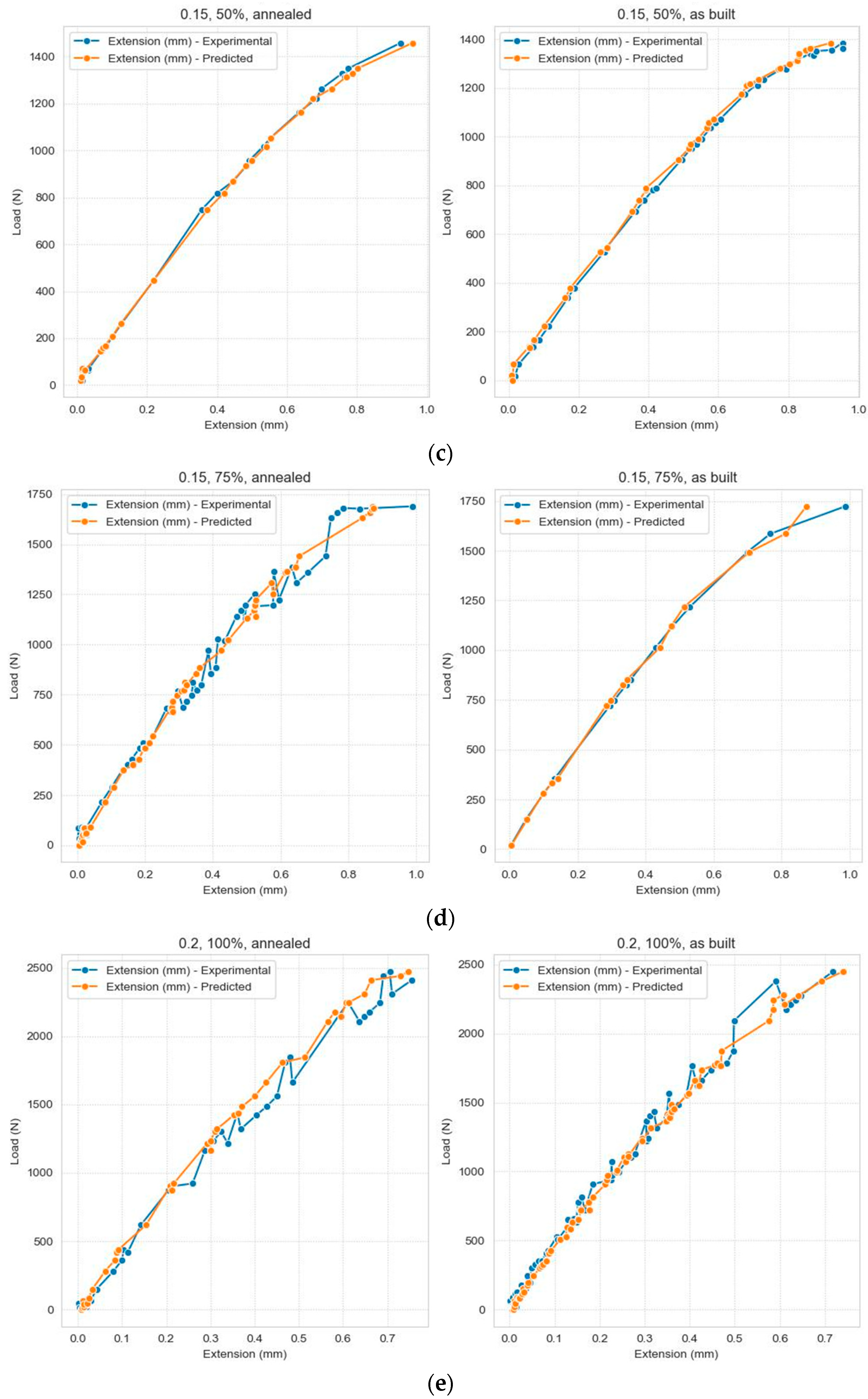
Comparison between the values in the test dataset and the predicted values, grouped according to the three categorical data: (a) Layer Thickness = 0.1 mm, Infill density = 100%; (b) Layer Thickness = 0.15 mm, Infill density = 100%; (c) Layer Thickness = 0.15 mm, Infill density = 50%; (d) Layer Thickness = 0.15 mm, Infill density = 75%; (e) Layer Thickness = 0.2 mm, Infill density = 100%; (f) Layer Thickness = 0.2 mm, Infill density = 50%; (g) Layer Thickness = 0.2 mm, Infill density = 75%.
Figure 8.
Comparison between the values in the test dataset and the predicted values, grouped according to the three categorical data: (a) Layer Thickness = 0.1 mm, Infill density = 100%; (b) Layer Thickness = 0.15 mm, Infill density = 100%; (c) Layer Thickness = 0.15 mm, Infill density = 50%; (d) Layer Thickness = 0.15 mm, Infill density = 75%; (e) Layer Thickness = 0.2 mm, Infill density = 100%; (f) Layer Thickness = 0.2 mm, Infill density = 50%; (g) Layer Thickness = 0.2 mm, Infill density = 75%.
Figure 9.
Violin plots for the prediction error distribution based on (a) layer thickness, (b) infill density, and (c) samples.
Figure 9.
Violin plots for the prediction error distribution based on (a) layer thickness, (b) infill density, and (c) samples.
Figure 10.
Comparison between the dataset and predicted values.
Figure 10.
Comparison between the dataset and predicted values.
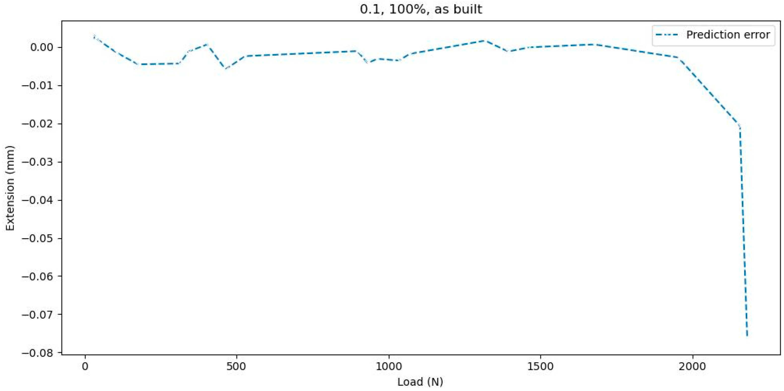
Figure 11.
Evolution of the prediction error for the test dataset (layer thickness (mm) = 0.1; infill density = ‘100%’; and samples = ‘as built’).
Figure 11.
Evolution of the prediction error for the test dataset (layer thickness (mm) = 0.1; infill density = ‘100%’; and samples = ‘as built’).
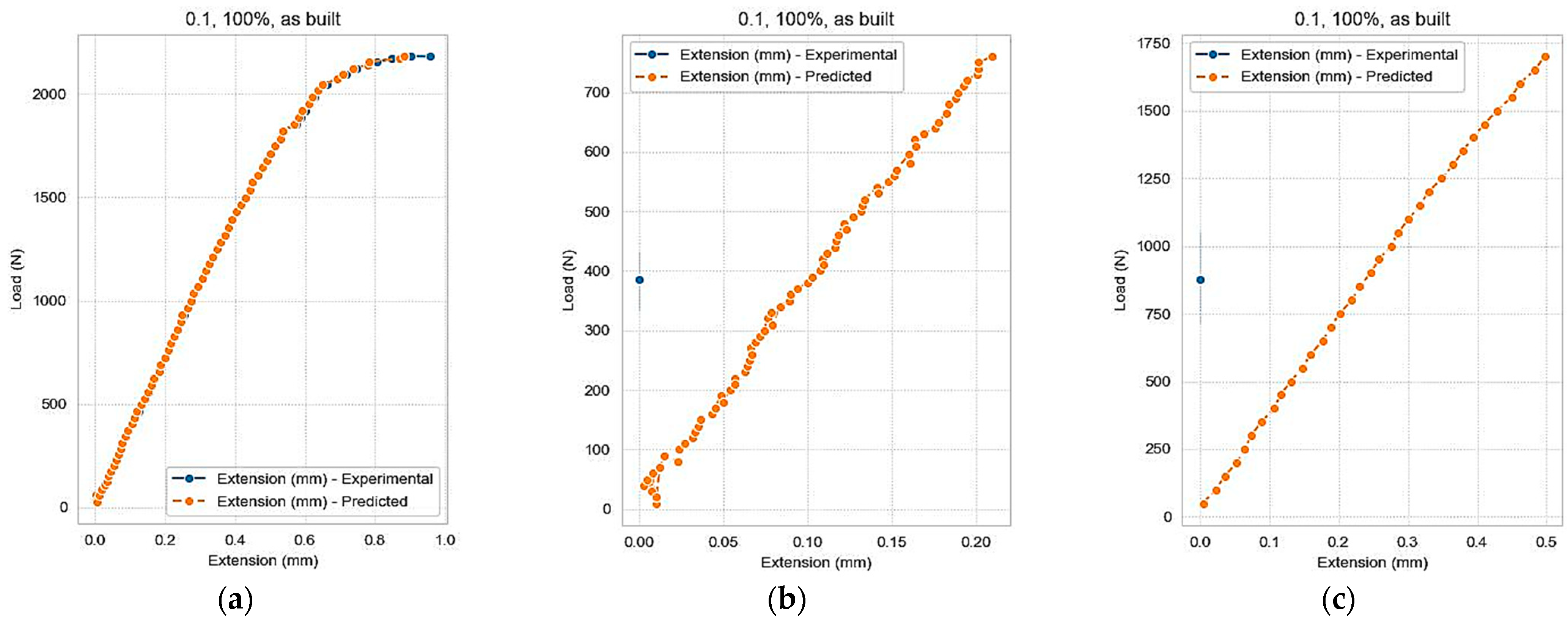
Figure 12.
Predicted Extension: (a) test 1.1, (b) test 1.2, and (c) test 1.3.
Figure 12.
Predicted Extension: (a) test 1.1, (b) test 1.2, and (c) test 1.3.
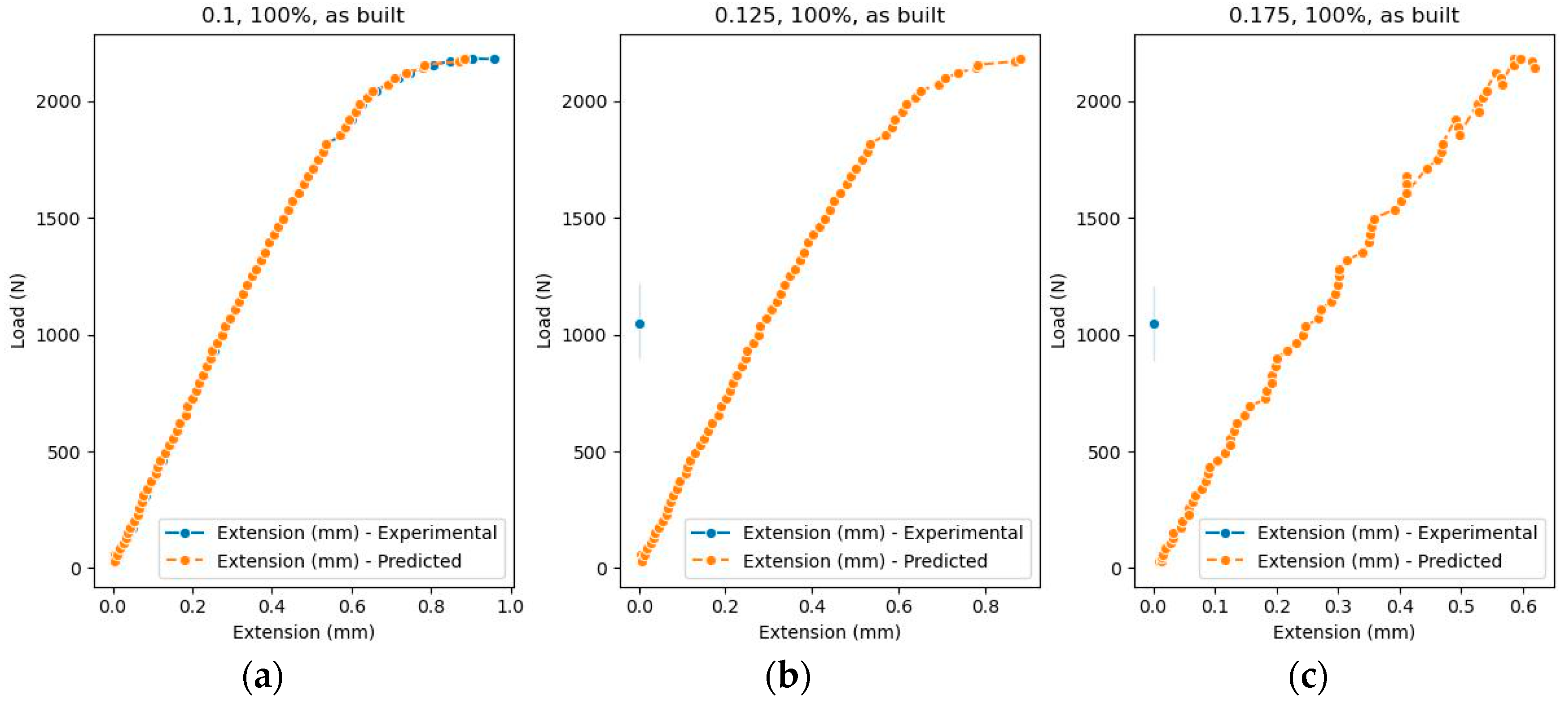
Figure 13.
Predicted Extension: (a) test 2.1, (b) test 2.2, and (c) test 2.3.
Figure 13.
Predicted Extension: (a) test 2.1, (b) test 2.2, and (c) test 2.3.
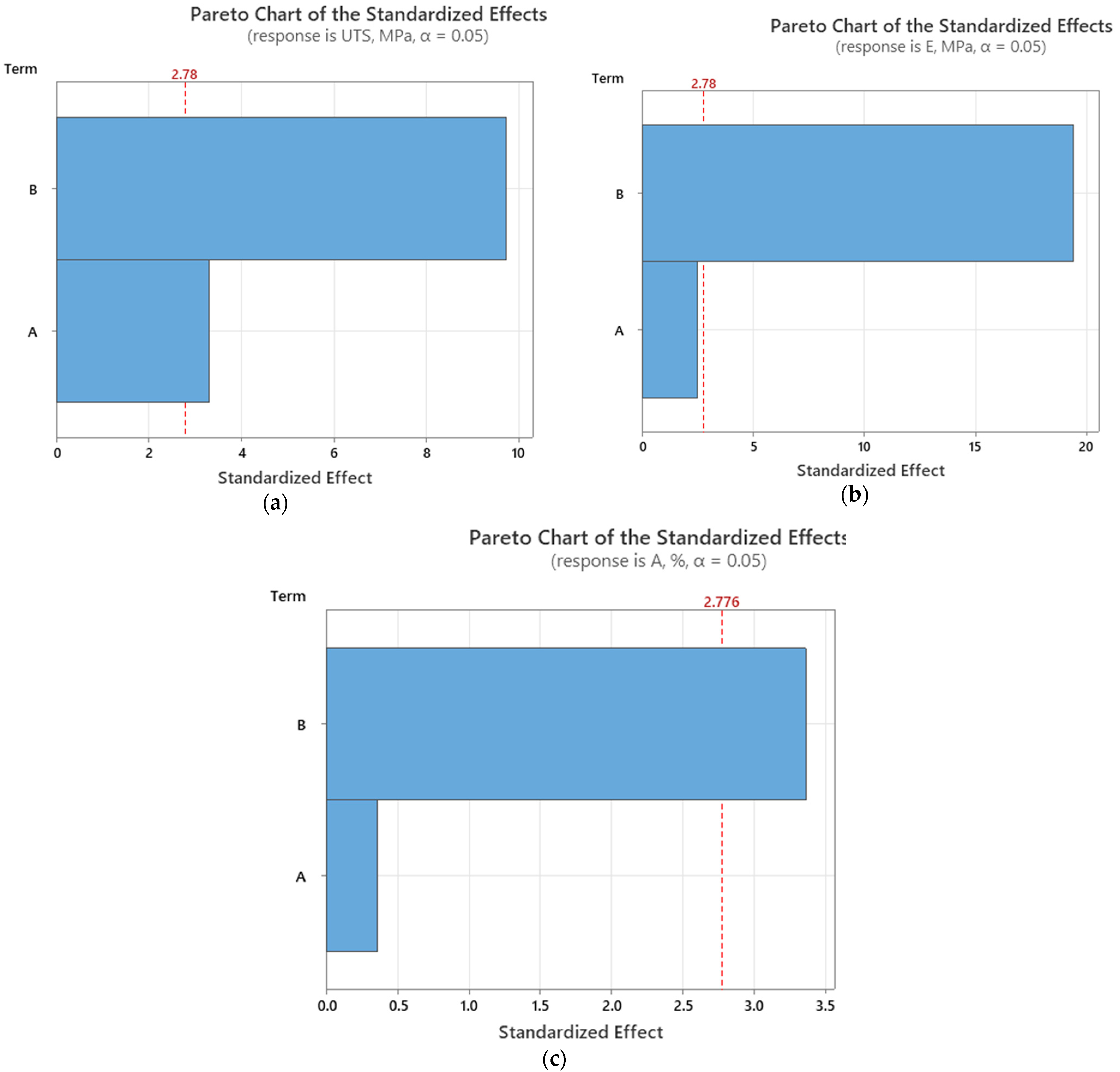
Figure 14.
Pareto charts (as-built samples) for (a) ultimate tensile strength; (b) Young’s modulus; and (c) elongation at break. (Terms: A—layer thickness; B—infill percentage).
Figure 14.
Pareto charts (as-built samples) for (a) ultimate tensile strength; (b) Young’s modulus; and (c) elongation at break. (Terms: A—layer thickness; B—infill percentage).
Figure 15.
Pareto charts (annealed samples) for (a) ultimate tensile strength; (b) Young’s modulus; and (c) elongation at break. (Terms: A—layer thickness; B—infill percentage).
Figure 15.
Pareto charts (annealed samples) for (a) ultimate tensile strength; (b) Young’s modulus; and (c) elongation at break. (Terms: A—layer thickness; B—infill percentage).
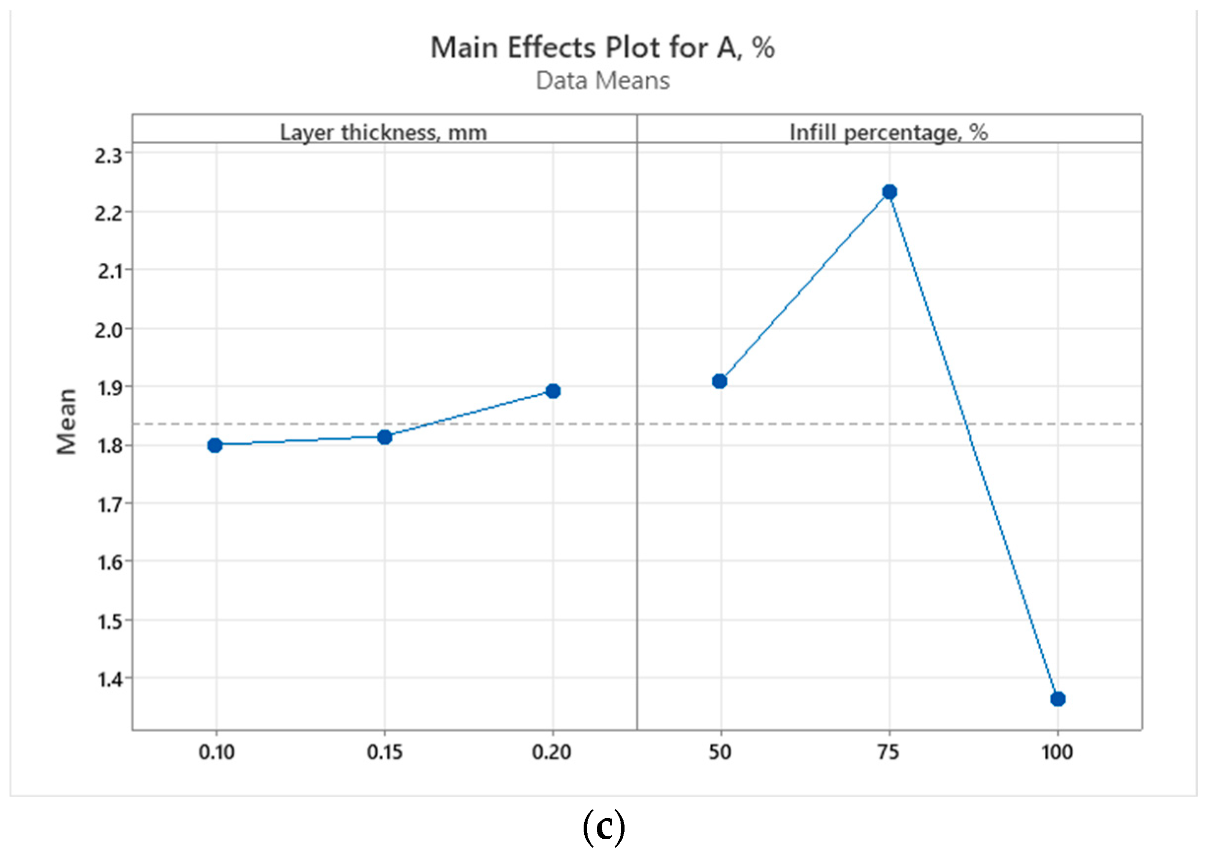
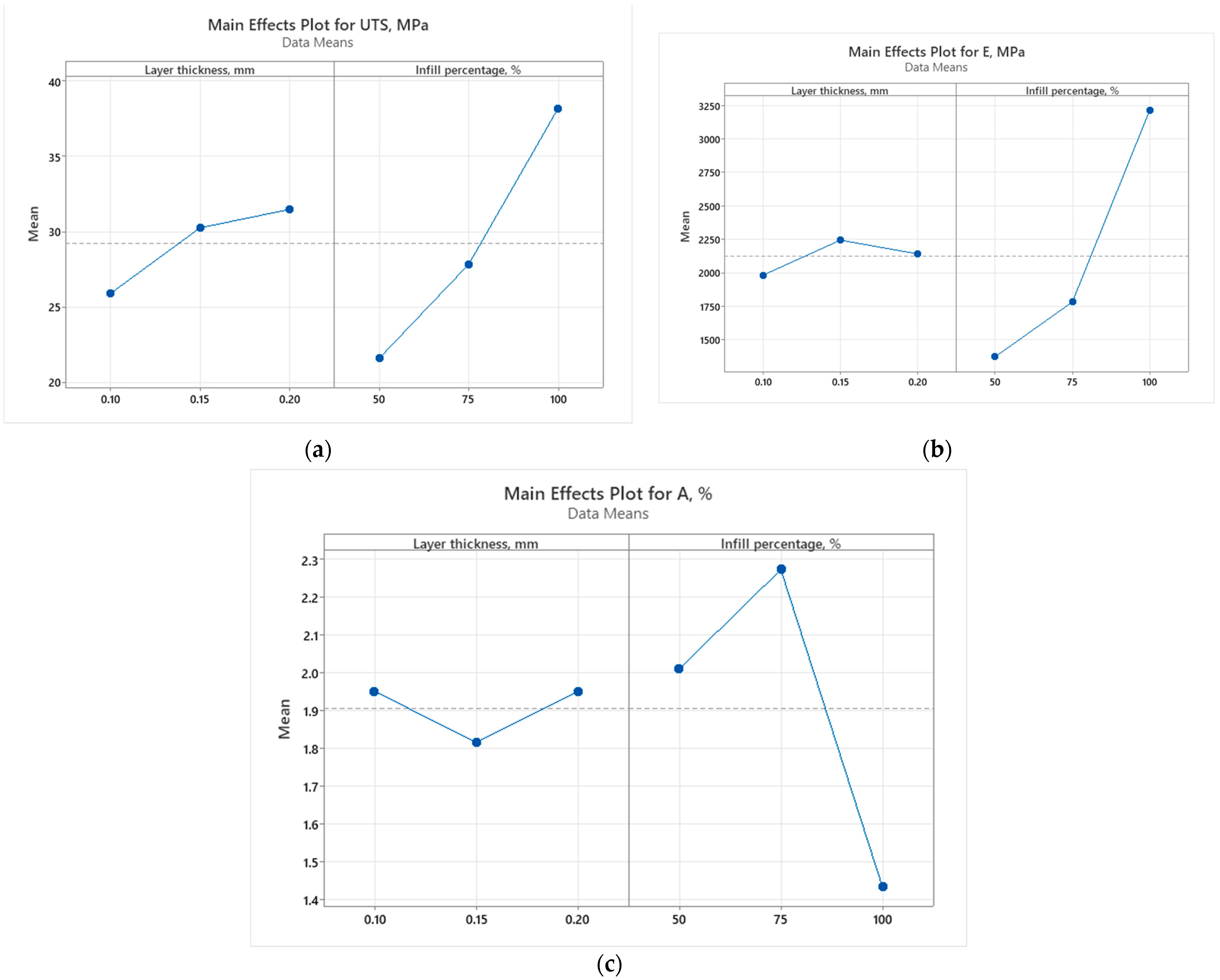
Figure 16.
Main effect plots (as-built samples) for (a) ultimate tensile strength; (b) Young’s modulus; and (c) elongation at break.
Figure 16.
Main effect plots (as-built samples) for (a) ultimate tensile strength; (b) Young’s modulus; and (c) elongation at break.
Figure 17.
Main effect plots (annealed samples) for (a) ultimate tensile strength; (b) Young’s modulus; and (c) elongation at break.
Figure 17.
Main effect plots (annealed samples) for (a) ultimate tensile strength; (b) Young’s modulus; and (c) elongation at break.
Figure 18.
Optimization plot: (a) as-built samples; (b) annealed sample.
Figure 18.
Optimization plot: (a) as-built samples; (b) annealed sample.
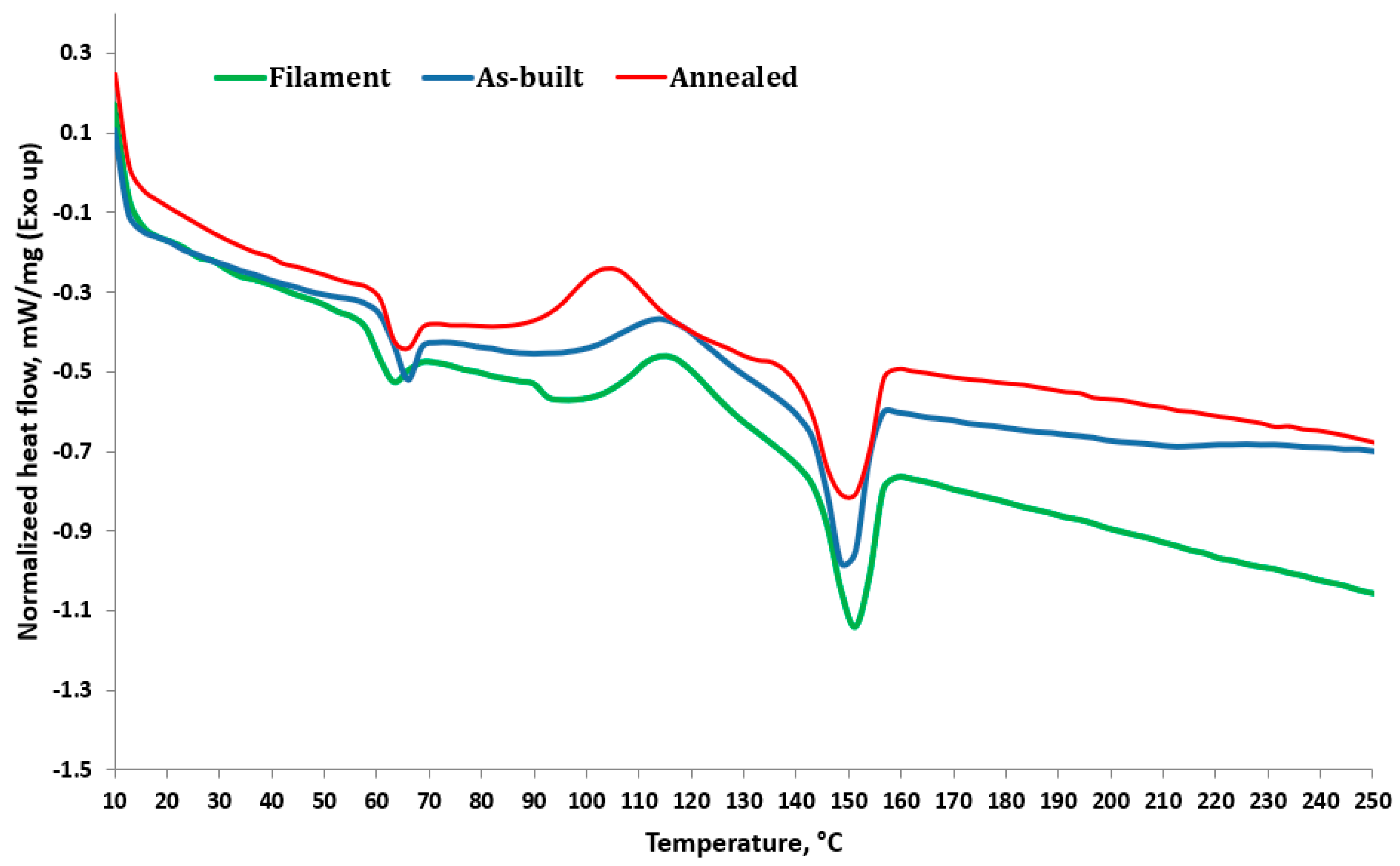
Figure 19.
DSC curves for filament, as-built, and annealed 3D-printed samples (first heating scan).
Figure 19.
DSC curves for filament, as-built, and annealed 3D-printed samples (first heating scan).
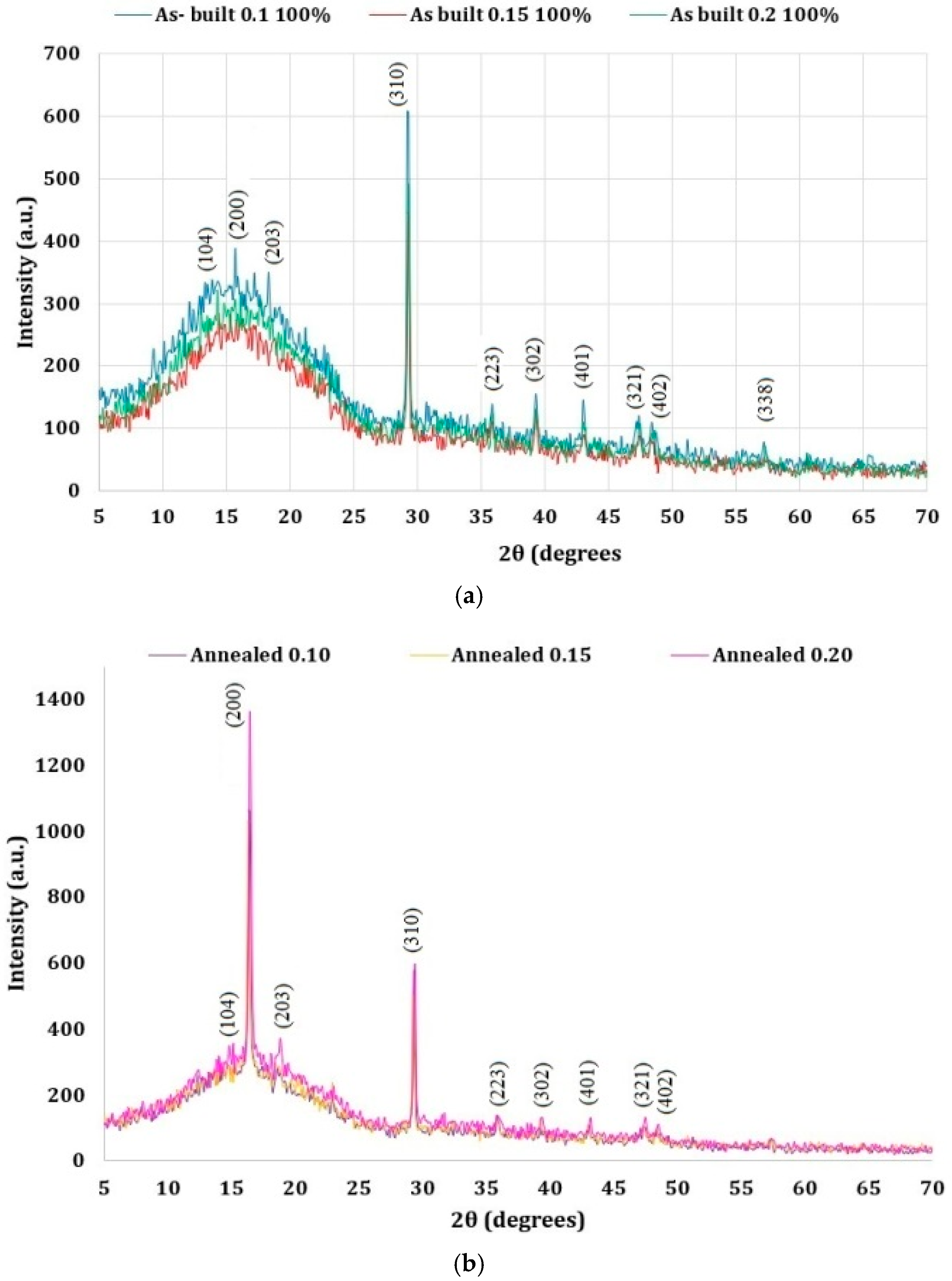
Figure 20.
XRD patterns of PLA samples: (a) as built; (b) annealed.
Figure 20.
XRD patterns of PLA samples: (a) as built; (b) annealed.
Table 1.
The printing settings.
Table 1.
The printing settings.
| Printing Options | Value |
|---|
| Shell width (mm) | 1 |
| Infill speed (mm/s) | 70 |
| Estimated print time (min) | 46 |
| Estimated filament used (g) | 10.60 |
| Extruder temperature (°C) | 210 |
| Bed temperature (°C) | 60 |
| Platform addition | Raft only |
Table 2.
Parameters and corresponding levels utilized in the DOE analysis.
Table 2.
Parameters and corresponding levels utilized in the DOE analysis.
| Parameter | Level |
|---|
| 1 | 2 | 3 |
|---|
| Layer thickness, mm | 0.10 | 0.15 | 0.20 |
| Infill percentage, % | 50 | 75 | 100 |
Table 3.
Types of data used for dataset.
Table 3.
Types of data used for dataset.
| Name | Type | Role | Values |
|---|
| Layer Thickness | Categorical | Feature | 0.1, 0.15, 0.2 |
| Infill density | Categorical | Feature | 50%, 75%, 100% |
| Samples | Categorical | Feature | Annealed, as built |
| Load | Numeric | Feature | |
| Extension | Numeric | Target | |
Table 4.
Statistical representations of the dataset.
Table 4.
Statistical representations of the dataset.
| Statistics | Layer Thickness | Load | Extension |
|---|
| count | 2946 | 2946 | 2946 |
| mean | 0.169756 | 848.5495 | 0.318202 |
| std | 0.033804 | 672.5881 | 0.269695 |
| min | 0.1 | 0 | 0 |
| 25% | 0.15 | 214 | 0.068647 |
| 50% | 0.2 | 768.94 | 0.26532 |
| 75% | 0.2 | 1357.6 | 0.517402 |
| max | 0.2 | 2496.7 | 0.99793 |
Table 5.
Key metrics used to evaluate the performance of ML algorithms.
Table 5.
Key metrics used to evaluate the performance of ML algorithms.
| Model | MSE | RMSE | MAE | MdAPE | R2 |
|---|
| Random Forest | 0.001 | 0.027 | 0.018 | 6.059579664 | 0.990 |
| Gradient Boosting | 0.001 | 0.028 | 0.019 | 6.698080301 | 0.989 |
| Tree | 0.001 | 0.030 | 0.020 | 6.977544282 | 0.988 |
| AdaBoost | 0.001 | 0.031 | 0.020 | 6.950282399 | 0.987 |
| Neural Network | 0.001 | 0.032 | 0.021 | 6.224877491 | 0.986 |
| Linear Regression | 0.008 | 0.090 | 0.073 | 21.99528675 | 0.889 |
| SVM Learner | 0.012 | 0.108 | 0.085 | 17.17770959 | 0.841 |
| kNN | 0.015 | 0.124 | 0.082 | 26.72113087 | 0.788 |
Table 6.
First and last 5 values for Load and predicted Extension for the 3 tests.
Table 6.
First and last 5 values for Load and predicted Extension for the 3 tests.
| Prediction Test 1.1 | Prediction Test 1.2 | Prediction Test 1.3 |
|---|
| Load (N) | Extension (mm)—Predicted | Load (N) | Extension (mm)—Predicted | Load (N) | Extension (mm)—Predicted |
|---|
| 32.525 | 0.0035286 | 10 | 0.0098069 | 50 | 0.00488235 |
| 44.439 | 0.00324737 | 20 | 0.0101538 | 100 | 0.023429 |
| 59.47 | 0.00423718 | 30 | 0.00729629 | 150 | 0.0363373 |
| 40.525 | 0.00278179 | 40 | 0.00278179 | 200 | 0.0537019 |
| 31.655 | 0.00434033 | 50 | 0.00488235 | 250 | 0.0653139 |
| … |
| 2141.1 | 0.779581 | 720 | 0.194466 | 1500 | 0.428727 |
| 2156.1 | 0.783324 | 730 | 0.200634 | 1550 | 0.449607 |
| 2170.2 | 0.870527 | 740 | 0.201108 | 1600 | 0.461231 |
| 2182.2 | 0.882195 | 750 | 0.201739 | 1650 | 0.482956 |
| 2180.4 | 0.882195 | 760 | 0.209748 | 1700 | 0.497015 |
Table 7.
Optimization goals for mechanical properties of as-built samples.
Table 7.
Optimization goals for mechanical properties of as-built samples.
| Response | Goal | Lower | Target | Upper | Weight | Importance |
|---|
| A, % | Maximum | 1.18 | 2.41 | | 0.33 | 1 |
| E, MPa | Maximum | 1201.50 | 3441.50 | | 0.33 | 1 |
| UTS, MPa | Maximum | 16.36 | 39.42 | | 0.33 | 1 |
Table 8.
Optimization goals for mechanical properties of annealed samples.
Table 8.
Optimization goals for mechanical properties of annealed samples.
| Response | Goal | Lower | Target | Upper | Weight | Importance |
|---|
| A, % | Maximum | 1.22 | 2.45 | | 0.33 | 1 |
| E, MPa | Maximum | 1163.50 | 3329.67 | | 0.33 | 1 |
| UTS, MPa | Maximum | 16.79 | 37.21 | | 0.33 | 1 |
Table 9.
Composite desirability and ranks.
Table 9.
Composite desirability and ranks.
| | | As Built | Annealed |
|---|
| Layer Thickness, mm | Infill Percentage, % | Composite Desirability | Rank | Composite Desirability | Rank |
|---|
| 0.10 | 50 | 0.385318 | 9 | 0.458268 | 9 |
| 0.10 | 75 | 0.740012 | 5 | 0.739367 | 6 |
| 0.10 | 100 | 0.735175 | 6 | 0.819881 | 2 |
| 0.15 | 50 | 0.580915 | 8 | 0.655372 | 7 |
| 0.15 | 75 | 0.792769 | 3 | 0.804551 | 4 |
| 0.15 | 100 | 0.766233 | 4 | 0.797615 | 5 |
| 0.20 | 50 | 0.620928 | 7 | 0.648887 | 8 |
| 0.20 | 75 | 0.817232 | 1 * | 0.809841 | 3 |
| 0.20 | 100 | 0.817221 | 2 | 0.847086 | 1 * |
Table 10.
Thermal characteristics of the analyzed samples.
Table 10.
Thermal characteristics of the analyzed samples.
| Sample Type | Mass, mg | Tg, °C | Tc, °C | Tm, °C | XC, % |
|---|
| Filament | 3.43 | 63.30 ± 0.12 | 114.00 ± 0.27 | 151.30 ± 0.22 | - |
| As built | 3.90 | 65.60 ± 0.14 | 113.95 ± 0.23 | 149.67 ± 0.17 | 42.4 |
| Annealed | 3.78 | 64.78 ± 0.21 | 104.63 ± 0.15 | 149.87 ± 0.19 | 43.6 |
Table 11.
Degree of crystallinity for the investigated 3D-printed PLA samples.
Table 11.
Degree of crystallinity for the investigated 3D-printed PLA samples.
| Layer Thickness | XRD XC (%) |
|---|
| PLA As Built | PLA Annealed |
|---|
| 0.10 | 35.77 | 43.09 |
| 0.15 | 32.44 | 43.45 |
| 0.20 | 34.55 | 45.86 |


 ,
, 


