
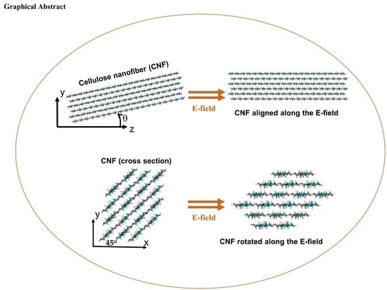
Molecular Dynamics Study of Cellulose Nanofiber Alignment under an Electric Field


Abstract
:
1. Introduction
2. Methods
3. Results and Discussion
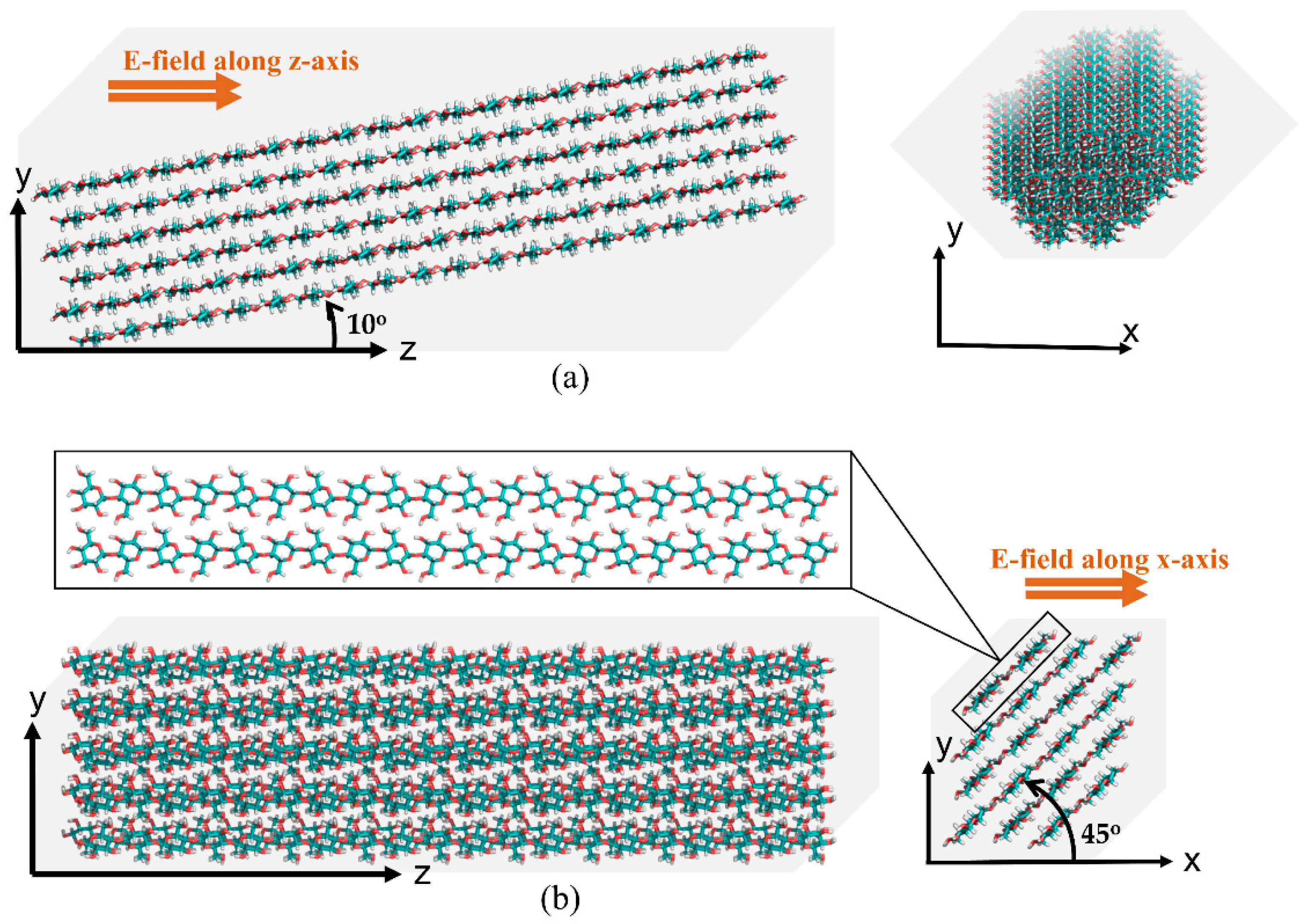
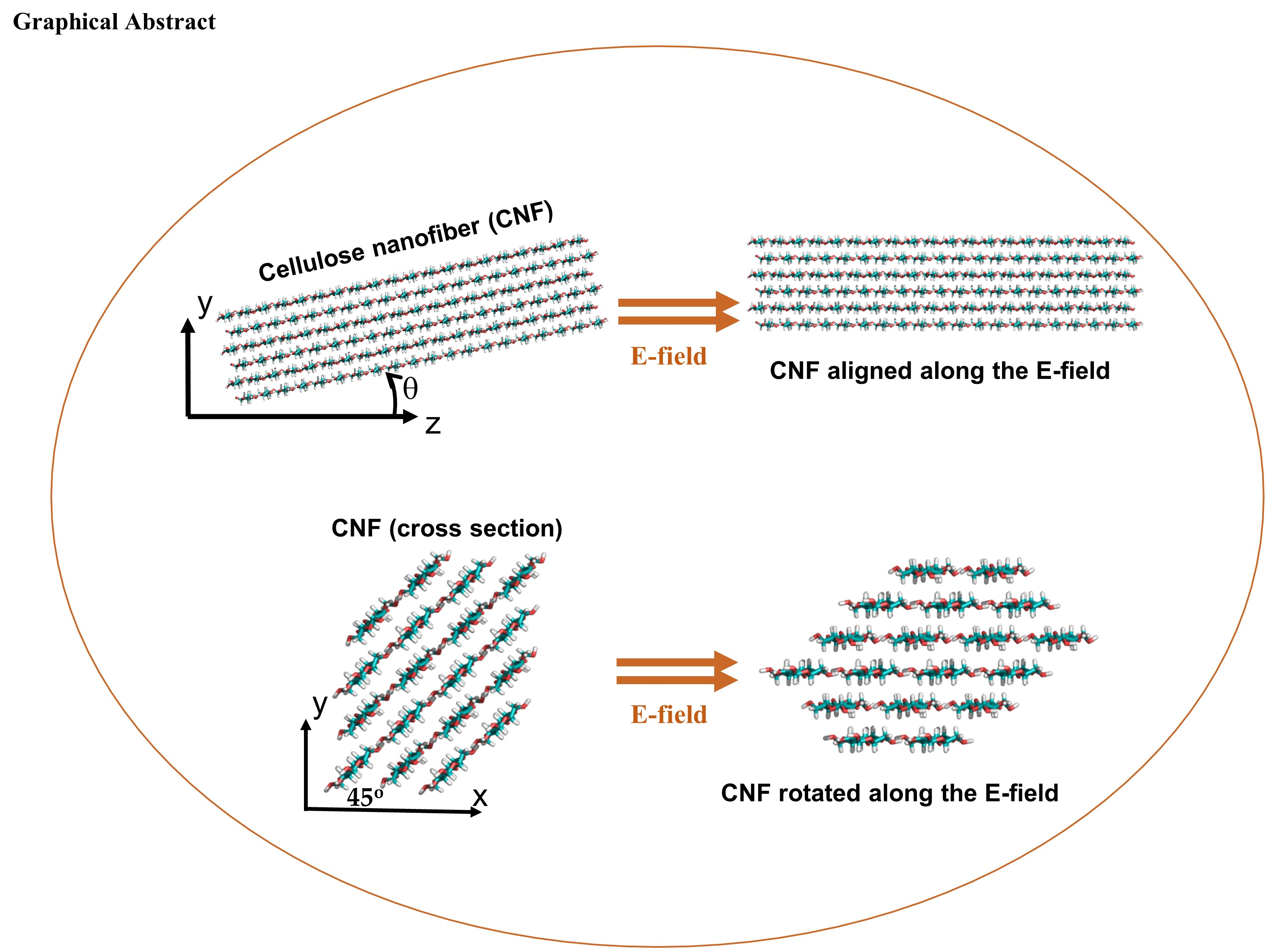
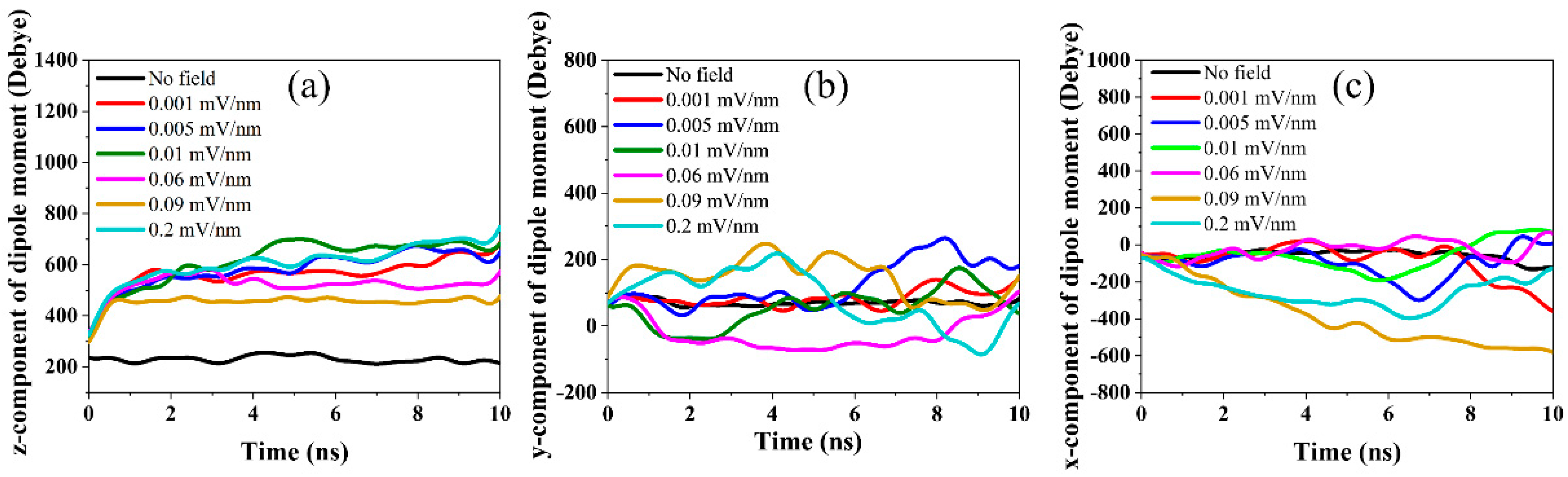
3.1. CASE 1: Electric Field along the Z-Axis
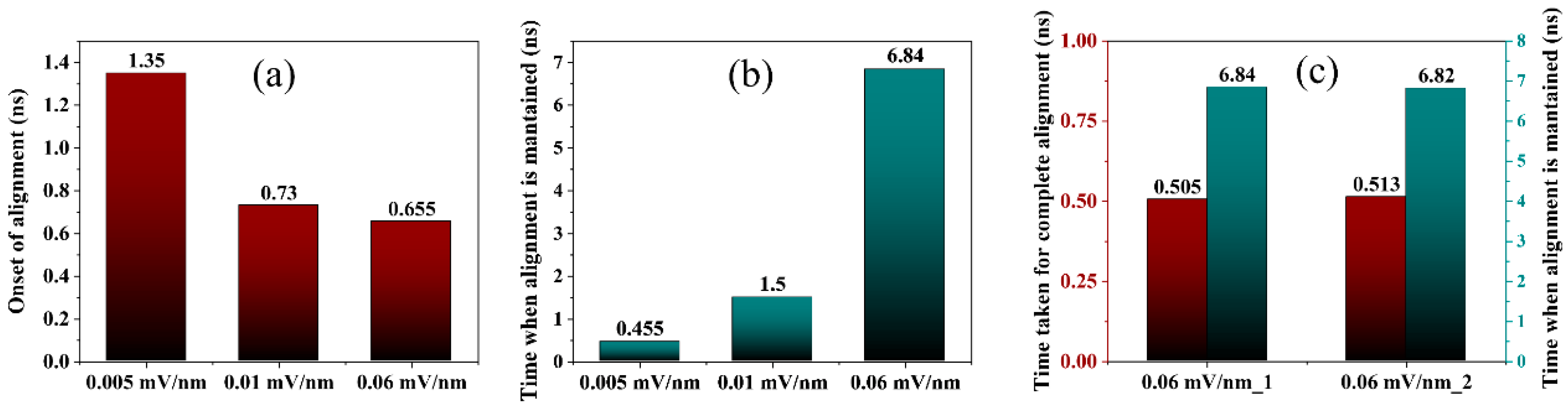
3.1.1. Electric Field-Induced Alignment of Cellulose Structure
3.1.2. Dipole Moment
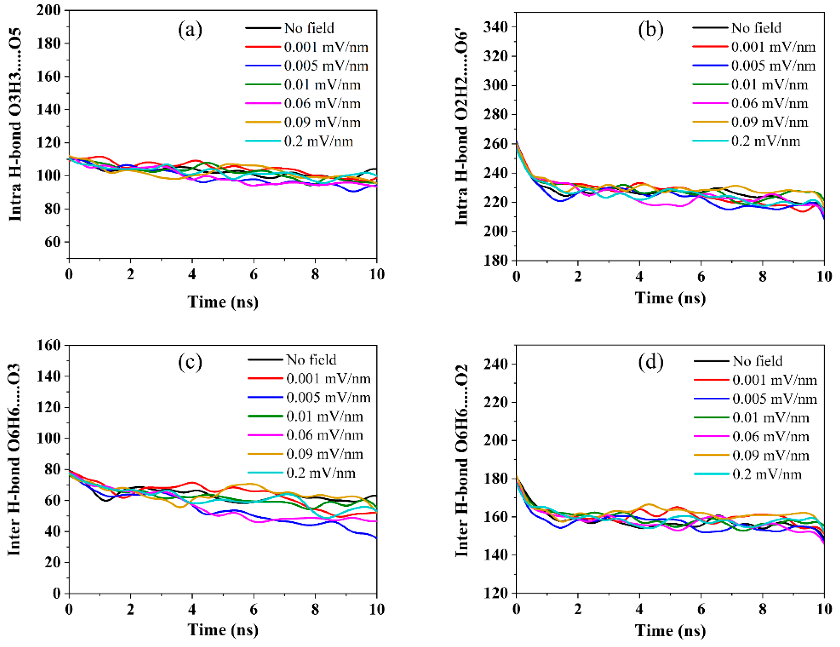
3.1.3. Effect of Electric Field on the Cellulose Structure
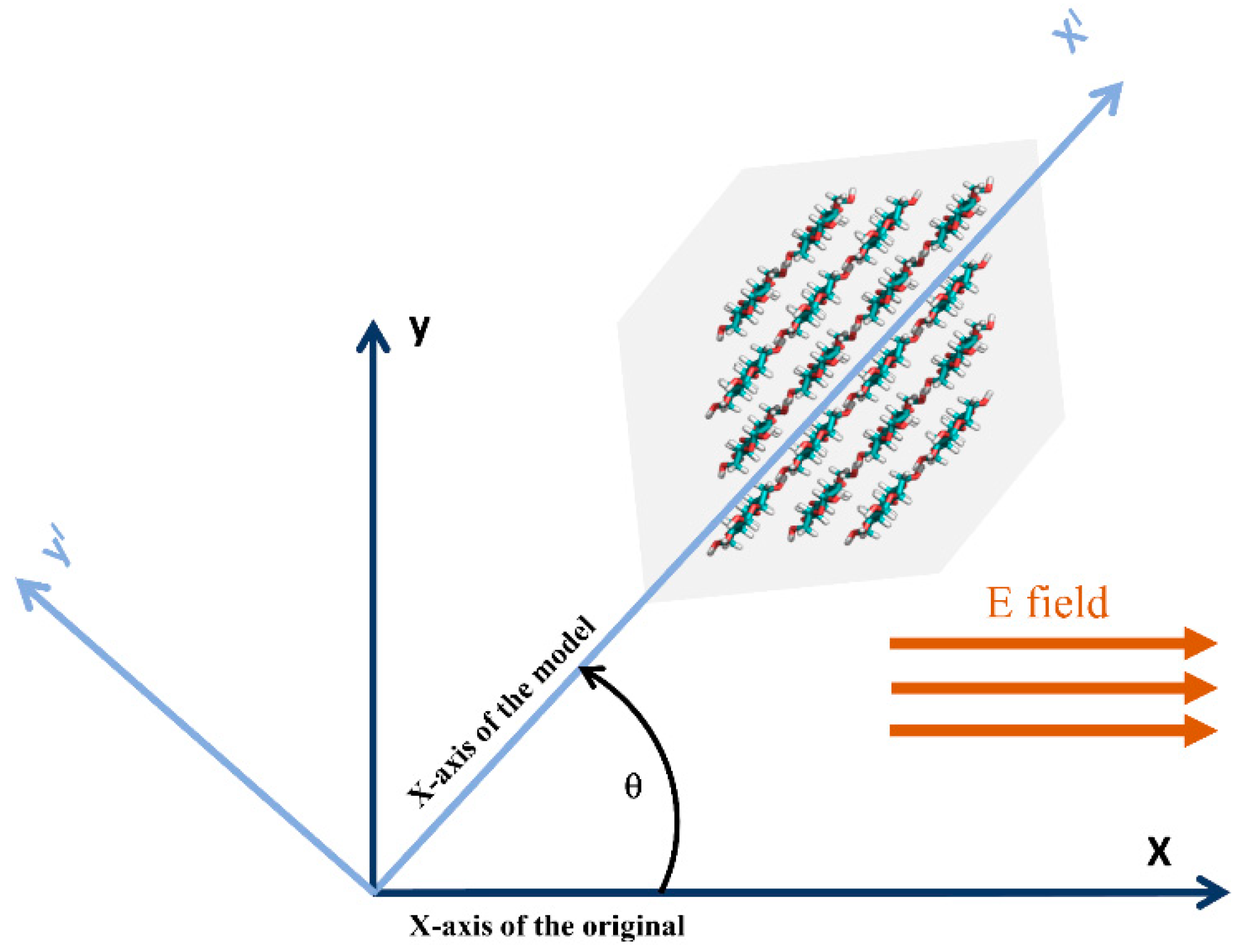
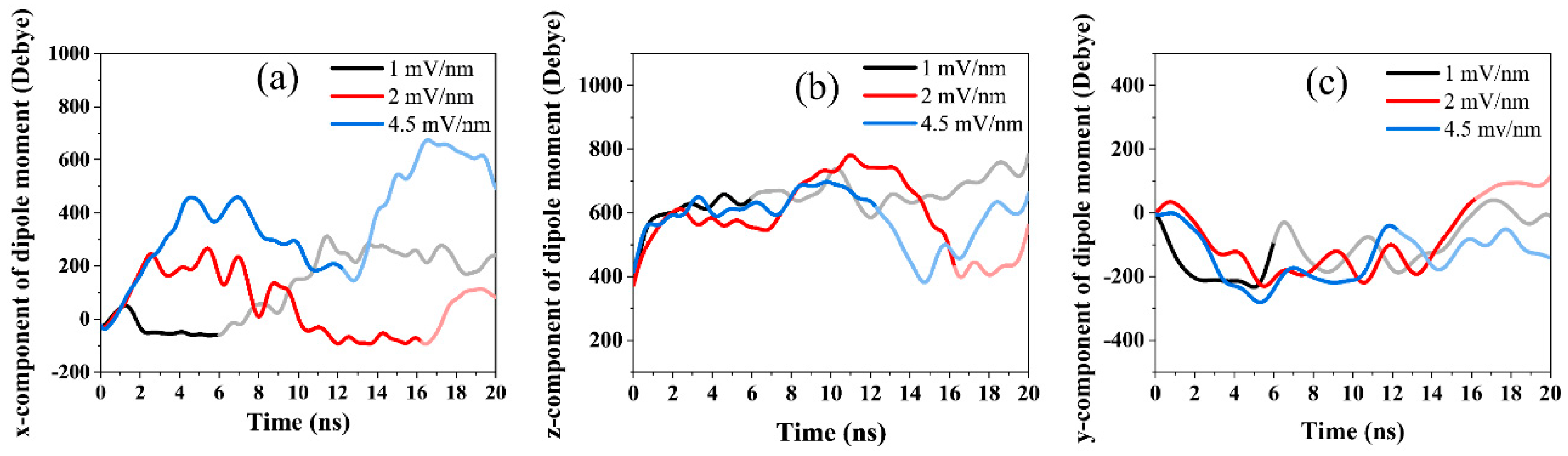
3.2. CASE 2: Electric Field along the X-Axis
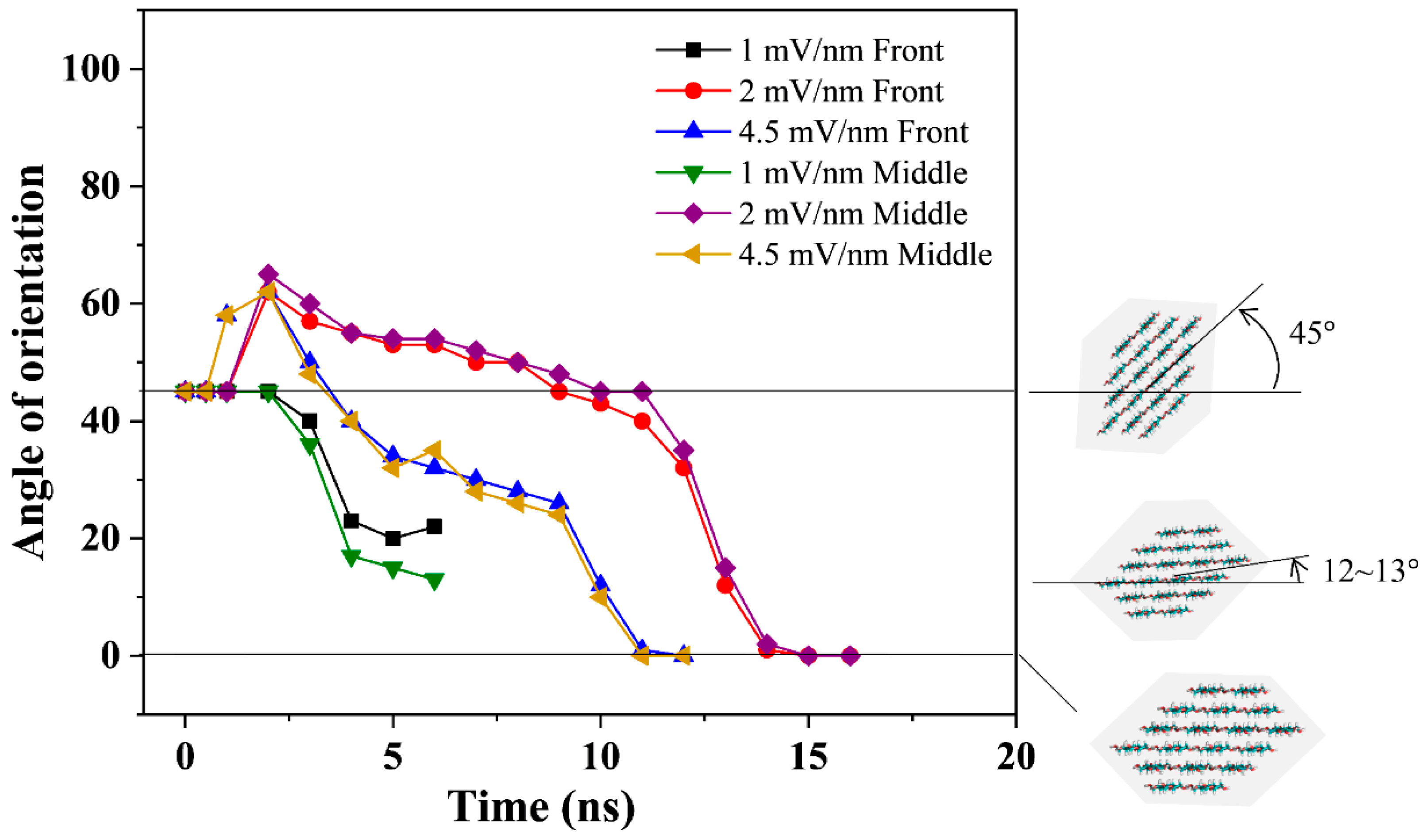
3.2.1. Alignment Effect of Electric Field on Cellulose
3.2.2. Dipole Moment
3.2.3. Stability of Cellulose Structure
4. Conclusions
Supplementary Materials
Author Contributions
Funding
Conflicts of Interest
References
- Comprehensive Cellulose Chemistry. Volume 1. Fundamentals and Analytical Methods By D. Klemm, B. Philipp, T. Heinze, U. Heinze, and W. Wagenknecht. Wiley: Weinheim, Germany. 1998. 260 pp. $236.25. ISBN 3-527-29413-9. J. Am. Chem. Soc. 1999, 121, 8677. [Google Scholar] [CrossRef]
- Klemm, D.; Philipp, B.; Heinze, T.; Heinze, U.; Wagenknecht, W. Comprehensive Cellulose Chemistry; Wiley: Hoboken, NJ, USA, 1998; ISBN 9783527294893. [Google Scholar]
- Dias, O.A.T.; Konar, S.; Leão, A.L.; Yang, W.; Tjong, J.; Sain, M. Current State of Applications of Nanocellulose in Flexible Energy and Electronic Devices. Front. Chem. 2020, 8, 420. [Google Scholar] [CrossRef] [PubMed]
- Reshmy, R.; Philip, E.; Paul, S.A.; Madhavan, A.; Sindhu, R.; Binod, P.; Pandey, A.; Sirohi, R. Nanocellulose-based products for sustainable applications-recent trends and possibilities. Rev. Environ. Sci. Bio/Technol. 2020, 19, 779–806. [Google Scholar] [CrossRef]
- Heise, K.; Kontturi, E.; Allahverdiyeva, Y.; Tammelin, T.; Linder, M.B.; Nonappa; Ikkala, O. Nanocellulose: Recent Fundamental Advances and Emerging Biological and Biomimicking Applications. Adv. Mater. 2021, 33, 2004349. [Google Scholar] [CrossRef] [PubMed]
- Trache, D.; Tarchoun, A.F.; Derradji, M.; Hamidon, T.S.; Masruchin, N.; Brosse, N.; Hussin, M.H. Nanocellulose: From Fundamentals to Advanced Applications. Front. Chem. 2020, 8, 392. [Google Scholar] [CrossRef]
- Kargarzadeh, H.; Ioelovich, M.; Ahmad, I.; Thomas, S.; Dufresne, A. Methods for Extraction of Nanocellulose from Various Sources. In Handbook of Nanocellulose and Cellulose Nanocomposites; Wiley-VCH Verlag GmbH & Co. KGaA: Weinheim, Germany, 2017; pp. 1–49. [Google Scholar]
- Van Hai, L.; Zhai, L.; Kim, H.C.; Kim, J.W.; Choi, E.S.; Kim, J. Cellulose nanofibers isolated by TEMPO-oxidation and aqueous counter collision methods. Carbohydr. Polym. 2018, 191, 65–70. [Google Scholar] [CrossRef]
- Yun, S.; Jang, S.; Yun, G.Y.; Kim, J. Electrically aligned cellulose film for electro-active paper and its piezoelectricity. Smart Mater. Struct. 2009, 18, 117001. [Google Scholar] [CrossRef]
- Kim, H.C.; Kim, J.W.; Zhai, L.; Kim, J. Strong and tough long cellulose fibers made by aligning cellulose nanofibers under magnetic and electric fields. Cellulose 2019, 26, 5821–5829. [Google Scholar] [CrossRef]
- Yun, S.; Kim, J.H.; Li, Y.; Kim, J. Alignment of cellulose chains of regenerated cellulose by corona poling and its piezoelectricity. J. Appl. Phys. 2008, 103, 083301. [Google Scholar] [CrossRef]
- Bordel, D.; Putaux, J.L.; Heux, L. Orientation of native cellulose in an electric field. Langmuir 2006, 22, 4899–4901. [Google Scholar] [CrossRef]
- Habibi, Y.; Heim, T.; Douillard, R. AC electric field-assisted assembly and alignment of cellulose nanocrystals. J. Polym. Sci. Part B Polym. Phys. 2008, 46, 1430–1436. [Google Scholar] [CrossRef]
- Csoka, L.; Hoeger, I.C.; Peralta, P.; Peszlen, I.; Rojas, O.J. Dielectrophoresis of cellulose nanocrystals and alignment in ultrathin films by electric field-assisted shear assembly. J. Colloid Interface Sci. 2011, 363, 206–212. [Google Scholar] [CrossRef] [PubMed]
- Kadimi, A.; Benhamou, K.; Ounaies, Z.; Magnin, A.; Dufresne, A.; Kaddami, H.; Raihane, M. Electric field alignment of nanofibrillated cellulose (NFC) in silicone oil: Impact on electrical properties. ACS Appl. Mater. Interfaces 2014, 6, 9418–9425. [Google Scholar] [CrossRef] [PubMed]
- Frka-Petesic, B.; Jean, B.; Heux, L. First experimental evidence of a giant permanent electric-dipole moment in cellulose nanocrystals. EPL 2014, 107, 28006. [Google Scholar] [CrossRef]
- Wise, H.G.; Takana, H.; Ohuchi, F.; Dichiara, A.B. Field-Assisted Alignment of Cellulose Nanofibrils in a Continuous Flow-Focusing System. ACS Appl. Mater. Interfaces 2020, 12, 28568–28575. [Google Scholar] [CrossRef]
- Zhai, L.; Kim, H.C.; Kim, J.W.; Kim, J. Alignment Effect on the Piezoelectric Properties of Ultrathin Cellulose Nanofiber Films. ACS Appl. Bio Mater. 2020, 3, 4329–4334. [Google Scholar] [CrossRef]
- Muthoka, R.M.; Kim, H.C.; Kim, J.W.; Zhai, L.; Panicker, P.S.; Kim, J. Steered Pull Simulation to Determine Nanomechanical Properties of Cellulose Nanofiber. Materials 2020, 13, 710. [Google Scholar] [CrossRef] [Green Version]
- Karna, N.K.; Wohlert, J.; Lidén, A.; Mattsson, T.; Theliander, H. Wettability of cellulose surfaces under the influence of an external electric field. J. Colloid Interface Sci. 2021, 589, 347–355. [Google Scholar] [CrossRef]
- Van Der Spoel, D.; Lindahl, E.; Hess, B.; Groenhof, G.; Mark, A.E.; Berendsen, H.J.C. GROMACS: Fast, flexible, and free. J. Comput. Chem. 2005, 26, 1701–1718. [Google Scholar] [CrossRef]
- Kony, D.; Damm, W.; Stoll, S.; Van Gunsteren, W.F. An improved OPLS-AA force field for carbohydrates. J. Comput. Chem. 2002, 23, 1416–1429. [Google Scholar] [CrossRef]
- Damm, W.; Frontera, A.; Tirado-Rives, J.; Jorgensen, W.L. OPLS all-atom force field for carbohydrates. J. Comput. Chem. 1997, 18, 1955–1970. [Google Scholar] [CrossRef]
- Nishiyama, Y.; Langan, P.; Chanzy, H. Crystal structure and hydrogen-bonding system in cellulose Iβ from synchrotron X-ray and neutron fiber diffraction. J. Am. Chem. Soc. 2002, 124, 9074–9082. [Google Scholar] [CrossRef] [PubMed]
- Gomes, T.C.F.; Skaf, M.S. Cellulose-Builder: A toolkit for building crystalline structures of cellulose. J. Comput. Chem. 2012, 33, 1338–1346. [Google Scholar] [CrossRef] [PubMed]
- Bussi, G.; Donadio, D.; Parrinello, M. Canonical sampling through velocity rescaling. J. Chem. Phys. 2007, 126, 014101. [Google Scholar] [CrossRef] [PubMed] [Green Version]
- Darden, T.; York, D.; Pedersen, L. Particle mesh Ewald: An N·log(N) method for Ewald sums in large systems. J. Chem. Phys. 1993, 98, 10089–10092. [Google Scholar] [CrossRef] [Green Version]
- Hess, B. P-LINCS: A Parallel Linear Constraint Solver for Molecular Simulation. J. Chem. Theory Comput. 2008, 4, 116–122. [Google Scholar] [CrossRef]
- Humphrey, W.; Dalke, A.; Schulten, K. VMD: Visual molecular dynamics. J. Mol. Graph. 1996, 14, 33–38. [Google Scholar] [CrossRef]
- PyMOL—SBGrid Consortium—Supported Software. Available online: https://sbgrid.org/software/titles/pymol (accessed on 1 June 2021).
- Panicker, P.S.; Kim, H.C.; Agumba, D.O.; Muthoka, R.M.; Kim, J. Electric field-assisted wet spinning to fabricate strong, tough, and continuous nanocellulose long fibers. Cellulose 2022, 29, 3499–3511. [Google Scholar] [CrossRef]
- Budi, A.; Legge, F.S.; Treutlein, H.; Yarovsky, I. Effect of Frequency on Insulin Response to Electric Field Stress. J. Phys. Chem. B 2007, 111, 5748–5756. [Google Scholar] [CrossRef]
- Garate, J.A.; English, N.J.; MacElroy, J.M.D. Static and alternating electric field and distance-dependent effects on carbon nanotube-assisted water self-diffusion across lipid membranes. J. Chem. Phys. 2009, 131, 114508. [Google Scholar] [CrossRef]
- Jiang, X.; Chen, Y.; Yuan, Y.; Zheng, L. Thermal Response in Cellulose I β Based on Molecular Dynamics. Comput. Math. Biophys. 2019, 7, 85–97. [Google Scholar] [CrossRef] [Green Version]
- Paavilainen, S.; Róg, T.; Vattulainen, I. Analysis of twisting of cellulose nanofibrils in atomistic molecular dynamics simulations. J. Phys. Chem. B 2011, 115, 3747–3755. [Google Scholar] [CrossRef] [PubMed]


| Electric Field (mV/nm) | 0 | 1 ns | 2 ns | 3 ns | 4 ns | 5 ns | 6 ns | 7 ns | 8 ns | 9 ns | 10 ns |
|---|---|---|---|---|---|---|---|---|---|---|---|
| 0.001 |  | ||||||||||
| 0.005 |  | ||||||||||
| 0.01 |  | ||||||||||
| 0.06 |  | ||||||||||
| 0.09 | Characterized by rotation | ||||||||||
| 0.2 | Characterized by rotation | ||||||||||
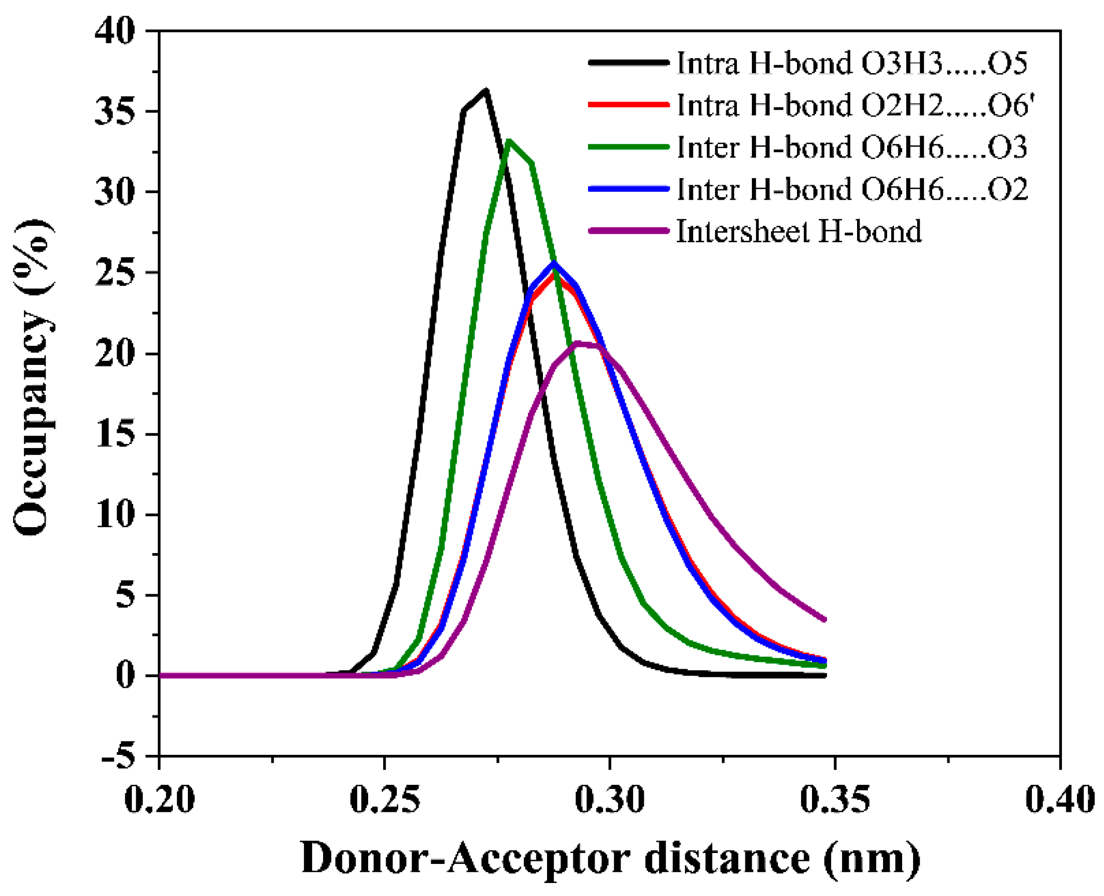
| Intra H-Bond O3H3…..O5 | Intra H-Bond O2H2…..O6’ | Inter H-Bond O6H6…..O3 | Inter H-Bond O6H6…..O2 | Intersheet H-Bond | ||||||
|---|---|---|---|---|---|---|---|---|---|---|
| Electric Field (mV/nm) | Bond length (nm) | Occupancy (%) | Bond length (nm) | Occupancy (%) | Bond length (nm) | Occupancy (%) | Bond length (nm) | Occupancy (%) | Bond length (nm) | Occupancy (%) |
| No field | 0.2725 | 36.32 | 0.2875 | 24.86 | 0.2775 | 33.18 | 0.2875 | 25.61 | 0.2925 | 20.62 |
| 0.001 | 0.2725 | 36.22 | 0.2875 | 24.88 | 0.2775 | 32.47 | 0.2875 | 25.34 | 0.2925 | 20.13 |
| 0.005 | 0.2725 | 36.09 | 0.2875 | 24.61 | 0.2775 | 32.82 | 0.2875 | 25.18 | 0.2925 | 19.65 |
| 0.01 | 0.2725 | 36.43 | 0.2875 | 24.79 | 0.2775 | 32.81 | 0.2875 | 25.37 | 0.2925 | 20.33 |
| 0.06 | 0.2725 | 36.17 | 0.2875 | 24.79 | 0.2775 | 33.06 | 0.2875 | 25.39 | 0.2975 | 19.94 |
| 0.09 | 0.2725 | 36.38 | 0.2875 | 24.93 | 0.2775 | 33.64 | 0.2875 | 25.76 | 0.2975 | 20.55 |
| 0.2 | 0.2725 | 36.16 | 0.2875 | 24.66 | 0.2775 | 32.37 | 0.2875 | 25.26 | 0.3375 | 29.59 |
| 0 ns | 2 ns | 4 ns | 6 ns | 8 ns | 10 ns | 12 ns | 14 ns | 16 ns | 18 ns | 20 ns |
|---|---|---|---|---|---|---|---|---|---|---|
| 1 mV/nm | ||||||||||
 | ||||||||||
| 2 mV/nm | ||||||||||
 | ||||||||||
| 4.5 mV/nm | ||||||||||
 | ||||||||||
Publisher’s Note: MDPI stays neutral with regard to jurisdictional claims in published maps and institutional affiliations. |
© 2022 by the authors. Licensee MDPI, Basel, Switzerland. This article is an open access article distributed under the terms and conditions of the Creative Commons Attribution (CC BY) license (https://creativecommons.org/licenses/by/4.0/).
Share and Cite
Muthoka, R.M.; Panicker, P.S.; Kim, J. Molecular Dynamics Study of Cellulose Nanofiber Alignment under an Electric Field. Polymers 2022, 14, 1925. https://doi.org/10.3390/polym14091925
Muthoka RM, Panicker PS, Kim J. Molecular Dynamics Study of Cellulose Nanofiber Alignment under an Electric Field. Polymers. 2022; 14(9):1925. https://doi.org/10.3390/polym14091925
Chicago/Turabian StyleMuthoka, Ruth M., Pooja S. Panicker, and Jaehwan Kim. 2022. "Molecular Dynamics Study of Cellulose Nanofiber Alignment under an Electric Field" Polymers 14, no. 9: 1925. https://doi.org/10.3390/polym14091925
APA StyleMuthoka, R. M., Panicker, P. S., & Kim, J. (2022). Molecular Dynamics Study of Cellulose Nanofiber Alignment under an Electric Field. Polymers, 14(9), 1925. https://doi.org/10.3390/polym14091925