Abstract
Carbon dioxide (CO2)-assisted polymer compression method is used for plasticizing polymers with subcritical CO2 and then crimping the polymer fibers. Given that this method is based on crimping after plasticization by CO2, it is very important to know the degree of plasticization. In this study, heat treatment was gently applied on raw material fibers to obtain fibers with different degrees of crystallinity without changing the shape of the fibers. Simultaneously, two types of sheets were placed in a pressure vessel to compare the degree of compression and the degree of hardness. Furthermore, a model was used to derive the relative Young’s modulus of porous materials composed of polymer fibers with different degrees of crystallinity. In the model, the amount of strain was calculated according to the Young’s modulus as a function of porosity and reflected in compression. Young’s modulus of porous polymers in the presence of CO2 has been shown to vary significantly with slight differences in crystallinity, indicating that extremely low crystallinity is significant for plasticizing the polymer by CO2.
1. Introduction
CO2 is a gas with low toxicity and is being used in the food [1] and pharmaceutical industries [2]. CO2 is known to specifically dissolve in polymers, and research on the mixture of polymers and CO2 has been actively conducted in relation to the polymer process [3] and polymer synthesis [4]. The dissolution of CO2 in solid [5] or melted polymers [6] has been used in the foaming process. The rapid expansion of supercritical solution [7], particles from gas saturated solutions [8], and supercritical antisolvent methods [9] have been proposed as processes that use CO2 to atomize the polymer.
Under these circumstances, the CO2-assisted polymer compression (CAPC) method, which is a method used to produce porous material by plasticizing and crimping polymer fibers with CO2 under subcritical conditions of vapor pressure at room temperature, was developed [10]. The process leads to the creation of porous materials with through holes in a short time. Until now, the CAPC method has been focused on properties and process conditions for practical use, such as porosity and pore diameter [11], adhesion strength [12], controlled release [13], air permeability [14], and mass production [15]. Recently, utility components, such as multilayer filters (considerations with classical model [16], considerations with deep-learning model [17]), application to bioplastics [18], and creation of reaction cartridges loaded with enzymes [19], have been developed. The CAPC method is used at room temperature. The method has the limitation that the polymers need to be plasticized under subcritical conditions, which are gentler than supercritical conditions. In other words, to understand the applicability of the CAPC method, one needs to understand the plasticization of the polymers involved. CO2 is known to easily dissolve into polymers, especially when dissolved in the amorphous part, by numerous viewpoints (reaction engineering of polymers in supercritical CO2 [20], model calculations of CO2 solubility [21], determination of CO2 solubility [22], and interaction between polymers and CO2 [23]). The degree of crystallinity of the polymers greatly affects the formation of foams by influencing the solubility and diffusion of CO2 [24]. In the case of semicrystalline polymers, the crystalline state of the polymer affects the nucleation of foam [25], and several approaches to strategically use such polymers to create foams have also been attempted [26]. Thus, there are many cases where solid polymers and CO2 processes require the consideration of crystallinity and crystalline state.
The crimping of fibers by the CAPC method does not occur in the absence of CO2. As a result, the plasticization of the polymer by CO2 is known to be essential. From previous studies, the plasticization of polymers by CO2 would be affected by the degree of crystallinity of the polymer. However, the effect must be evaluated using the measurement of Young’s modulus under high pressure, and there has only been a little research conducted on this topic. In the case of fibrous porous polymers, such as in the CAPC method, unless the fiber diameters are matched, it is impossible to observe only the effect of crystallinity, and unless the resin is made from the same pellets, it is not easy to observe only the effect of crystallinity because the resin may be affected by some other components, such as molecular weight distribution.
In this study, these problems have been solved by cold crystallization of polyethylene terephthalate (PET) nonwoven sheets by heat treating them for a given period above the glass transition point without changing the shape of the fibers and by adjusting samples with different degrees of crystallinity. Furthermore, analysis of Young’s modulus, both large and small, was carried out by piling up raw material sheets with different crystallinity values and placing them in a container to analyze how they crumpled after compression. The Young’s modulus for the porosity of the samples with different crystallinity was successfully obtained by analyzing the compression process with a model.
2. Materials and Methods
2.1. Materials
Nonwoven fabrics (average fiber diameter: 8 µm, basis weight: 30 g/m2) made by the melt blowing method [27] at Nippon Nozzle Co., Ltd. (Kobe, Japan) using PET pellets of TK3 (density: 1.34 g/mL) from Bell Polyester Products, Inc. (Houfu, Japan) were used as raw material fibers. The untreated samples were used as they were, while the samples with increased crystallinity were created by heat treating at 94 °C for 1.5 or 3 h to increase crystallinity without changing the fiber shape by gentle cold crystallization. The degree of crystallinity was checked by differential scanning calorimetry (DSC) on Thermo Plus Evo DSC 8230 (Rigaku Corporation, Akishima, Japan) under DSC measurement conditions of 9.39–10.40 mg sample weight and a temperature rise rate of 5 °C/min. The X-ray diffraction (XRD) profile of the untreated sample was measured by SmartLab (Rigaku Corporation, Akishima, Japan).
The untreated and heat-treated samples were punched at Φ18 mm to make circular samples. All the samples were aligned to 32 sheets of 0.253 g and neatly stacked to form a cylindrical shape. This shape was then used as one set of samples.
2.2. Compression Evaluation Method
A schematic diagram of the experimental setup is shown in Figure 1. The sample was prepared in a high-pressure vessel with a separator in the middle of the vessel and samples placed on top of the separator and below the separator. The piston was lowered to a position where the total thickness of the layers of the sample, excluding the separator, was 4 mm. The introduction of CO2 and exhaustion of O2 were repeated three times while controlling the V1 and V2 valves to replace the air in the high-pressure vessel with only CO2. Afterward, CO2 was introduced, and the piston was lowered to the press position. The position where the total thickness of the sample layer was recorded was at a height of 2.0–3.6 mm of the vessel. After holding the piston in the press position for 10 s, the exhaust valve V3 was opened and the gas was exhausted for 30 s through the metering valve V4, and then the V2 valve was opened to release the air. The samples were removed by raising the piston, and the center thickness of each sample was measured with a micrometer. This experiment was conducted at room temperature of 22 °C and the CO2 was introduced at a pressure of 6 MPa. The experiment was performed twice with one sample on top of the separator and twice with the same sample below the separator. The average of these four experiments was used. The surfaces of some samples were observed with a scanning electron microscope (SEM) TM-1000 (Hitachi High-Tech Co., Minato-ku, Japan).
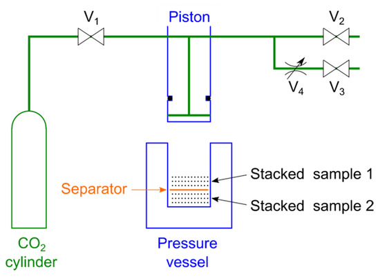
Figure 1.
Experimental equipment diagram. The pressure vessel and the piston are sealed with an O-ring on the side of the piston. The samples are put with a separator sandwiched between layers so that the layers do not stick to each other. V1: introduction valve; V2: high-speed exhaust valve; V3: low-speed exhaust valve; V4: metering valve.
2.3. Compression Calculation
The model for compression analysis used in the calculations was constructed when designing the multilayer filter [16]. The following relationship is established between the stress σ, Young’s modulus E, and strain ε of a material.
Young’s modulus is a function of porosity p. When two layers are present, as shown in Stacked sample 1 and Stacked sample 2 in Figure 2, the stress in each layer is demonstrated by the following equations:
where the subscripts 1 and 2 indicate layer 1 and layer 2, respectively. In the case of a two-layer sample stacked in a cylindrical shape, if the cross-sections are the same and the stresses (σ1 and σ2) are equal, the following relationship is established between Young’s modulus and the strain of each layer.
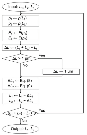
Figure 2.
Flowchart of calculating compression. Inputs are L1: thickness before compression of layer 1, L2: thickness before compression of layer 2, and Lf: total thickness after compression. Output is L1: thickness of compression of layer 1 and L2: thickness of layer 2 after compression. Function p is used to find the porosity from the thickness. The porosity is derived by calculating the bulk density from the thickness and then applying Equation (10). Function E is used to obtain Young’s modulus from porosity.
When the two layers are combined and compressed with total compression thickness, ΔL, the following relationship is established between the strains in each layer and their sum.
where L1 and L2 are the thicknesses of layer 1 and layer 2, respectively. Solving Equations (4)–(7), the amount of compression for each layer is as follows:
In the case of porous materials, Young’s modulus is known to have porosity dependence. Given that porosity changes as the material is compressed, the above equations are not valid when the compression amount is large. However, the above equations are adaptable when the strain is so small that the dependence on porosity becomes negligible. For this reason, in the previous report, the compression in the calculation was done in 1 µm steps, and the final compression state was calculated by repeating the micro-compression until a given thickness was achieved while updating Young’s modulus. Given that the outer diameter (Φ18 mm) and weight of the sample (0.253 g) were known, the bulk density ρporous of the cylindrical porous material could be easily calculated from the thickness. The difference between ρporous and ρsolid, the density of the nonporous material (1.34 g/mL), is the pore, and the porosity p of the material can be calculated by dividing this difference by ρsolid, which is shown in the following equation:
As the samples used in this study were those with slightly different crystallinity using the same polymer material, the solid densities of the used models could be considered identical, with an adequate precision of 1.34 g/mL.
The flowchart of the calculation is shown in Figure 2. The input parameters are the initial thickness of the first layer L1, the initial thickness of the second layer L2, and the final thickness Lf, while the output parameters are the thickness of the first layer after compression L1 and the final thickness of the second layer L2. From the flowchart, the sum of the outputs L1 and L2 is equal to the input Lf.
However, this analysis was limited by the fact that the distribution ratio of compression between the two layers is determined by the ratio of Young’s modulus between them, so the absolute values of Young’s modulus of each of the two layers were not determined. Therefore, only the ratio of Young’s modulus was determined, which is a relative index.
2.4. Determination of Crystallinity
The crystallinity of the samples was determined by DSC. The degree of crystallinity from the DSC profile is determined by the following equation [28]:
where ΔHc1 and ΔHc2 are the enthalpies of cold crystallization and ΔH0 is the fusion enthalpy of a fully crystallized sample, which has been reported to be 140 J/g for PET [29]. Research has been conducted to apply this formula to PET [30]. In the present system, ΔHc2 and ΔHm overlap; however, the value ΔHc2 + ΔHm can be determined by taking the integral of the overlapped state. If ΔHc2 + ΔHm is denoted by , subsequently, Equation (11) becomes
3. Results and Discussion
The DSC profiles of the nonwoven fabric before heat treatment, after heat treatment for 1.5 h, and after heat treatment for 3 h are shown in Figure 3. Two peaks of cold crystallization were observed around 125 °C and 250 °C, and the peak of fusion was observed around 260 °C. The position of the cold crystallization peak varied depending on the state of the amorphous part. The case of two cold crystallization peaks was observed in other systems as well [31].
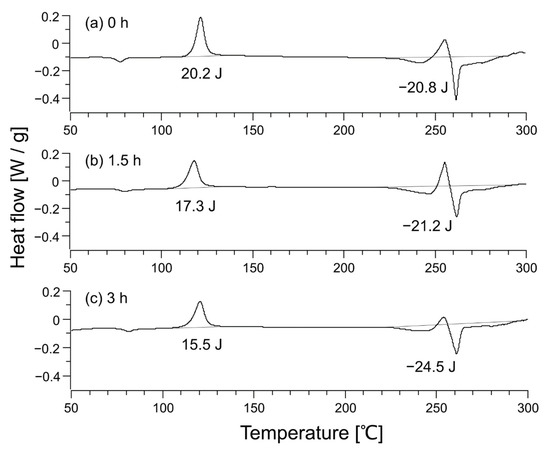
Figure 3.
Differential scanning calorimetry profile of unheated sample (a), sample after heat treatment for 1.5 h (b), and sample after heat treatment for 3 h (c). The heat flow in the chart is positive for an exothermic reaction, so the enthalpies listed in the figure correspond to and in Equation (12).
Using Equation (12), the crystallinity of each sample was calculated to be 0.4% for the untreated nonwoven fabric, 2.8% for the nonwoven fabric heat-treated for 1.5 h, and 6.4% for the nonwoven fabric heat-treated for 3 h. The XRD profiles of nonwoven fabrics are shown in Figure 4. The XRD profile of the polymer shows a broad halo for the amorphous part and a sharp peak for the crystalline part [32]. However, no sharp peaks were observed in Figure 4a, indicating that the crystallinity was close to zero, which is consistent with the DSC result of 0.4% crystallinity for the untreated nonwoven fabric. Figure 4c depicts small peaks overlapping the broad halo, showing a slight crystallization, consistent with the 6.4% crystallinity determined from DSC.
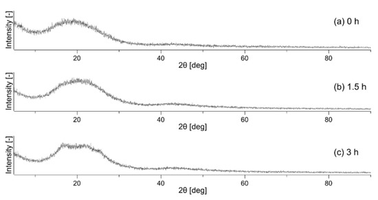
Figure 4.
X-ray diffraction profile of unheated sample (a), sample after heat treatment for 1.5 h (b), and sample after heat treatment for 3 h (c).
SEM images of raw nonwoven fabrics are shown in Figure 5a–c. The observation results of the fiber surface when only one type of sample was placed, CO2 was introduced at 2 mm, and the sample was compressed to 1 mm are shown in Figure 5d–f. No foaming was observed on the fiber surface because supercritical conditions were not used, the time of exposure to CO2 was short, and the fiber diameter was small enough such that the dissolved CO2 could easily exit from the fiber. The CO2 emitted from the fibers was exhausted through the void between the fibers, so the resulting porous material had through holes. Traces of crushing by the piston were observed on the surface of the fibers, and the press marks on the surface became slightly larger in the order of 3 h treatment, 1.5 h treatment, and untreated, suggesting that the fibers were more crushed. However, the SEM images did not show a clear enough difference to identify the hardness of the fibers.
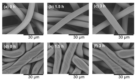
Figure 5.
Scanning electron microscope images of the surface of raw nonwoven fabrics and the sample compressed to 1 mm. (a) Raw nonwoven fabric without heat treatment, (b) raw nonwoven fabric after 1.5 h heat treatment, (c) raw nonwoven fabric after 3 h heat treatment, (d) CO2-assisted polymer compression (CAPC) product made from untreated nonwoven fabric, (e) CAPC product using nonwoven fabric heated at 94 °C for 1.5 h as raw material, and (f) CAPC product using nonwoven fabric heated at 94 °C for 3 h as raw material.
The results of the two-layer compression test are shown in Table 1. The experiments were conducted under 15 different experimental conditions: A1–A5, B1–B5, and C1–C5. Experiment A1 was conducted with a combination of non-heat-treated nonwoven fabric (heat treatment time: 0 h) and 1.5 h heat-treated nonwoven fabric. When compressed with a piston from the 4 mm CO2 introduction position, the layer of non-heat-treated nonwoven fabric was compressed to 1.774 mm, whereas the layer of 1.5 h heat-treated nonwoven fabric was compressed to 1.825 mm. Similarly, Experiment A2 was conducted with the combination of non-heat-treated nonwoven fabric (heat treatment time: 0 h) and 1.5 h heat-treated nonwoven fabric. When compressed with a piston from the 4 mm CO2 introduction position, the 0 h nonwoven fabric layer was compressed to 1.557 mm, whereas the 1.5 h heat-treated nonwoven fabric layer was compressed to 1.645 mm. As written in the experiment section, two experiments with one of the two types of samples on top and two experiments with the same type of samples on the bottom, making it a total of four experiments, were conducted. The mean values and standard deviations are shown in Table 1. No difference was recorded between the experiments with the sample on top and those with the sample on the bottom, and there was no dependence of the experiment on the position of the sample. In all experiments, the untreated samples were more compacted than the 1.5 h heat-treated samples, and the 1.5 h heat-treated samples were more compacted than the 3 h heat-treated samples, indicating that the hardness increased in the order of untreated, 1.5 h heat-treated, and 3 h heat-treated samples. This increasing order of hardness of the samples is consistent with the order of crystallinity, suggesting that the degree of plasticization decreases in the order of untreated, 1.5 h heat-treated, and 3 h heat-treated samples. This order of the degree of plasticization is consistent with those of amorphous area, showing that plasticization is caused by the impregnation into the amorphous part of the polymer.

Table 1.
Experimental results and model calculation results.
Model calculation was performed to derive the relationship between the porosity and Young’s modulus of the porous material in the presence of CO2. Although the initial thickness of the porous material is necessary for the model calculation, the thickness of each layer in the initial state when each layer of the nonwoven fabric is placed in a stack and compressed by a piston could not be ascertained because the stainless steel container was opaque. Therefore, the following considerations were obtained. The position of CO2 introduction was the same regardless of the experimental conditions, so for example, Experiment A2 was considered to have been reached after going through the state of Experiment A1 during the compression process by the piston. Similarly, Experiment A3 was considered to have been reached after going through the state of Experiment A1 and that of Experiment A2. When the state before the final state was known, the result of Experiment A1 could be used as the initial value for the calculation performed to compress the final state to the total value of each layer of Experiment A2, and then to check how well the result agreed with the experimental result. Similarly, for Experiment A3, the result of Experiment A2 was used as the initial value for the calculation performed to compress the final state to the total value of each layer of Experiment A3. This operation was performed for each experiment, and fitting was performed so that the least-squares error between the experimental and calculated values would be small. The parameters were determined using the Nelder–Mead method [33], which does not require derivation of derivatives for fitting. In incorporating the Nelder–Mead method into the program, Reference [34] was employed. The fitting of the results was performed on only 12 out of the 15 datasets (A2–A5, B2–B5, C2–C5) because the model calculation used the previous data to establish the initial value. The number of fitting parameters varied from two to four, depending on the equation to be fitted, and the amount of fitting data required was sufficiently larger than the amount of fitting parameters.
The Young’s modulus of the CAPC product was calculated by conversion from hardness measurement [35]. Several equations have been proposed for the elastic modulus of porous materials, such as ceramics [36], metals [37], and unspecified materials [38]. These equations are largely classified into those with and without critical porosity. However, in a previous paper [35], the following simple equation without critical porosity was presented:
where Young’s modulus E0 of the solid without pore was 266 MPa and the shape factor f was 2.41. Equation (13) is for the case when CO2 is removed after CAPC and the material returns to its unplasticized state. Assuming that the shape of the curve is unaltered in the presence of CO2 and only the absolute value changes, Young’s modulus as a function of porosity was assumed to be the following equations:
The parameters C1.5h and C3h were determined using the least-squares method. In Equation (14), Young’s modulus is 1 when the porosity of the untreated sample is 0. This outcome is because this method can only determine the relative value of Young’s modulus. The Young’s modulus determined by this method is shown in Figure 6. In Figure 6, Young’s modulus is plotted for a limited porosity range because Young’s modulus is plotted for the porosity only in the fitting range. The results of the calculations are shown in Table 1, where the value of the coefficient of determination R2 was 0.9928.
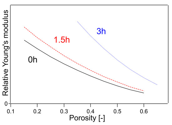
Figure 6.
Young’s modulus fitted by Equations (14)–(16). The numbers in the figure indicate the heating time of the sample.
As in the previous study [16], which fabricated a multilayer filter using the same untreated nonwoven fabric used in this study, Young’s modulus was determined to simulate the thickness of each layer. In addition, a fifth-order polynomial was used to fit the results. These results, fitted by the fifth-order polynomial and the result of fitting with Equation (13), are shown in Figure 7. These results agree extremely well with the general porosity and Young’s modulus equations, and the fitting parameter f was 4.77 at that time. Therefore, the following equations using this parameter f = 4.77 were used as the next trial.
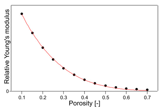
Figure 7.
The plot of the quintic function used when designing the multilayer filter [16] and the fitting result with Equation (13).
The results are shown in Table 1 and Figure 8. The value of R2 was 0.9944, which was better than the previous result using Equations (14)–(16), indicating that Young’s modulus trend in the presence of CO2 was still slightly different from that in the absence of CO2.
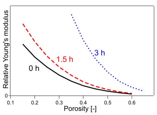
Figure 8.
Young’s modulus fitted by Equations (17)–(19). The numbers in the figure indicate the heating time of the sample.
Here, a question arose as to whether the functional form of Young’s modulus in the presence of CO2 would be the same regardless of the degree of crystallinity. The previously reported functional form was for the untreated sample. Therefore, Young’s modulus was calculated using the following equations:
In Equations (20)–(22), the exponential part of the function was fixed only for the untreated sample, whereas the exponential part of each of the remaining samples was used as the fitting parameter. The results are shown in Table 1 and Figure 9. The value of R2 was 0.9987, which was a significant improvement. The results of the fitting parameters were as follows: C1.5h was 1.01, C3h was 1.55, f1.5h was 4.26, and f3h was 3.14. C1.5h and C3h represent the Young’s modulus of a solid without pores, showing that the Young’s modulus of a sample with 2.8% crystallinity was 1.01 and that with 6.4% crystallinity was 1.55, when the crystallinity of the sample with 0.4% crystallinity was 1. The f1.5h and f3h are shape factors. In the case of the present sample, because the fibers were stacked horizontally and compressed, the elastic modulus was considered a mixture of tensile and flexural modulus. The contribution of flexural modulus was expected to be larger on the low-density sample, and the contribution of tensile modulus was expected to be larger as it approached high-density pore-free solids. It is well known that the flexural modulus is generally lower in value than the tensile modulus of elasticity for practical purposes [39]. In the present case, the effect of mixing the tensile and flexural modulus was included in the shape factor, and the shape factor was regarded to have changed with crystallinity. As the degree of crystallinity increased, the functional form approached that of Young’s modulus of the CAPC porous material (f = 2.41) after CAPC treatment. Figure 9 shows that Young’s modulus increases in the order of untreated, 1.5 h heat-treated, and 3 h heat-treated samples, indicating the increasing hardness of the material in that order. In particular, comparing Young’s modulus of untreated and 3 h heat-treated specimens, Young’s modulus of 3 h heat-treated specimens with a porosity of 0.4 was about four times higher than that of untreated specimens, and Young’s modulus of 3 h heat-treated specimens with a porosity of 0.5 was about five times higher than that of untreated specimens, indicating a large difference.
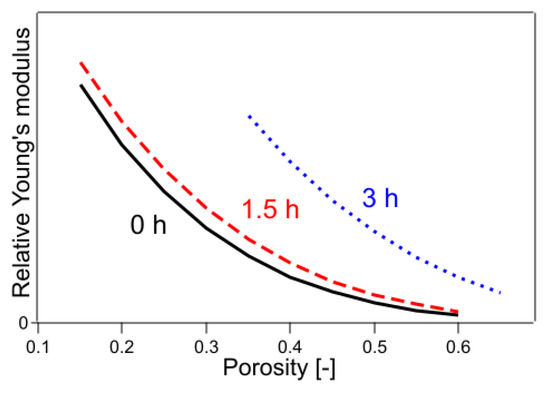
Figure 9.
Young’s modulus fitted by Equations (20)–(22). The numbers in the figure indicate the heating time of the sample.
The present results show that Young’s modulus of CAPC porous materials in the presence of CO2 can be expressed in a very simple description without critical porosity, which can be used to describe the experimental results. It has also been shown that Young’s modulus changed significantly even after heat treatment for 3 h, although the degree of crystallinity at that time was as low as 6.4%. Considering that the categorization of the CAPC method is crimping, which is highly dependent on the hardness of the material selected, it is important to keep the crystallinity of the raw fiber very low and to use a material with a low Young’s modulus in the presence of CO2.
4. Conclusions
By heat treating the raw material fibers at low temperatures for a given period, samples with different degrees of crystallinity were prepared without changing the fiber shape. These samples were subjected to CAPC treatment in two overlapping layers, and the difference in compressibility of each layer was measured. The measured results were simulated using the analysis of strain by Young’s modulus. The relative magnitude of Young’s modulus of the samples with different crystallinity values and its functional form with respect to porosity were studied. It was shown that Young’s modulus of the porous polymer in the presence of CO2 changed significantly with a small difference in crystallinity, and that with increasing crystallinity, Young’s modulus approached the functional form in the atmosphere without CO2. Given that the degree of crystallinity of the nonwoven fabric made by the melt blowing method was extremely low, it can be inferred that the CAPC method is more effective if the nonwoven fabric in its state of low crystallinity after melt blowing is used as the raw fiber in its original state.
Funding
This research was supported by JSPS KAKENHI Grant Number 22H01379.
Institutional Review Board Statement
Not applicable.
Informed Consent Statement
Not applicable.
Data Availability Statement
All data generated or analyzed during this study are included in this published article.
Conflicts of Interest
The author declares no conflict of interest.
References
- Wang, W.; Rao, L.; Wu, X.; Wang, Y.; Zhao, L.; Liao, X. Supercritical carbon dioxide applications in food processing. Food Eng. Rev. 2021, 13, 570–591. [Google Scholar] [CrossRef]
- Balaban, M.O.; Ferrentino, G. Dense Phase Carbon Dioxide: Food and Pharmaceutical Apprications; Wiley, Blackwell: Ames, IA, USA, 2012; ISBN 978-0813806495. [Google Scholar]
- Tomasko, D.L.; Li, H.; Liu, D.; Han, X.; Wingert, M.J.; Lee, L.J.; Koelling, K.W. A review of CO2 applications in the processing of polymers. Ind. Eng. Chem. Res. 2003, 42, 6431–6456. [Google Scholar] [CrossRef]
- Boyère, C.; Jérôme, C.; Debuigne, A. Input of supercritical carbon dioxide to polymer synthesis: An overview. Eur. Polym. J. 2014, 61, 45–63. [Google Scholar] [CrossRef]
- Sarver, J.A.; Kiran, E. Foaming of polymers with carbon dioxide—The year-in-review–2019. J. Supercrit. Fluids 2021, 173, 105166. [Google Scholar] [CrossRef]
- Sauceau, M.; Fages, J.; Common, A.; Nikitine, C.; Rodier, E. New challenges in polymer foaming: A review of extrusion processes assisted by supercritical carbon dioxide. Prog. Polym. Sci. 2011, 36, 749–766. [Google Scholar] [CrossRef]
- Kumar, R.; Thakur, A.K.; Banerjee, N.; Chaudhari, P. A critical review on the particle generation and other applications of rapid expansion of supercritical solution. Int. J. Pharmaceutics 2021, 608, 121089. [Google Scholar] [CrossRef]
- Esfandiari, N. Production of micro and nano particles of pharmaceutical by supercritical carbon dioxide. J. Supercrit. Fluids 2015, 100, 129–141. [Google Scholar] [CrossRef]
- Yeo, S.-D.; Kiran, E. Formation of polymer particles with supercritical fluids: A review. J. Supercrit. Fluids 2005, 34, 287–308. [Google Scholar] [CrossRef]
- Aizawa, T. A new method for producing porous polymer materials using carbon dioxide and a piston. J Supercrit. Fluids 2018, 133, 38–41. [Google Scholar] [CrossRef]
- Aizawa, T. Fabrication of porosity-controlled polyethylene terephthalate porous materials using a CO2-assisted polymer compression method. RSC Adv. 2018, 8, 3061–3068. [Google Scholar] [CrossRef] [Green Version]
- Aizawa, T. Peel and penetration resistance of porous polyethylene terephthalate material produced by CO2-assisted polymer compression. Molecules 2019, 24, 1384. [Google Scholar] [CrossRef]
- Wakui, Y.; Aizawa, T. Analysis of sustained release behavior of drug-containing tablet prepared by CO2-assisted polymer compression. Polymers 2018, 10, 1405. [Google Scholar] [CrossRef]
- Aizawa, T.; Wakui, Y. Correlation between the porosity and permeability of a polymer filter fabricated via CO2-assisted polymer compression. Membranes 2020, 10, 391. [Google Scholar] [CrossRef]
- Aizawa, T. Process development of CO2-assisted polymer compression for high productivity: Improving equipment and the challenge of numbering-up. Technologies 2019, 7, 39. [Google Scholar] [CrossRef]
- Aizawa, T. Novel strategy for fabricating multi-layer porous membranes with varying porosity. ACS Omega 2020, 5, 24461–24466. [Google Scholar] [CrossRef]
- Aizawa, T. New design method for fabricating multilayer membranes using CO2-assisted polymer compression process. Molecules 2020, 25, 5786. [Google Scholar] [CrossRef]
- Aizawa, T. Application of CO2-assisted polymer compression to polylactic acid and the relationship between crystallinity and plasticization. Compounds 2021, 1, 75–82. [Google Scholar] [CrossRef]
- Aizawa, T.; Matsuura, S.-I. Fabrication of enzyme-loaded cartridges using CO2-assisted polymer compression. Technologies 2021, 9, 85. [Google Scholar] [CrossRef]
- Kemmere, M.F.; Meyer, T. Supercritical Carbon Dioxide in Polymer Reaction Engineering; Wiley-VCH: Weinheim, Germany, 2005; ISBN 978-3527310920. [Google Scholar]
- Li, M.; Zhang, J.; Zou, Y.; Wang, F.; Chen, B.; Guan, L.; Wu, Y. Models for the solubility calculation of a CO2/polymer system: A review. Mater. Today Commun. 2020, 25, 1012772. [Google Scholar] [CrossRef]
- Lee, J.K.; Yao, S.X.; Li, G.M.; Jun, M.B.G.; Lee, P.C. Measurement methods for solubility and diffusivity of gases and supercritical fluids in polymers and its applications. Polym. Rev. 2017, 57, 695–747. [Google Scholar] [CrossRef]
- Kikic, I. Polymer–supercritical fluid interactions. J. Supercrit. Fluids 2009, 47, 458–465. [Google Scholar] [CrossRef]
- Zhang, Z.-X.; Li, L.; Xin, Z.X.; Kim, J.K. Fabrication of fine-celled PP/ground tire rubber powder composites using supercritical carbon dioxide. Cell. Polym. 2011, 30, 111–136. [Google Scholar] [CrossRef]
- Ni, J.; Yu, K.; Zhou, H.; Mi, J.; Chen, S.; Wang, X. Morphological evolution of PLA foam from microcellular to nanocellular induced by cold crystallization assisted by supercritical CO2. J. Supercrit. Fluids 2020, 158, 104719. [Google Scholar] [CrossRef]
- Kwon, D.E.; Aregay, M.G.; Park, B.K.; Lee, Y.-W. Preparation of polyethylene terephthalate foams at different saturation temperatures using dual methods of supercritical batch foaming. Korean J. Chem. Eng. 2021, 38, 2560–2566. [Google Scholar] [CrossRef]
- Drabek, J.; Zatloukal, M. Meltblown technology for production of polymeric microfibers/nanofibers: A review. Phys. Fluids 2019, 31, 091301. [Google Scholar] [CrossRef]
- Fried, J.R. Polymer Science and Technology, 3rd ed.; Prentice Hall: Upper Saddle River, NJ, USA, 2014; ISBN 978-0137039555. [Google Scholar]
- Mehta, A.; Gaur, U.; Wunderlich, B. Equilibrium melting parameters of poly(ethylene terephthalate). J. Polym. Sci. Polym. Phys. Ed. 1978, 16, 289–296. [Google Scholar] [CrossRef]
- Karagiannidis, P.G.; Stergiou, A.C.; Karayannidis, G.P. Study of crystallinity and thermomechanical analysis of annealed poly(ethylene terephthalate) films. Eur. Polym. J. 2008, 44, 1475–1486. [Google Scholar] [CrossRef]
- Bruckmoser, K.; Resch, K. Effect of processing conditions on crystallization behavior and mechanical properties of poly(lactic acid) staple fibers. J. Appl. Polym. Sci. 2015, 132, 42432. [Google Scholar] [CrossRef]
- Young, R.J.; Lovell, P.A. Introduction to Polymers, 3rd ed.; CRC Press: Boca Raton, FL, USA, 2011; ISBN 978-0849339295. [Google Scholar]
- Nelder, J.A.; Mead, R. A simplex-method for function minimization. Comput. J. 1965, 7, 308–313. [Google Scholar] [CrossRef]
- Press, W.H.; Teukolsky, S.A.; Vetterling, W.T.; Flannery, B.P. Numerical Recipes 3rd Edition: The Art of Scientific Computing, 3rd ed.; Cambridge University Press: New York, NY, USA, 2007; ISBN 978-0521880688. [Google Scholar]
- Aizawa, T. Analysis of restitution coefficient and hardness of CO2-assisted polymer compression products. J. Chem. Eng. Jpn. 2021, 54, 463–466. [Google Scholar] [CrossRef]
- Kováčik, J. Correlation between Young’s modulus and porosity in porous materials. J. Mater. Sci. Lett. 1999, 18, 1007–1010. [Google Scholar] [CrossRef]
- Ternero, F.; Rosa, L.G.; Urban, P.; Montes, J.M.; Cuevas, F.G. Influence of the total porosity on the properties of sintered materials—A review. Metals 2021, 11, 730. [Google Scholar] [CrossRef]
- Choren, J.A.; Heinrich, S.M.; Silver-Thorn, M.B. Young’s modulus and volume porosity relationships for additive manufacturing applications. J. Mater. Sci. 2013, 48, 5103–5112. [Google Scholar] [CrossRef]
- Campo, E.A. Selection of Polymeric Materials: How to Select Design Properties from Different Standards; William Andrew: Norwich, NY, USA, 2008; ISBN 978-0815515517. [Google Scholar]
Publisher’s Note: MDPI stays neutral with regard to jurisdictional claims in published maps and institutional affiliations. |
© 2022 by the author. Licensee MDPI, Basel, Switzerland. This article is an open access article distributed under the terms and conditions of the Creative Commons Attribution (CC BY) license (https://creativecommons.org/licenses/by/4.0/).