
Manufacturing Polymer Model of Anatomical Structures with Increased Accuracy Using CAx and AM Systems for Planning Orthopedic Procedures

 ,
,  ,
,  ,
,  ,
,
Abstract
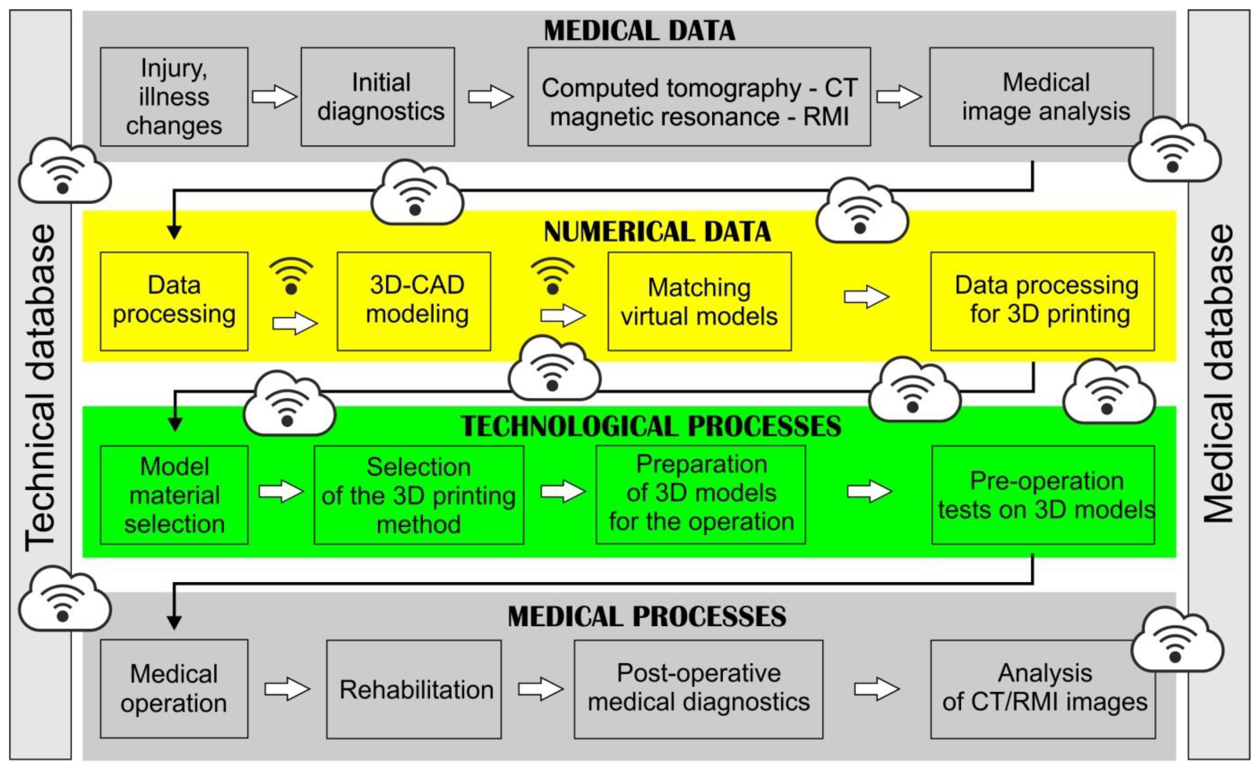
:1. Introduction
2. Materials and Methods
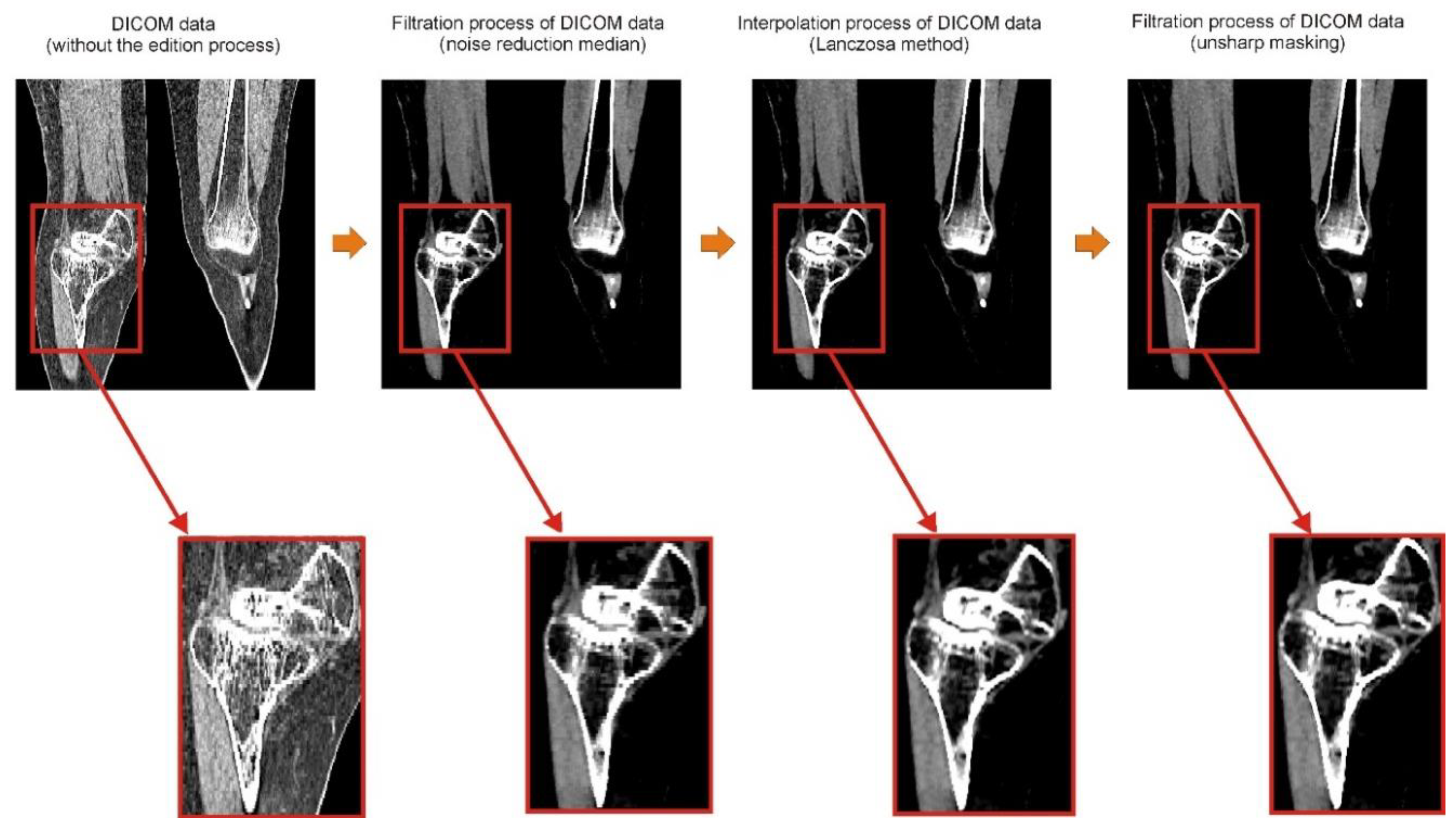
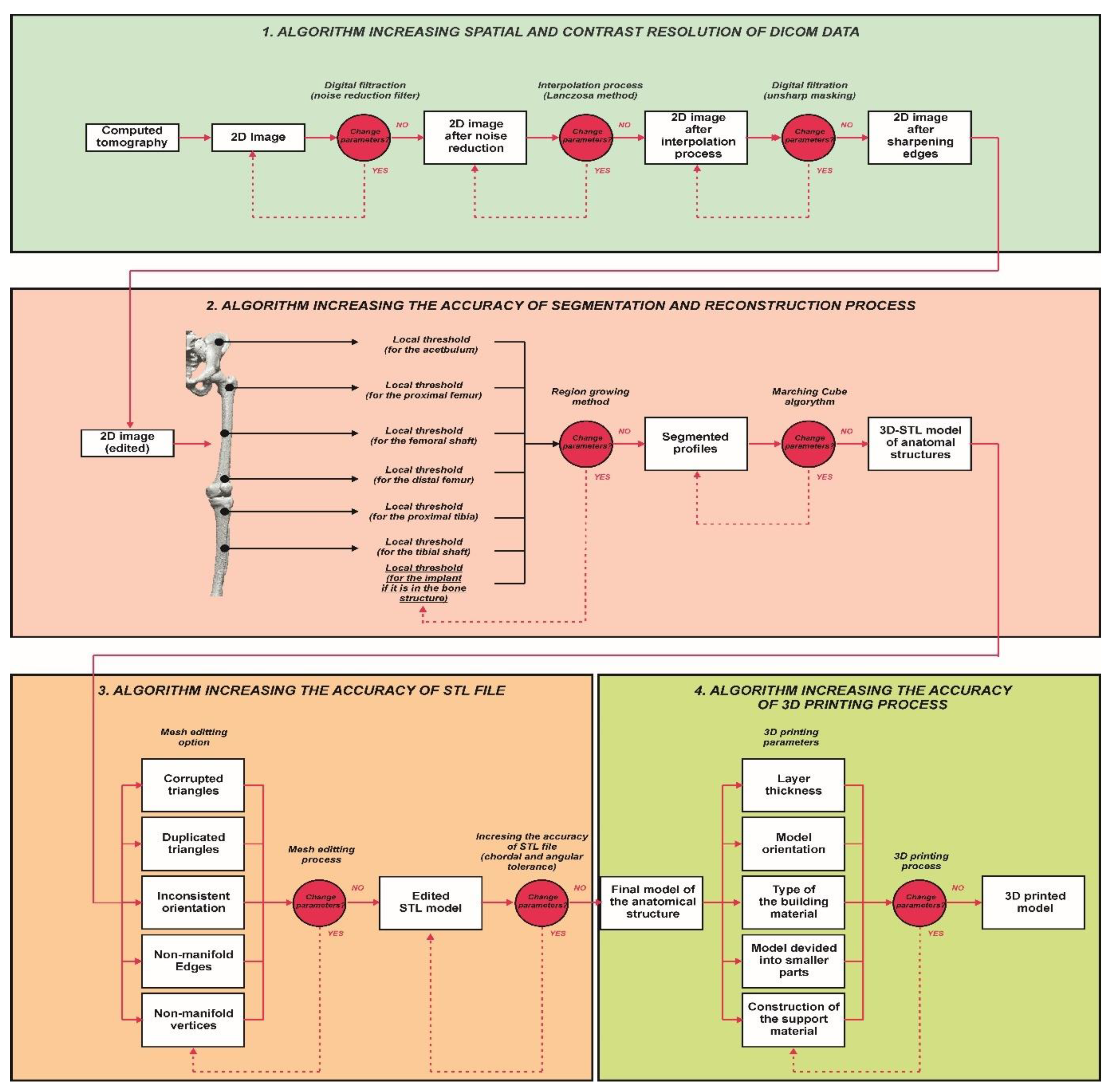
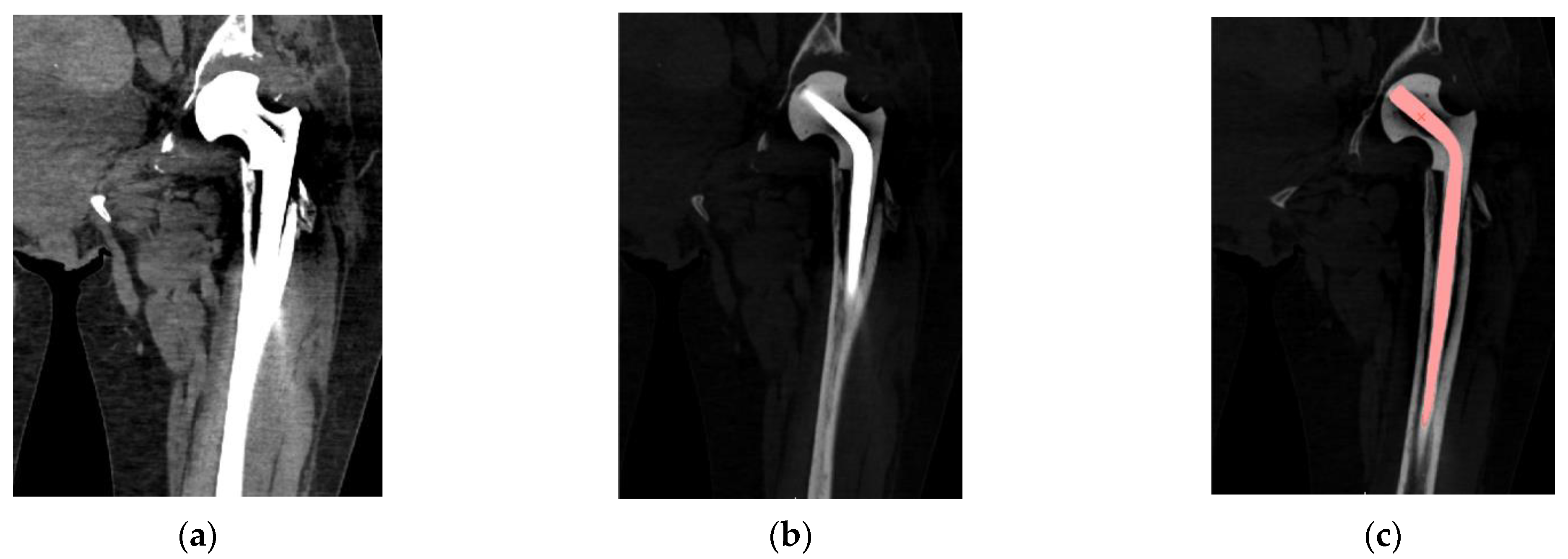
2.1. Digital Data Processing
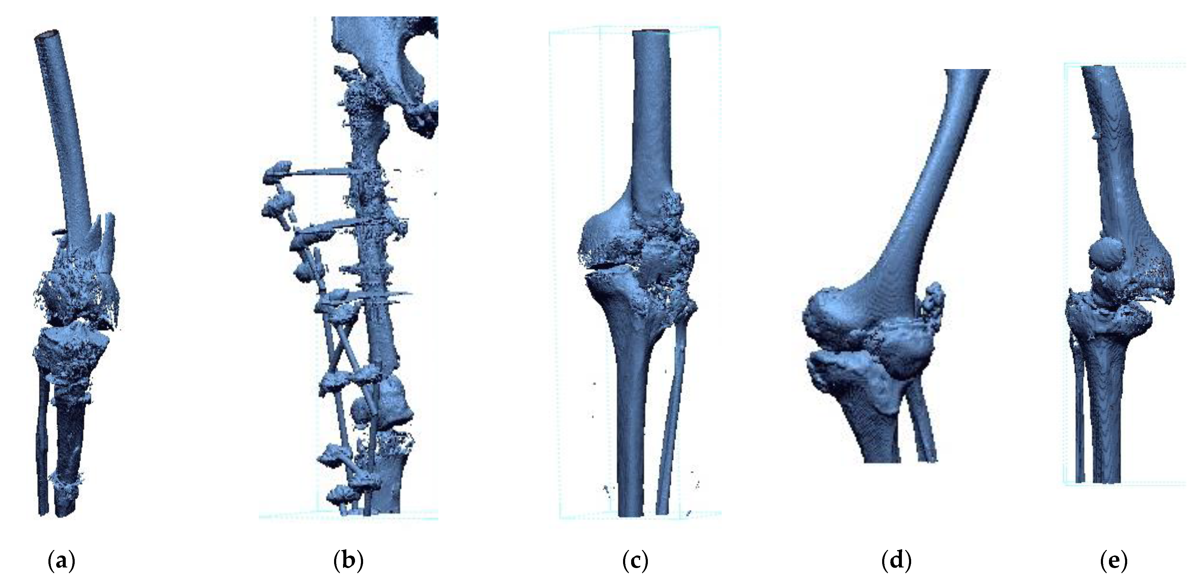
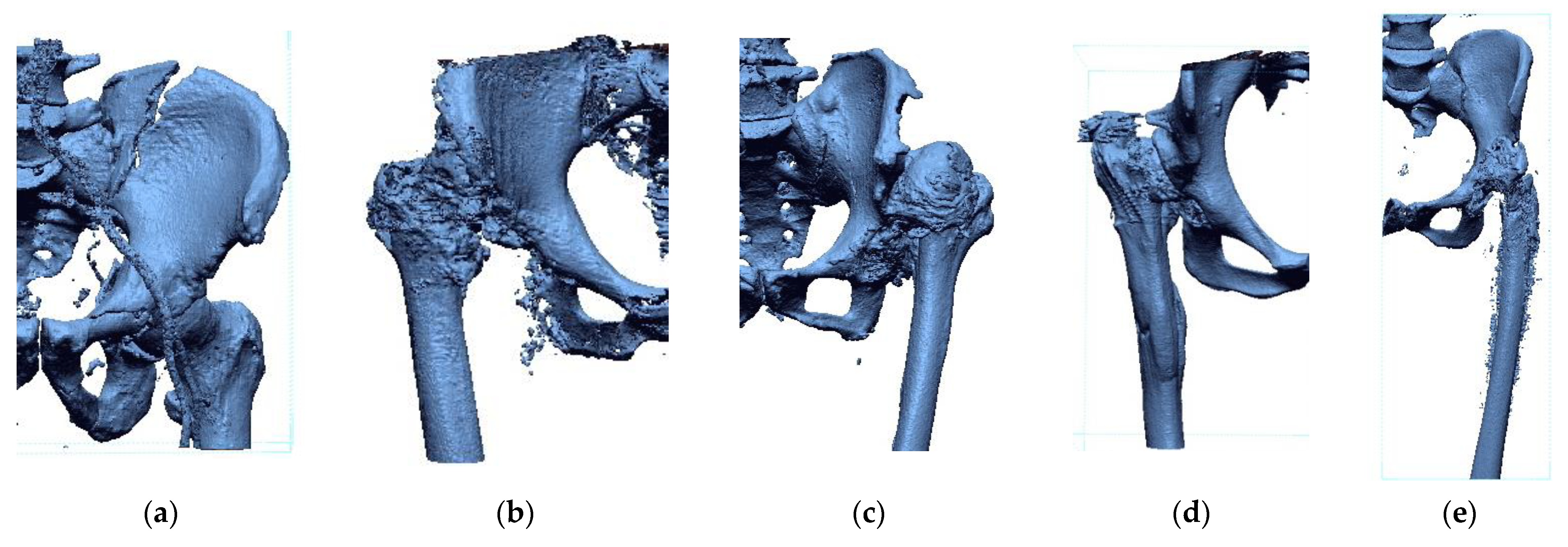
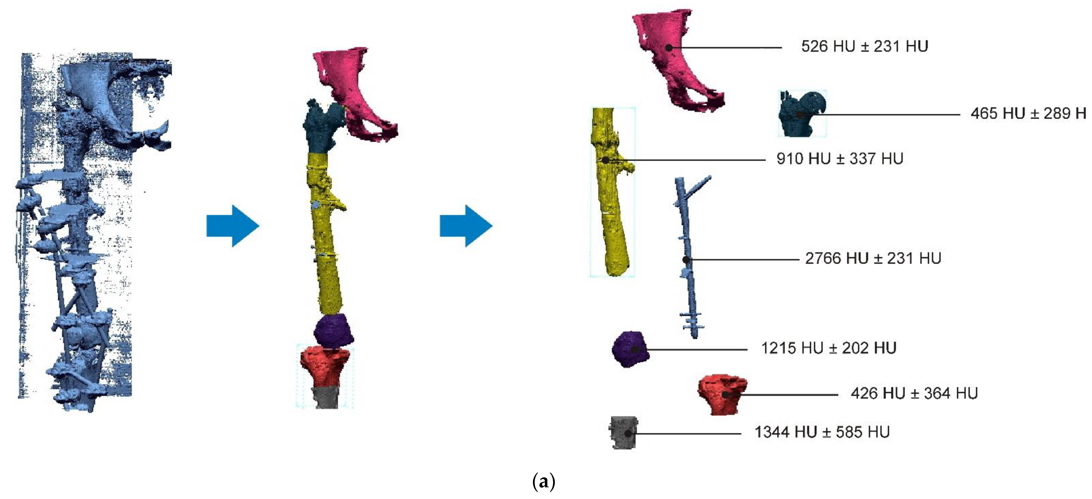
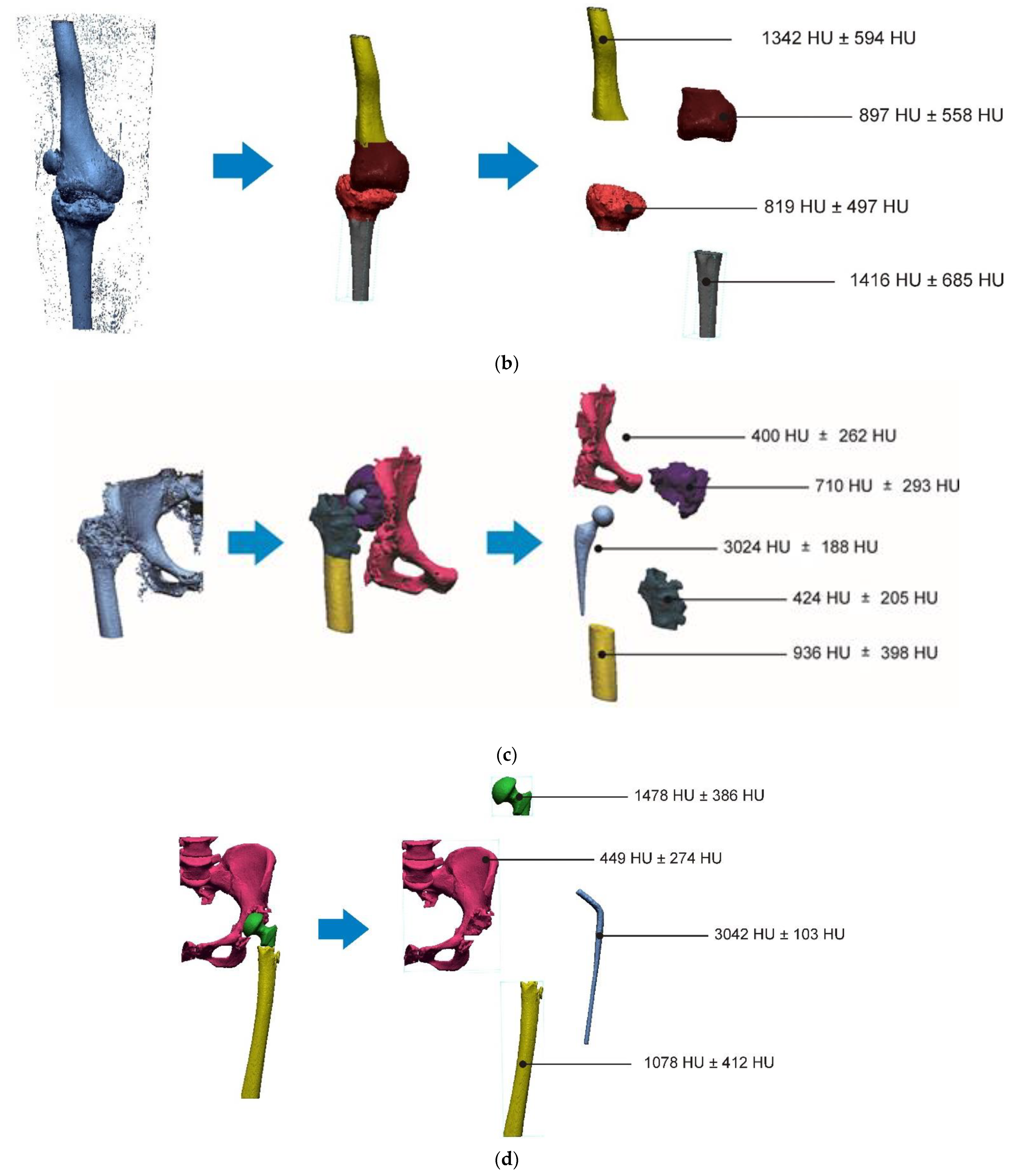
2.2. Segmentation and Reconstruction of the Geometry
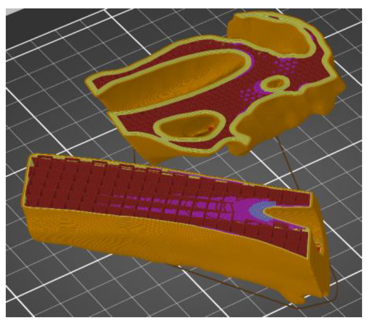
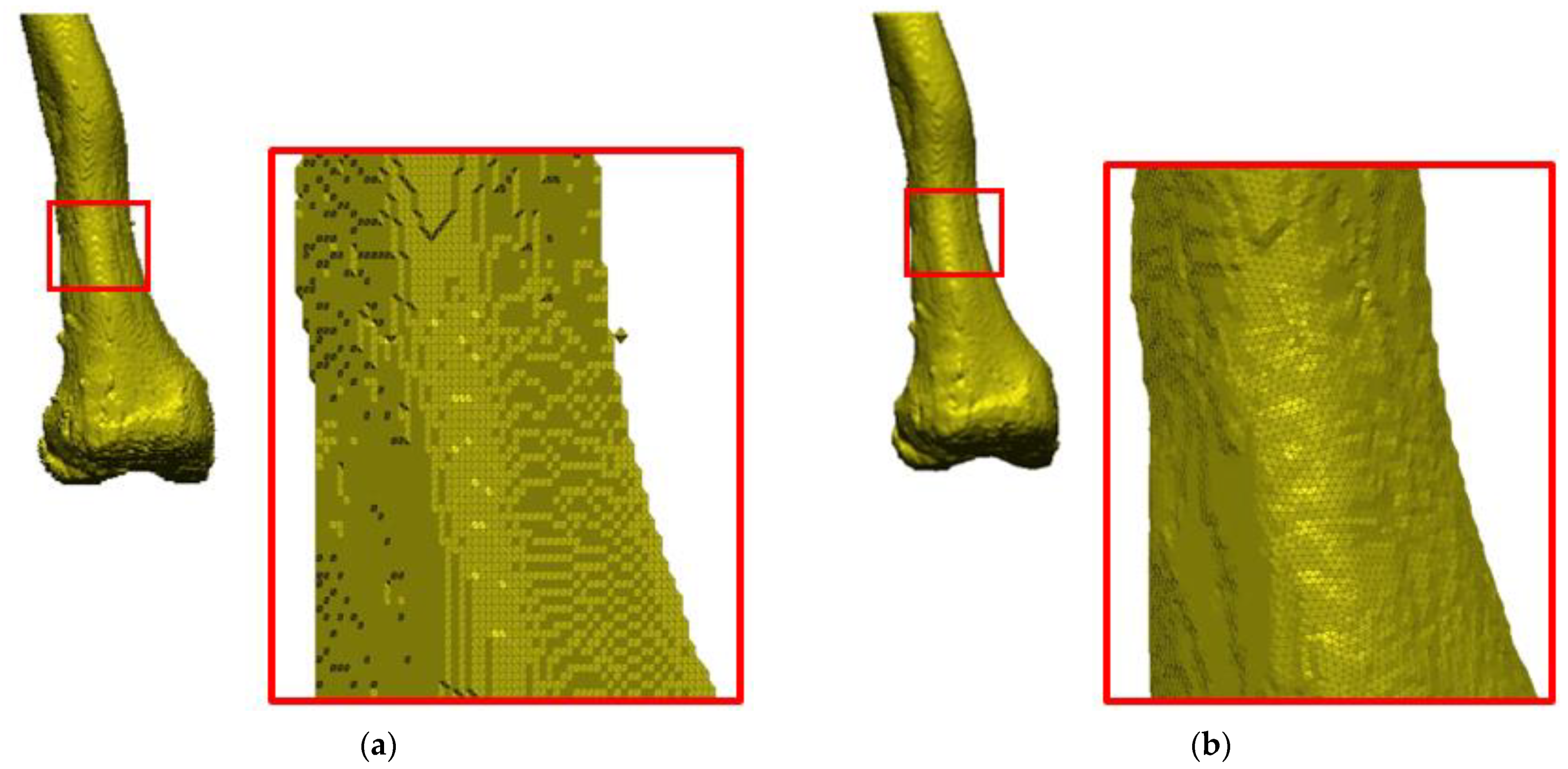
2.3. Increasing the Accuracy of the STL Model
- Normal vectors are inverted;
- Gaps between the triangles appear;
- Surface distortion;
- Lack of the entire surface or its selected fragments;
- Overlapping and intersecting triangles;
- No common edge;
- Addition of free triangles with no bounds.
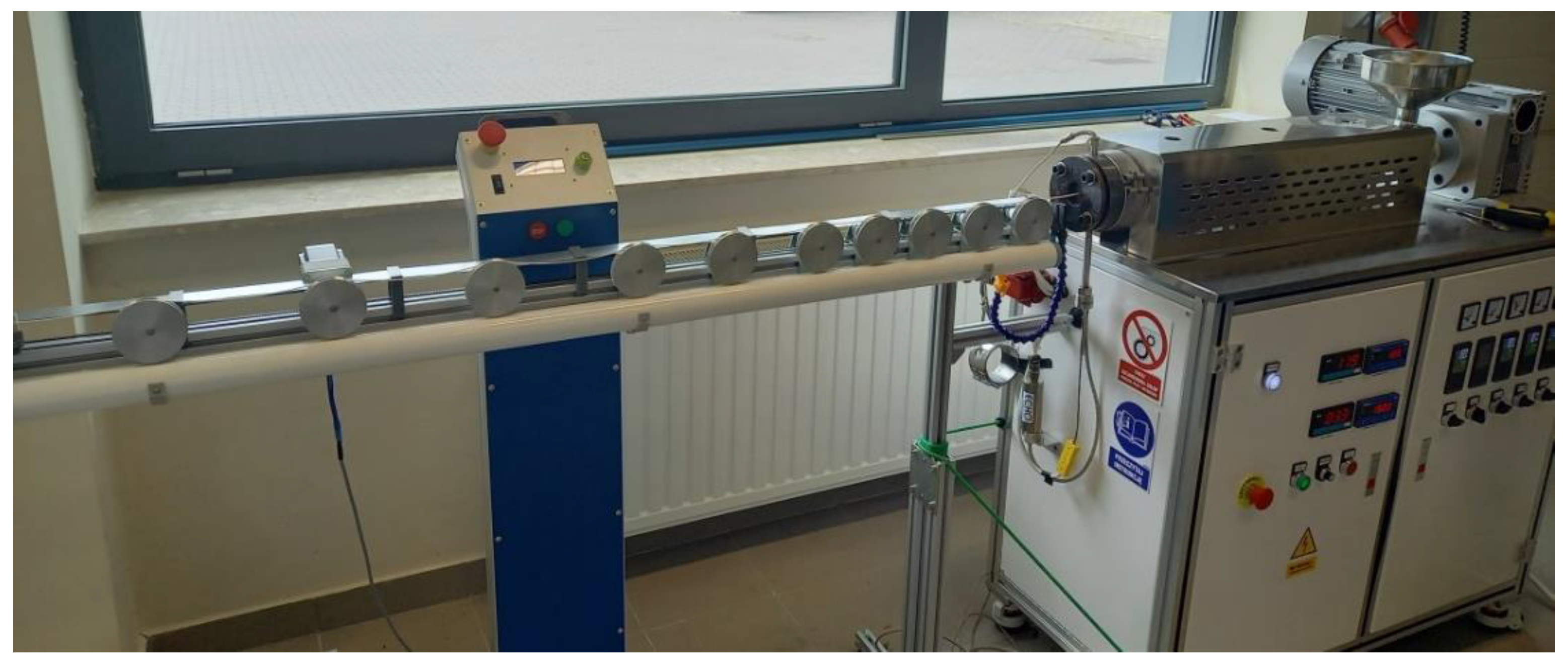
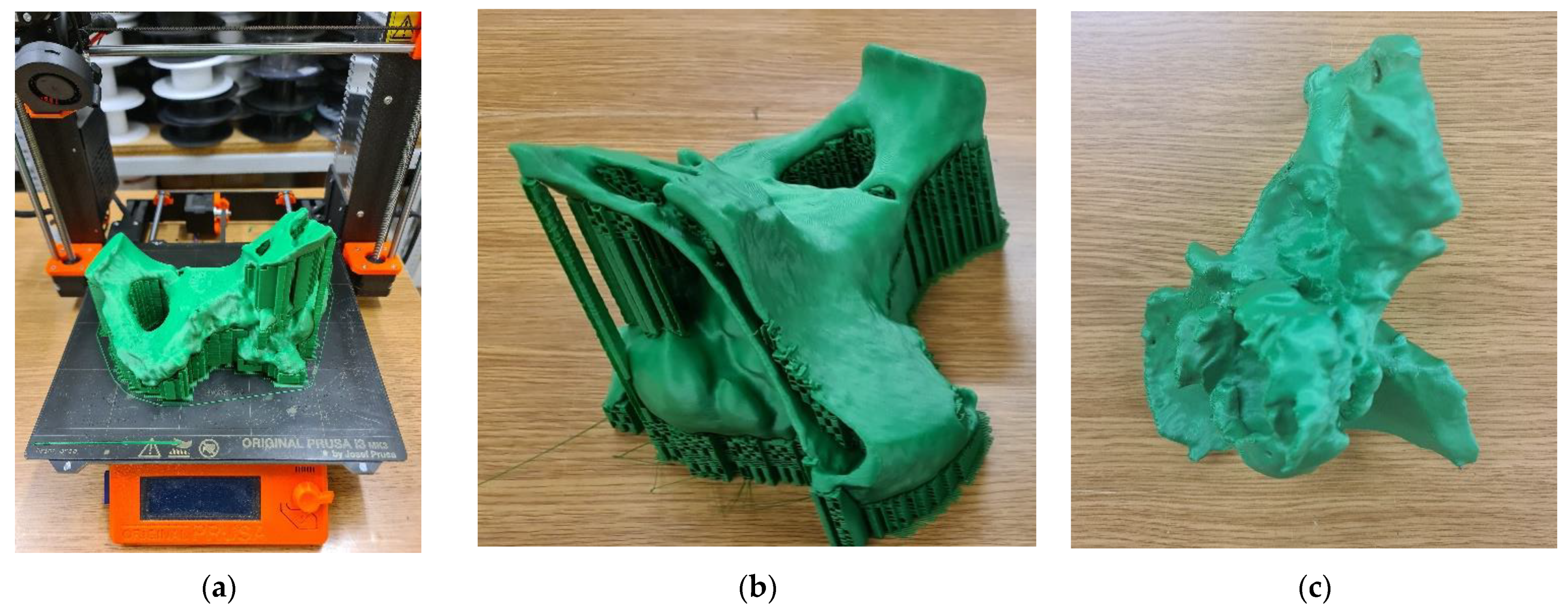
2.4. Tests of PLA-Based Polymer Materials and the Manufacturing of Anatomical Structures
3. Results
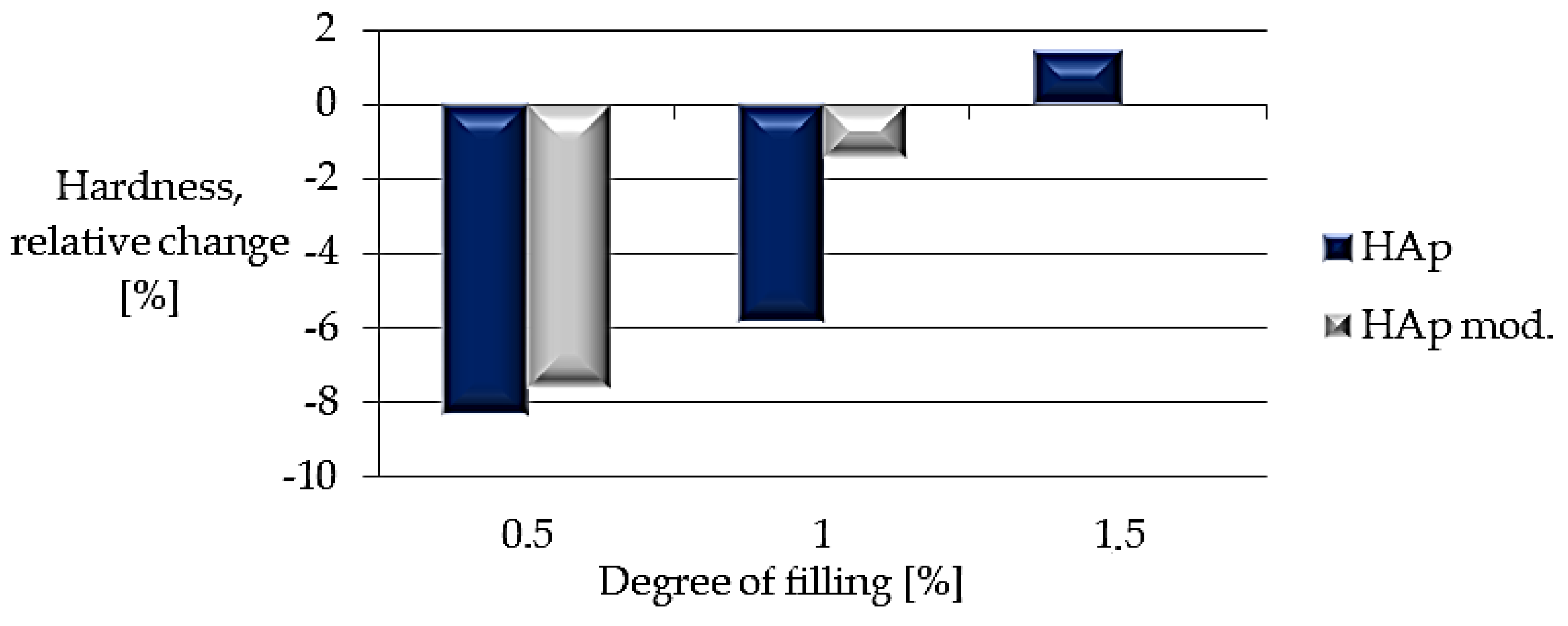
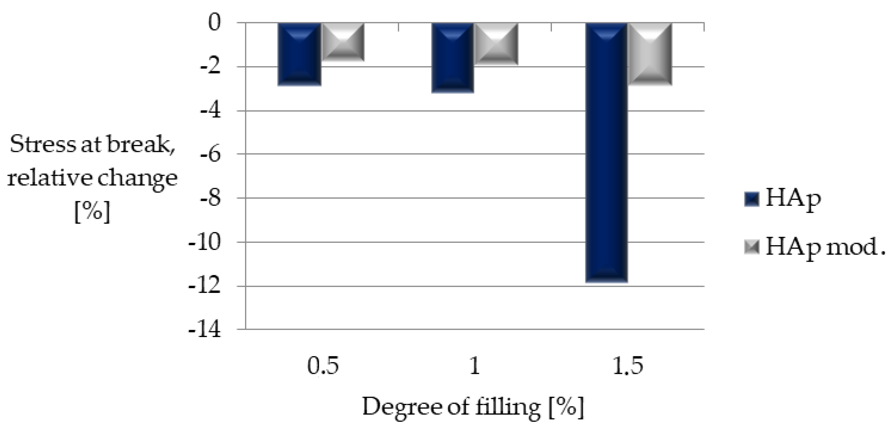
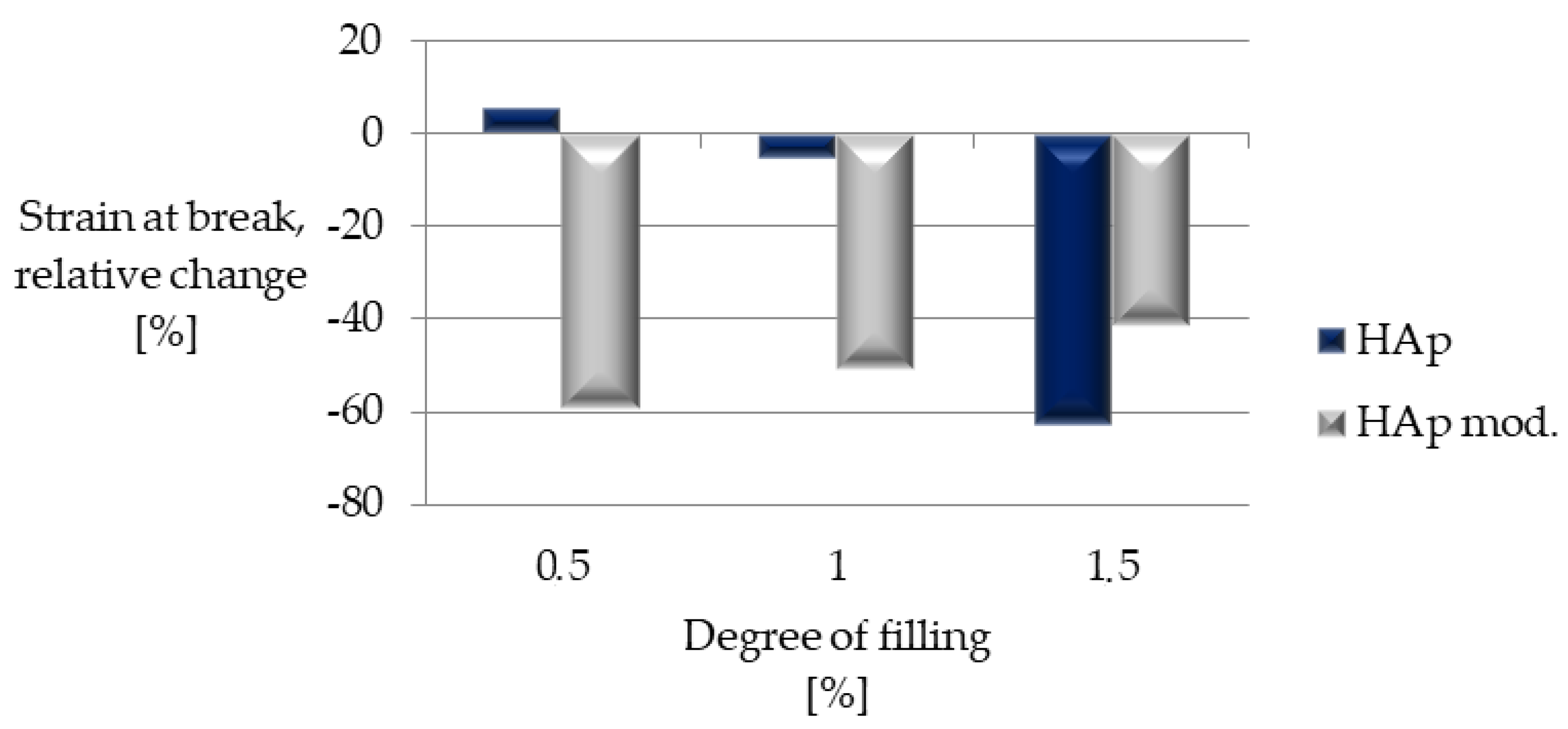
3.1. Results of Tests of PLA-Based Polymer Materials
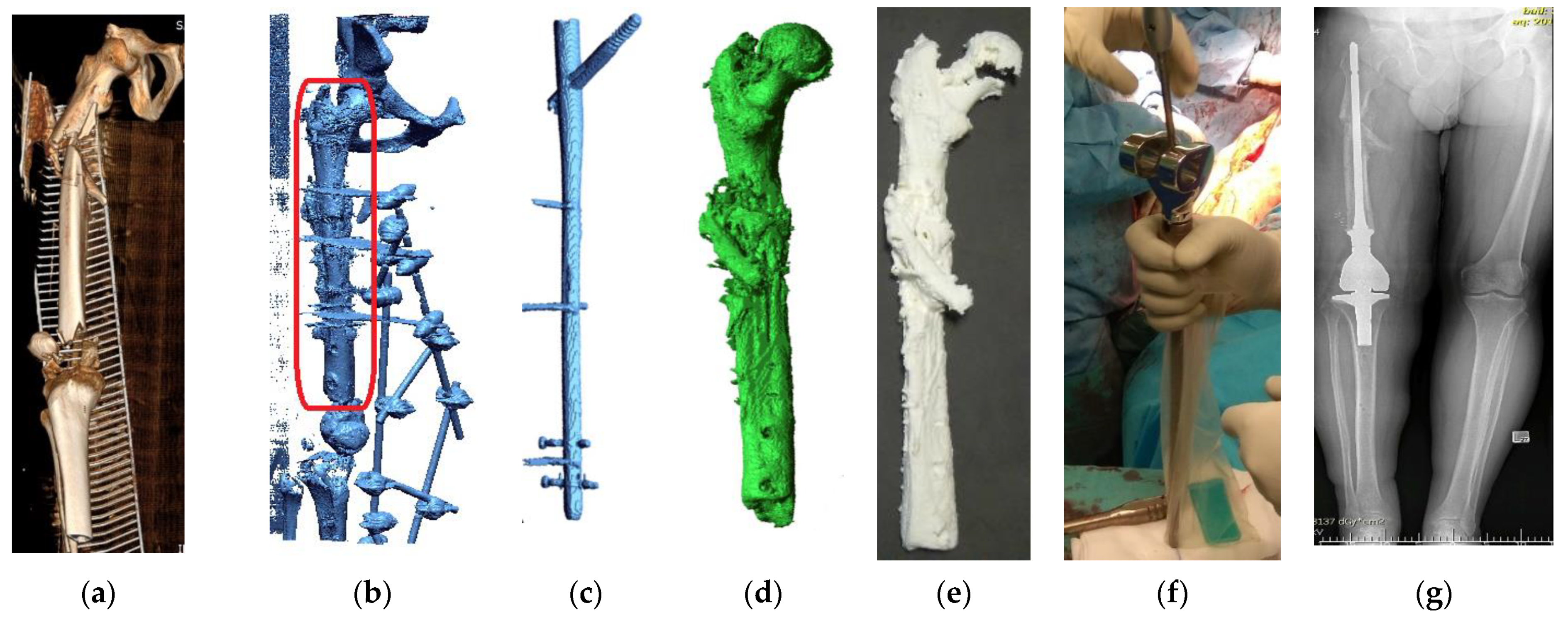
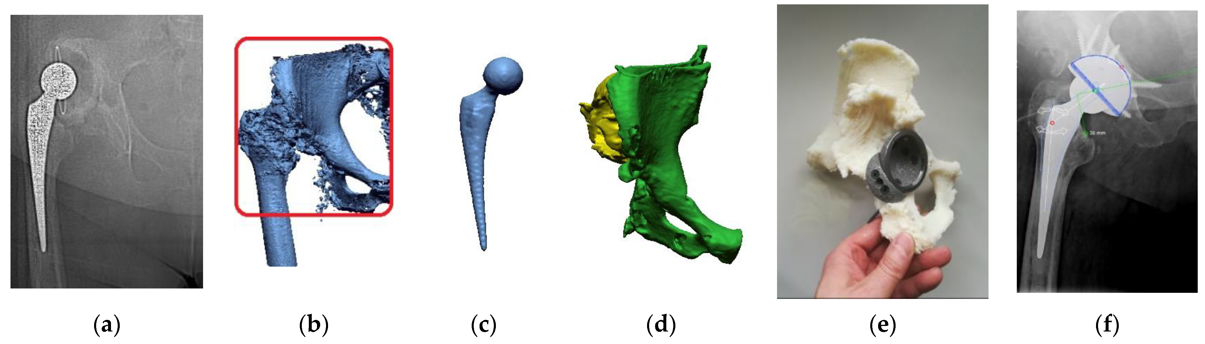
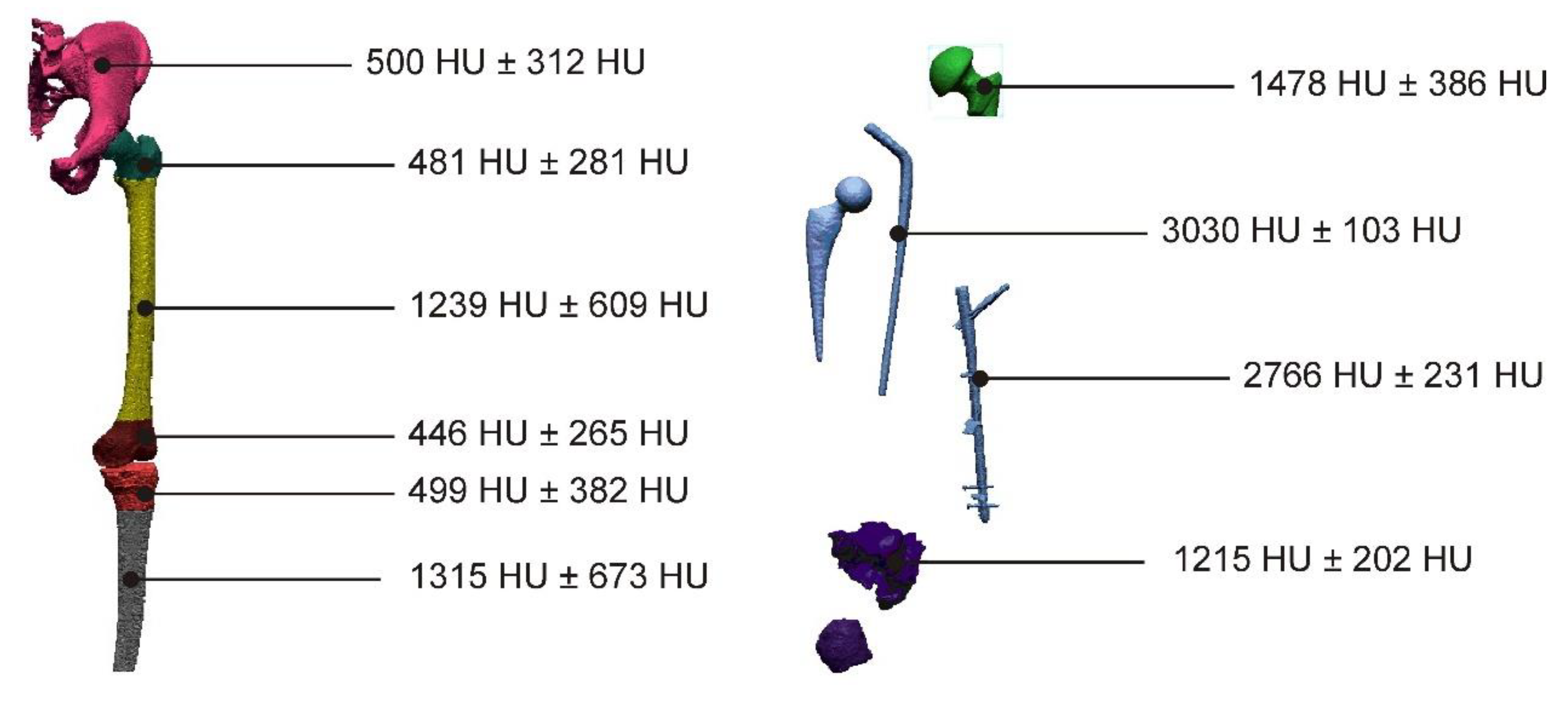
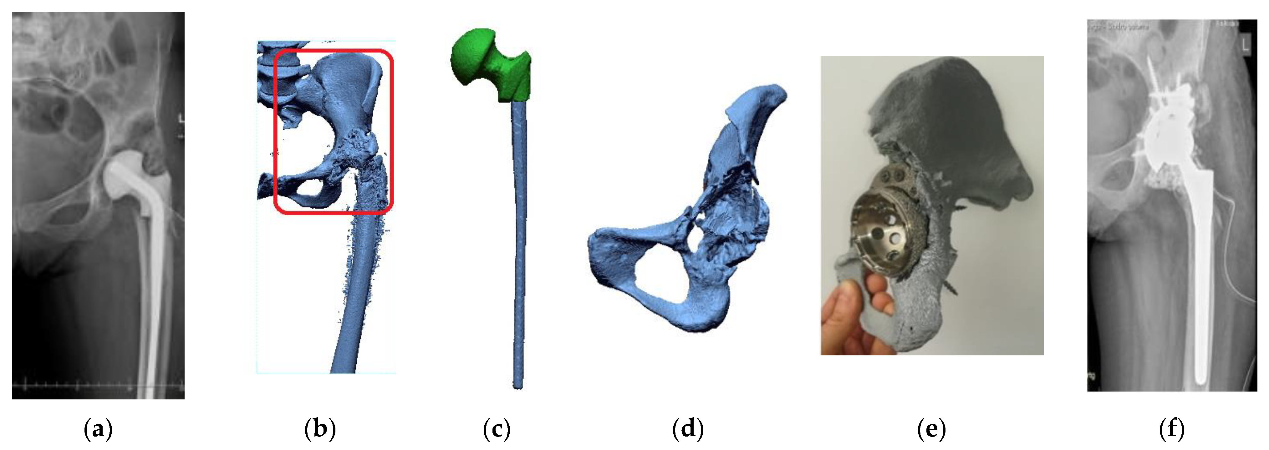
3.2. Results of Tested Procedure
4. Discussion
5. Conclusions
6. Patents
Author Contributions
Funding
Institutional Review Board Statement
Informed Consent Statement
Data Availability Statement
Acknowledgments
Conflicts of Interest
References
- Raja, V.; Kiran, J.F. Reverse Engineering—An Industrial Perspective; Springer: New York, NY, USA, 2010. [Google Scholar]
- Geng, Z.; Bidanda, B. Review of reverse engineering systems—Current state of the art. Virtual Phys. Prototyp. 2017, 12, 161–172. [Google Scholar] [CrossRef]
- Urbanic, R.J.; Elmaraghy, H.A.; Elmaraghy, W.H. A reverse engineering methodology for rotary components from point cloud data. Int. J. Adv. Manuf. Technol. 2008, 37, 1146–1167. [Google Scholar] [CrossRef]
- Baggi, E. Reverse engineering applications for recovery of broken or worn parts and re-manufacturing: Three case studies. Adv. Eng. Softw. 2009, 40, 407–418. [Google Scholar] [CrossRef]
- Bidanda, B.; Bartolo, P. (Eds.) Virtual Prototyping & Bio Manufacturing in Medical Applications; Springer: New York, NY, USA, 2008. [Google Scholar]
- Kumar, D.; Yadav, P.K.; Bhaskar, J. 3D Modelling of Human Joints Using Reverse Engineering for Biomedical Applications. In Advances in Manufacturing and Industrial Engineering; Springer: Singapore, 2021; pp. 865–875. [Google Scholar] [CrossRef]
- Budzik, G.; Turek, P.; Traciak, J. The influence of change in slice thickness on the accuracy of reconstruction of cranium geometry. Proc. Inst. Mech. Eng. Part H 2017, 231, 197–202. [Google Scholar] [CrossRef] [PubMed]
- Ford, J.M.; Decker, S.J. Computed tomography slice thickness and its effects on three-dimensional reconstruction of anatomical structures. J. Forensic Radiol. Imaging 2016, 4, 43–46. [Google Scholar] [CrossRef]
- Van Eijnatten, M.; Koivisto, J.; Karhu, K.; Forouzanfar, T.; Wolff, J. The impact of manual threshold selection in medical additive manufacturing. Int. J. Comput. Assist. Radiol. Surg. 2017, 12, 607–615. [Google Scholar] [CrossRef] [Green Version]
- Van Eijnatten, M.; van Dijk, R.; Dobbe, J.; Streekstra, G.; Koivisto, J.; Wolff, J. CT image segmentation methods for bone used in medical additive manufacturing. Med. Eng. Phys. 2018, 51, 6–16. [Google Scholar] [CrossRef]
- Preim, B.; Bartz, D. Visualization in Medicine: Theory, Algorithms, and Applications; Morgan Kaufmann: San Francisco, CA, USA, 2007. [Google Scholar]
- Romans, L. Computed Tomography for Technologists: A Comprehensive Text; Wolters Kluwer: Balitmore, MD, USA, 2011. [Google Scholar]
- Alsleem, H.; Davidson, R. Factors affecting contrast-detail performance in computed tomography: A review. J. Med. Imaging Radiat. Sci. 2013, 44, 62–70. [Google Scholar] [CrossRef]
- Vandenberghe, B.; Luchsinger, S.; Hostens, J.; Dhoore, E.; Jacob, R. The inluence of exposure parameters on jawbone model accuracy using cone beam CT and multislice CT. Dentomaxillofac. Radiol. 2014, 41, 466–474. [Google Scholar] [CrossRef] [Green Version]
- Matsiushevich, K.; Belvedere, C.; Leardini, A.; Durante, S. Quantitative comparison of freeware software for bone mesh from DICOM files. J. Biomech. 2019, 84, 247–251. [Google Scholar] [CrossRef]
- Huotilainen, E.; Jaanimets, R.; Valášek, J.; Marcián, P.; Salmi, M.; Tuomi, J.; Mäkitie, A.; Wolff, J. Inaccuracies in additive manufactured medical skull models caused by the DICOM to STL conversion process. J. Cranio Maxillofac. Surg. 2014, 42, e259–e265. [Google Scholar] [CrossRef] [PubMed]
- Van Eijnatten, M.; Berger, F.H.; De Graaf, P.; Koivisto, J.; Forouzanfar, T.; Wolff, J. Influence of CT parameters on STL model accuracy. Rapid Prototyp. J. 2017, 23, 678–685. [Google Scholar] [CrossRef]
- Gibson, I.; Rosen, D.W.; Stucker, B. Additive Manufacturing Technologies; Springer: Cham, Switzerland, 2021. [Google Scholar]
- Javaid, M.; Haleem, A. Additive manufacturing applications in medical cases: A literature based review. Alex. J. Med. 2018, 54, 411–422. [Google Scholar] [CrossRef] [Green Version]
- Tack, P.; Victor, J.; Gemmel, P.; Annemans, L. 3D-printing techniques in a medical setting: A systematic literature review. Biomed. Eng. Online 2016, 15, 115. [Google Scholar] [CrossRef] [Green Version]
- Abduo, J. Fit of CAD/CAM implant frameworks: A comprehensive review. J. Oral Implantol. 2014, 40, 758–766. [Google Scholar] [CrossRef]
- Antúnez-Conde, R.; Navarro Cuéllar, C.; Salmerón Escobar, J.I.; Díez-Montiel, A.; Navarro Cuéllar, I.; Dell’Aversana Orabona, G.; Cebrián Carretero, J.L. Intraosseous Venous Malformation of the Zygomatic Bone: Comparison between Virtual Surgical Planning and Standard Surgery with Review of the Literature. J. Clin. Med. 2021, 10, 4565. [Google Scholar] [CrossRef]
- Vanaei, H.R.; Khelladi, S.; Deligant, M.; Shirinbayan, M.; Tcharkhtchi, A. Numerical Prediction for Temperature Profile of Parts Manufactured using Fused Filament Fabrication. J. Manuf. Process. 2022, 76, 548–558. [Google Scholar] [CrossRef]
- Culmone, C.; Smit, G.; Breedveld, P. Additive manufacturing of medical instruments: A state-of-the-art review. Addit. Manuf. 2019, 27, 461–473. [Google Scholar] [CrossRef]
- Oren, D.; Dror, A.A.; Bramnik, T.; Sela, E.; Granot, I.; Srouji, S. The power of three-dimensional printing technology in functional restoration of rare maxillomandibular deformity due to genetic disorder: A case report. J. Med. Case Rep. 2021, 15, 197. [Google Scholar] [CrossRef]
- Dawood, A.; Marti, B.M.; Sauret-Jackson, V.; Darwood, A. 3D printing in dentistry. Br. Dent. J. 2015, 219, 521–529. [Google Scholar] [CrossRef]
- Gupta, H.; Bhateja, S.; Arora, G. 3D Printing and its applications in oral and maxillofacial surgery. IP J. Surg. Allied Sci. 2019, 1, 48–52. [Google Scholar]
- Schweiger, J.; Edelhoff, D.; Güth, J.-F. 3D Printing in Digital Prosthetic Dentistry: An Overview of Recent Developments in Additive Manufacturing. J. Clin. Med. 2021, 10, 2010. [Google Scholar] [CrossRef] [PubMed]
- Turek, P.; Budzik, G.; Oleksy, M.; Bulanda, K. Polymer materials used in medicine processed by additive techniques. Polimery 2020, 65, 510–515. [Google Scholar] [CrossRef]
- Eltorai, A.E.M.; Nguyen, E.; Daniels, A.H. Three-dimensional printing in orthopedic surgery. Orthopedics 2015, 38, 684–687. [Google Scholar] [CrossRef] [PubMed] [Green Version]
- Kim, J.W.; Lee, Y.; Seo, J.; Park, J.H.; Seo, Y.M.; Kim, S.S.; Shon, H.C. Clinical experience with three-dimensional printing techniques in orthopedic trauma. J. Orthop. Sci. 2018, 23, 383–388. [Google Scholar] [CrossRef]
- Moreta-Martinez, R.; Calvo-Haro, J.A.; Mediavilla-Santos, L.; Pérez-Mañanes, R.; Pascau, J. Combining Augmented Reality and 3D Printing to Improve Surgical Workflows in Orthopedic Oncology: Smartphone Application and Clinical Evaluation. Sensors 2021, 21, 1370. [Google Scholar] [CrossRef]
- Gordon, C.R. The special field of neuroplastic surgery. J. Craniofac. Surg. 2021, 32, 3–7. [Google Scholar] [CrossRef]
- Burton, H.E.; Peel, S.; Eggbeer, D. Reporting fidelity in the literature for computer aided design and additive manufacture of implants and guides. Addit. Manuf. 2018, 23, 362–373. [Google Scholar] [CrossRef]
- Lowther, M.; Louth, S.; Davey, A.; Hussain, A.; Ginestra, P.; Carter, L.; Cox, S. Clinical, industrial, and research perspectives on powder bed fusion additively manufactured metal implants. Addit. Manuf. 2019, 28, 565–584. [Google Scholar] [CrossRef] [Green Version]
- Mousavi Nejad, Z.; Zamanian, A.; Saeidifar, M.; Vanaei, H.R.; Salar Amoli, M. 3D Bioprinting of Polycaprolactone-Based Scaffolds for Pulp-Dentin Regeneration: Investigation of Physicochemical and Biological Behavior. Polymers 2021, 13, 4442. [Google Scholar] [CrossRef]
- Thévenaz, P.; Blu, T.; Unser, M. Image interpolation and resampling. Handb. Med. Imaging Process. Anal. 2000, 1, 393–420. [Google Scholar] [CrossRef]
- Lehmann, T.M.; Gonner, C.; Spitzer, K. Survey: Interpolation methods in medical image processing. IEEE Trans. Med. Imaging 1999, 18, 1049–1075. [Google Scholar] [CrossRef] [PubMed] [Green Version]
- Tsuzuki, M.D.S.G.; Sato, A.K.; Ueda, E.K.; Martins, T.D.C.; Takimoto, R.Y.; Iwao, Y.; Abe, L.I.; Gotoh, T.; Kagei, S. Propagation-based marching cubes algorithm using open boundary loop. Vis. Comput. 2018, 34, 1339–1355. [Google Scholar] [CrossRef]
- Newman, T.S.; Yi, H. A survey of the marching cubes algorithm. Comput. Graph. 2006, 30, 854–879. [Google Scholar] [CrossRef]
- Manmadhachary, A.; Kumar, R.; Krishnanand, L. Improve the accuracy, surface smoothing and material adaption in STL file for RP medical models. J. Manuf. Process. 2016, 21, 46–55. [Google Scholar] [CrossRef]
- Ledalla, S.R.K.; Tirupathi, B.; Sriram, V. Performance evaluation of various STL file mesh refining algorithms applied for FDM-RP process. J. Inst. Eng. Ser. C 2018, 99, 339–346. [Google Scholar] [CrossRef]
- Zha, W.; Anand, S. Geometric approaches to input file modification for part quality improvement in additive manufacturing. J. Manuf. Process. 2015, 20, 465–477. [Google Scholar] [CrossRef]
- Koch, F.; Thaden, O.; Tröndle, K.; Zengerle, R.; Zimmermann, S.; Koltay, P. Open-source hybrid 3D-bioprinter for simultaneous printing of thermoplastics and hydrogels. HardwareX 2021, 10, e00230. [Google Scholar] [CrossRef]
- Malik, A.; Lhachemi, H.; Ploennigs, J.; Ba, A.; Shorten, R. An application of 3D model reconstruction and augmented reality for real-time monitoring of additive manufacturing. Procedia Cirp 2019, 81, 346–351. [Google Scholar] [CrossRef]
- Wiese, M.; Thiede, S.; Herrmann, C. Rapid manufacturing of automotive polymer series parts: A systematic review of processes, materials and challenges. Addit. Manuf. 2020, 36, 101582. [Google Scholar] [CrossRef]
- Kozik, B.; Dębski, M.; Bąk, P.; Gontarz, M.; Zaborniak, M. Effect of heat treatment on the tensile properties of incrementally processed modified polylactide. Polimery 2021, 66, 357–361. [Google Scholar] [CrossRef]
- Ilyas, R.A.; Sapuan, S.M.; Harussani, M.M.; Hakimi, M.Y.A.Y.; Haziq, M.Z.M.; Atikah, M.S.N.; Asrofi, M. Polylactic acid (PLA) biocomposite: Processing, additive manufacturing and advanced applications. Polymers 2021, 13, 1326. [Google Scholar] [CrossRef] [PubMed]
- Chacón, J.M.; Caminero, M.A.; García-Plaza, E.; Núnez, P.J. Additive manufacturing of PLA structures using fused deposition modelling: Effect of process parameters on mechanical properties and their optimal selection. Mater. Des. 2017, 124, 143–157. [Google Scholar] [CrossRef]
- Sossa, P.A.F.; Giraldo, B.S.; Garcia, B.C.G.; Parra, E.R.; Arango, P.J.A. Comparative study between natural and synthetic Hydroxyapatite: Structural, morphological and bioactivity properties. Matéria 2018, 23. [Google Scholar] [CrossRef] [Green Version]
- Kula, Z.M.; Jakubowski, W.; Śmielak, B.; Szymanowski, H. Evaluation of the adhesive bonding of composite materials containing hydroxyapatite to hard dental tissues. Prosthodontics 2020, 70, 274–280. [Google Scholar] [CrossRef]
- ISO 1133-1:2011; Plastics—Determination of the Melt Mass-Flow Rate (MFR) and Melt Volume-Flow Rate (MVR) of Thermoplastics—Part 1: Standard Method. ISO: Geneva, Switzerland, 2011.
- ISO 2039-1:2001; Plastics—Determination of Hardness—Part 1: Ball Indentation Method. ISO: Geneva, Switzerland, 2001.
- ISO 179-1:2010; Plastics—Determination of Charpy Impact Properties—Part 1: Non-Instrumented Impact Test. ISO: Geneva, Switzerland, 2010.
- American Society of Mechanical Engineers (ASME). B89. 4.22. Methods for Performance Evaluation of Articulated Arm Coordinate Measuring Machines (CMM); ASME: New York, NY, USA, 2004. [Google Scholar]
- Turek, P.; Budzik, G. Estimating the Accuracy of Mandible Anatomical Models Manufactured Using Material Extrusion Methods. Polymers 2021, 13, 2271. [Google Scholar] [CrossRef]
- Turek, P.; Budzik, G.; Sęp, J.; Oleksy, M.; Józwik, J.; Przeszłowski, Ł.; Paszkiewicz, A.; Kochmański, Ł.; Zelechowski, D. An Analysis of the Casting Polymer Mold Wear Manufactured Using PolyJet Method Based on the Measurement of the Surface Topography. Polymers 2020, 12, 3029. [Google Scholar] [CrossRef]
- ISO 4288:2011; Geometrical Product Specifications (GPS)—Surface Texture: Profile Method—Rules and Procedures for the Assessment of Surface Texture. ISO: Geneva, Switzerland, 2011.
- ISO 25178-2:2012; Geometrical Product Specifications (GPS). In Surface Texture: Areal—Part 2: Terms, Definitions and Surface Texture Parameters. ISO: Geneva, Switzerland, 2012.
- Salmi, M.; Paloheimo, K.S.; Tuomi, J.; Wolff, J.; Mäkitie, A. Accuracy of medical models made by additive manufacturing (rapid manufacturing). J. Cranio-Maxillofac. Surg. 2013, 41, 603–609. [Google Scholar] [CrossRef]
- Msallem, B.; Sharma, N.; Cao, S.; Halbeisen, F.S.; Zeilhofer, H.F.; Thieringer, F.M. Evaluation of the dimensional accuracy of 3D-printed anatomical mandibular models using FFF, SLA, SLS, MJ, and BJ printing technology. J. Clin. Med. 2020, 9, 817. [Google Scholar] [CrossRef] [Green Version]
- Juneja, M.; Thakur, N.; Kumar, D.; Gupta, A.; Bajwa, B.; Jindal, P. Accuracy in dental surgical guide fabrication using different 3-D printing techniques. Addit. Manuf. 2018, 22, 243–255. [Google Scholar] [CrossRef]
- Brouwers, L.; Teutelink, A.; van Tilborg, F.A.; de Jongh, M.A.; Lansink, K.W.; Bemelman, M. Validation study of 3D-printed anatomical models using 2 PLA printers for preoperative planning in trauma surgery, a human cadaver study. Eur. J. Trauma Emerg. Surg. 2019, 45, 1013–1020. [Google Scholar] [CrossRef] [PubMed]
- Smith, M.L.; Jones, J.F. Dual-extrusion 3D printing of anatomical models for education. Anat. Sci. Educ. 2018, 11, 65–72. [Google Scholar] [CrossRef] [PubMed]
- Douraiswami, B.; Rajagopalakrishnan, R.; Sukumaran, S.A.K.; Isvaran, S. Custom Mega Prosthesis Knee: A Panacea for Intricate Trauma of Distal Femur with Bone Loss. J. Orthop. Case Rep. 2019, 9, 37–40. [Google Scholar] [CrossRef] [PubMed]
- Calori, G.M.; Colombo, M.; Ripamonti, C.; Malagoli, E.; Mazza, E.; Fadigati, P.; Bucci, M. Megaprosthesis in large bone defects: Opportunity or chimaera? Injury 2014, 45, 388–393. [Google Scholar] [CrossRef]
- Rosen, A.L.; Strauss, E. Primary Total Knee Arthroplasty for Complex Distal Femur Fractures in Elderly Patients. Clin. Orthop. Relat. Res. Number 2004, 425, 101–105. [Google Scholar] [CrossRef]
- Fleischhacker, E.; Ehrl, D.; Fürmetz, J.; Meller, R.; Böcker, W.; Zeckey, C. Rekonstruktion großer osteochondraler Defekte des distalen Femurs und der proximalen Tibia. Unfallchirurg 2021, 124, 74–79. [Google Scholar] [CrossRef]
- Rose, B.; Bartlett, W.; Blunn, G.; Briggs, T.; Cannon, S. Custom-made lateral femoral condyle replacement for traumatic bone loss: A case report. Knee 2010, 17, 417–420. [Google Scholar] [CrossRef]
- Stuyts, B.; Peersman, G.; Thienpont, E.; Van den Eeden, E.; Van der Bracht, H. Custom-made lateral femoral hemiarthroplasty for traumatic bone loss: A case report. Knee 2015, 22, 435–439. [Google Scholar] [CrossRef]
- Bulanda, K.; Oleksy, M.; Oliwa, R.; Budzik, G.; Gontarz, M. Biodegradable polymer composites based on polylactide used in selected 3D technologies. Polimery 2020, 65, 557–562. [Google Scholar] [CrossRef]
- Bari, S.S.; Chatterjee, A.; Mishra, S. Biodegradable polymer nanocomposites: An overview. Polym. Rev. 2016, 56, 287–328. [Google Scholar] [CrossRef]
- Bulanda, K.; Oleksy, M.; Oliwa, R.; Budzik, G.; Przeszłowski, Ł.; Mazurkow, A. Biodegradable polymer composites used in rapid prototyping technology by Melt Extrusion Polymers (MEP). Polimery 2020, 65, 430–436. [Google Scholar] [CrossRef]
- Kashte, S.; Jaiswal, A.K.; Kadam, S. Artificial bone via bone tissue engineering: Current scenario and challenges. Tissue Eng. Regen. Med. 2017, 14, 1–14. [Google Scholar] [CrossRef] [PubMed]
- Jariwala, S.H.; Lewis, G.S.; Bushman, Z.J.; Adair, J.H.; Donahue, H.J. 3D printing of personalized artificial bone scaffolds. 3D Print. Addit. Manuf. 2015, 2, 56–64. [Google Scholar] [CrossRef] [PubMed]


| Sample | PLA Content [%] | HAp Content [%] | HAp Mod. Content [%] |
|---|---|---|---|
| Composite I | 99.5 | 0.5 | 0.0 |
| Composite II | 99.0 | 1.0 | 0.0 |
| Composite III | 98.5 | 1.5 | 0.0 |
| Composite IV | 99.5 | 0.0 | 0.5 |
| Composite V | 99.0 | 0.0 | 1.0 |
| Composite VI | 98.5 | 0.0 | 1.5 |
| Filament Manufacturing Process | 3D-Printing Process | ||
|---|---|---|---|
| Parameters | Value | Parameters | Value |
| Temperature | 190–220 °C | Nozzle diameter | 0.4 mm |
| Screw rotational speed | 120 RPM | Layer height | 0.2 mm |
| Extraction speed | 110 mm/s | Infill percentage | 100% |
| Filament diameter | 1.75 ± 0.05 mm | Infill pattern | Rectilinear ± 45° |
| Extrusion temperature | 220 °C | ||
| Bed temperature | 40 °C | ||
| Printing speed | 70 mm/s | ||
| Parameter | Value |
|---|---|
| Preload | 1.1 kg |
| Basic load | 2.16 kg |
| Temperature | 220 °C |
| Time | 240 s |
| Sample cut-off time | 5 s |
| Sample | MFR [g/10 min] |
|---|---|
| Composite I | 24.36 ± 0.03 |
| Composite II | 24.07 ± 0.04 |
| Composite III | 27.24 ± 0.12 |
| Composite IV | 26.45 ± 0.02 |
| Composite V | 32.09 ± 0.05 |
| Composite VI | 23.64 ± 0.00 |
| PLA | 43.45 ± 0.04 |
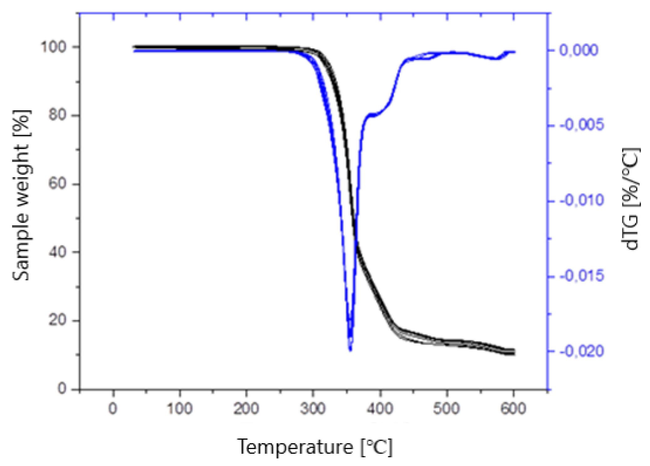
| Sample | T2% [°C] | T5% [°C] | Tmax [°C] | mmax [%] | R600 [%] |
|---|---|---|---|---|---|
| Composite I | 307.63 | 319.59 | 355.51 | 40.99 | 10.35 |
| Composite II | 312.50 | 323.97 | 355.17 | 39.13 | 10.71 |
| Composite III | 310.54 | 321.72 | 355.57 | 40.11 | 11.74 |
| Composite IV | 300.52 | 317.29 | 355.38 | 41.62 | 10.09 |
| Composite V | 306.37 | 318.12 | 354.77 | 40.67 | 11.88 |
| Composite VI | 312.99 | 324.01 | 355.39 | 38.92 | 11.77 |
| PLA | 300.69 | 315.40 | 354.17 | 43.22 | 10.18 |
| Sample | Hardness [N/mm2] |
|---|---|
| Composite I | 31.1 ± 3.9 |
| Composite II | 31.9 ± 3.9 |
| Composite III | 34.4 ± 4.0 |
| Composite IV | 31.3 ± 3.6 |
| Composite V | 33.4 ± 2.7 |
| Composite VI | 33.9 ± 4.0 |
| PLA | 33.9 ± 4.2 |
| Sample | Impact Strength [kJ/m2] |
|---|---|
| Composite I | 4.99 ± 0.57 |
| Composite II | 466 ± 0.48 |
| Composite III | 5.41 ± 1.55 |
| Composite IV | 4.17 ± 0.62 |
| Composite V | 4.25 ± 0.53 |
| Composite VI | 5.44 ± 1.16 |
| PLA | 6.62 ± 0.91 |
| Sample | Stress at Break, [MPa] | Young’s Modulus, [MPa] | Strain at Break [%] |
|---|---|---|---|
| Composite I | 32.4 ± 0.5 | 1409.0 ± 21.3 | 18.9 ± 3.8 |
| Composite II | 32.3 ± 0.5 | 1356.8 ± 24.0 | 16.9 ± 6.1 |
| Composite III | 29.4 ± 0.2 | 1275.7 ± 25.5 | 6.7 ± 4.0 |
| Composite IV | 32.7 ± 0.2 | 1376.4 ± 46.9 | 7.3 ± 4.7 |
| Composite V | 32.7 ± 0.4 | 1322.2 ± 48.1 | 8.8 ± 6.2 |
| Composite VI | 32.4 ± 1.0 | 1348.9 ± 39.3 | 10.5 ± 4.9 |
| PLA | 33.3 ± 0.8 | 1405.1 ± 54.7 | 17.9 ± 9.3 |
| Region | 3D-Printing Option | Additional 3D-Printing Parameters | Visualization | Time of 3D Printing [Days:Hours:Minutes] | Cost of 3D-Printing Model [USD] | |
|---|---|---|---|---|---|---|
| Number of Contours | Infill Percentage [%] | |||||
| Acetabulum area | Acetabulum (without added modifier)—variant 1 | 5 | 80 |  | 02:00:44 | 329.24 |
| Acetabulum (with added modifier)—variant 2 | 2 (modifier) | 15 (modifier) |  | 01:13:29 | 247.39 | |
| 5 | 80 | |||||
| Acetabulum (without added modifier)—variant 3 | 2 | 15 |  | 00:23:21 | 154.11 | |
| Bone cement (without added modifier)—variant 3 | 5 | 80 |  | 00:12:27 | 82.17 | |
| Femur bone area—upper part | Femur bone— (without added modifier)—variant 1 | 5 | 80 |  | 00:15:21 | 101.31 |
| Femur bone— (with added modifier)—variant 2 | 2 (modifier) | 15 (modifier) |  | 00:12:46 | 84.26 | |
| 5 | 80 | |||||
| Proximal femur (without added modifier)—variant 3 | 5 | 80 |  | 00:09:40 | 63.8 | |
| Femoral shaft (without added modifier)—variant 3 | 2 | 15 | 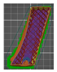 | 00:03:04 | 20.24 | |
| Femur bone area—lower part | Femur bone— (without added modifier)—variant 1 | 5 | 80 | 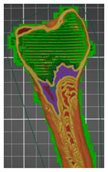 | 00:09:11 | 60.61 |
| Femur bone— (with added modifier)—variant 2 | 2 (modifier) | 15 (modifier) | 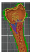 | 00:07:27 | 49.17 | |
| 5 | 80 | |||||
| Distal femur (without added modifier)—variant 3 | 5 | 80 | 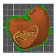 | 00:06:05 | 40.15 | |
| Femoral shaft (without added modifier)—variant 3 | 2 | 15 |  | 00:04:02 | 26.62 | |
| Tibia bone area—upper part | Tibia bone— (without added modifier)—variant 1 | 5 | 80 |  | 00:11:55 | 78.65 |
| Tibia bone— (with added modifier)—variant 2 | 2 (modifier) | 15 (modifier) |  | 00:09:24 | 62.04 | |
| 5 | 80 | |||||
| Proximal tibia (without added modifier)—variant 3 | 5 | 80 |  | 00:06:35 | 43.45 | |
| Tibia shaft (without added modifier)—variant 3 | 2 | 15 |  | 00:02:49 | 18.59 | |
| Type of Analysis | Parameters | Acetabulum | Femur Bone | Tibia Bone |
|---|---|---|---|---|
| Accuracy of geometry | Mean deviation (ӯ) [mm] | −0.012 | 0.008 | 0.020 |
| Standard deviation (σ) [mm] | 0.180 | 0.193 | 0.178 | |
| Surface roughness | Root-mean-square height (Sq) [μm] | 7.430 | 7.080 | 6.800 |
| Arithmetical mean height (Sa) [μm] | 6.020 | 5.800 | 5.930 | |
| Maximum pit height (Sv) [μm] | 14.530 | 20.750 | 16.230 | |
| Maximum peak height (Sp) [μm] | 10.540 | 9.230 | 8.320 |
| Type of Analysis | Parameters | Acetabulum Area | Femur Bone Area | Tibia Bone Area | ||||
|---|---|---|---|---|---|---|---|---|
| Acetabulum | Bone Cement | Proximal Femur | Femoral Shaft | Distal Femur | Proximal Tibia | Tibia Shaft | ||
| Accuracy of geometry | Mean deviation (ӯ) [mm] | 0.010 | 0.023 | 0.004 | −0.008 | 0.007 | 0.015 | −0.002 |
| Standard deviation (σ) [mm] | 0.124 | 0.152 | 0.102 | 0.105 | 0.162 | 0.142 | 0.092 | |
| Surface roughness | Root-mean-square height (Sq) [μm] | 5.800 | 6.020 | 5.580 | 4.380 | 5.450 | 5.920 | 5.400 |
| Arithmetical mean height (Sa) [μm] | 5.060 | 5.720 | 4.010 | 3.490 | 4.600 | 5.420 | 5.230 | |
| Maximum pit height (Sv) [μm] | 12.010 | 13.020 | 14.820 | 13.650 | 12.040 | 15.200 | 12.020 | |
| Maximum peak height (Sp) [μm] | 9.300 | 10.230 | 14.830 | 7.100 | 8.030 | 7.900 | 7.430 | |
Publisher’s Note: MDPI stays neutral with regard to jurisdictional claims in published maps and institutional affiliations. |
© 2022 by the authors. Licensee MDPI, Basel, Switzerland. This article is an open access article distributed under the terms and conditions of the Creative Commons Attribution (CC BY) license (https://creativecommons.org/licenses/by/4.0/).
Share and Cite
Turek, P.; Filip, D.; Przeszłowski, Ł.; Łazorko, A.; Budzik, G.; Snela, S.; Oleksy, M.; Jabłoński, J.; Sęp, J.; Bulanda, K.; et al. Manufacturing Polymer Model of Anatomical Structures with Increased Accuracy Using CAx and AM Systems for Planning Orthopedic Procedures. Polymers 2022, 14, 2236. https://doi.org/10.3390/polym14112236
Turek P, Filip D, Przeszłowski Ł, Łazorko A, Budzik G, Snela S, Oleksy M, Jabłoński J, Sęp J, Bulanda K, et al. Manufacturing Polymer Model of Anatomical Structures with Increased Accuracy Using CAx and AM Systems for Planning Orthopedic Procedures. Polymers. 2022; 14(11):2236. https://doi.org/10.3390/polym14112236
Chicago/Turabian StyleTurek, Paweł, Damian Filip, Łukasz Przeszłowski, Artur Łazorko, Grzegorz Budzik, Sławomir Snela, Mariusz Oleksy, Jarosław Jabłoński, Jarosław Sęp, Katarzyna Bulanda, and et al. 2022. "Manufacturing Polymer Model of Anatomical Structures with Increased Accuracy Using CAx and AM Systems for Planning Orthopedic Procedures" Polymers 14, no. 11: 2236. https://doi.org/10.3390/polym14112236
APA StyleTurek, P., Filip, D., Przeszłowski, Ł., Łazorko, A., Budzik, G., Snela, S., Oleksy, M., Jabłoński, J., Sęp, J., Bulanda, K., Wolski, S., & Paszkiewicz, A. (2022). Manufacturing Polymer Model of Anatomical Structures with Increased Accuracy Using CAx and AM Systems for Planning Orthopedic Procedures. Polymers, 14(11), 2236. https://doi.org/10.3390/polym14112236