Article

Dissolved Gases Forecasting Based on Wavelet Least Squares Support Vector Regression and Imperialist Competition Algorithm for Assessing Incipient Faults of Transformer Polymer Insulation

1
Guangxi Key Laboratory of Power System Optimization and Energy Technology, Guangxi University, Nanning 530004, Guangxi, China
2
State Grid Henan Electric Power Research Institute, Zhengzhou 450052, Henan, China
3
National Demonstration Center for Experimental Electrical Engineering Education, Guangxi University, Nanning 530004, Guangxi, China
4
Department of Electrical and Computer Engineering & Computer Science, University of New Haven, West Haven, CT 06516, USA
*
Author to whom correspondence should be addressed.
Polymers 2019, 11(1), 85; https://doi.org/10.3390/polym11010085
Submission received: 24 December 2018 / Accepted: 28 December 2018 / Published: 8 January 2019
(This article belongs to the Special Issue Polymers for Energy Applications)

Abstract

:
A solution for forecasting the dissolved gases in oil-immersed transformers has been proposed based on the wavelet technique and least squares support vector machine. In order to optimize the hyper-parameters of the constructed wavelet LS-SVM regression, the imperialist competition algorithm was then applied. In this study, the assessment of prediction performance is based on the squared correlation coefficient and mean absolute percentage error methods. According to the proposed method, this novel procedure was applied to a simulated case and the experimental results show that the dissolved gas contents could be accurately predicted using this method. Besides, the proposed approach was compared to other prediction methods such as the back propagation neural network, the radial basis function neural network, and generalized regression neural network. By comparison, it was inferred that this method is more effective than previous forecasting methods.

1. Introduction

It is generally accepted that high-quality electrical energy is at the heart of the smart grid business [1,2,3,4], and the power transformer is one of the keys to guaranteeing that the business is reliable and successful. Transformers are widely distributed in power transmission and distribution systems. Hence, the failure of power transformers is often followed by disastrous consequences, which include equipment burning and large-scale blackouts. Therefore, the reliable and stable operation of power transformer is very necessary. In order to avoid blackouts, power companies use many methods for online monitoring of transformers. Some new methods including detecting hot spot temperature, windings displacement and dissolved gas analysis (DGA), have been used to detect incipient faults in the power transformer [5]. However, dissolved gas analysis (DGA) is one of the most widely used methods [6,7,8,9]. In an oil-immersed transformer, insulating oil and oil-immersed paper are extremely important factors in the insulation ability of power transformers. The heat generated by the normal operation of the transformer cannot break the oil-hydrocarbon molecular chemical bonds of the transformer. However, when partial overheating or arc high temperature occurs, most of the heat generated by the fault will act on the insulation oil and solid insulation. The insulation material will age and generate gas at the same time. Generally, carbon monoxide (CO), carbon dioxide (CO2) hydrogen (H2), acetylene (C2H2), ethylene (C2H4), ethane (C2H6), and methane (CH4) are considered to be the seven key gases. When the transformer is overheated or discharged, it will aggravate the gas production. According to thermal degradation principles, the content of key gases is directly related to the specific fault type. A number of simple schemes such as Doernerburg, Rogers and IEC, have been employed to provide effective diagnosis by using the contents of gas compositions. The early faults in the oil-immersed transformer and their development trend can be quickly identified if the content of the gas components is predicted based on the historical data of the transformer [10,11,12].
Recently, artificial intelligence (AI) has been widely researched for its application in the field of fault analysis [13,14,15,16,17,18,19,20,21,22,23,24]. For example, some AI methods such as support vector machines (SVM), artificial neural networks and fuzzy logic inference systems have been applied to diagnose the faults in transformers. Besides, some other machine learning algorithms such as support vector regression (SVR) have been utilized to forecast the operational conditions of equipment in the future. Compared to these methods, the application of SVM in abnormal detection and fault diagnosis has marked advantages. It overcomes the local minimum, dimension, and over-fitting problems, and requires less in the scale of the training sample. As a reformulation of the standard SVM [19], the least squares support vector machine (LS-SVM) was proposed by Suykens et al. [25] Compared with the traditional quadratic programming method, applying the linear least squares criterion to the loss function can better simplify the standard SVM. Taking the simplicity and inherited advantages of SVM, including the basic principle of structural risk minimization and kernel mapping, LS-SVM can be extended to pattern recognition and regression problems [26,27,28,29,30]. The wavelet function is orthonormal in L2 (RN) space [31,32,33], however, Gaussian and polynomial kernels commonly used for SVM are not orthonormal bases. So, the wavelet function can approximate arbitrary curves in L2 (RN) space. Therefore, the simulated results show that the approximation effect of the wavelet kernel is obviously better than that of the Gaussian kernel [32,33].
In order to build wavelet LS-SVM regression (W-LSSVR), wavelet technique and LS = SVM regression were combined in this paper. By using the global optimizer imperialist competition algorithm (ICA) [34], the regularization term of W-LSSVR and the hyperparameters in kernel function were optimized by cross-validation to minimize the error objective function. These two measure criteria, squared correlation coefficient (r2) and mean absolute percentage error (MAPE) guide the performance evaluation of the proposed W-LSSVR, and represent the learning and generalization abilities of the SVM estimator [35,36]. By analyzing and comparing the experimental results, satisfactory prediction accuracy and valuable information were obtained, which highlights the significance and novelty of the proposed method.

2. Wavelet Least Squares Support Vector Machine

The nonlinear capacity of LS-SVM is tied to use of the kernel trick in pattern recognition and regression analysis, which results in mapping the input by an optimal choice of kernel function to a higher dimensional feature space. In this study, the three kinds of wavelet kernels (Morlet, Marr and DOG wavelet kernels) [6] were employed.
As for problems of regression, the model is first taken into account in the original space of the formula below:
f ( x ) = ω T φ ( x ) + β
where xRn, f(x) ∈ R, while φ(x) denotes a set of non-linear transformations. This leaves a training set {(x1, y1), …, (xl, yl)} ⊂ Rn × R, where xi is the input value and yi is the correlative objective value for sample i. The target is to conclude an assessment f(x) that approximates the actual desired y from the acceptable training samples and is as planus as possible. In the raw space, the following optimization formulation is utilized to show the LS-SVM regression:
min Φ ( ω , e ) = 1 2 ω T ω + 1 2 C i = 1 l e i 2
Subject to the equality constrains:
y i = ω T φ ( x i ) + β + e i , i = 1 , 2 , , l
Annotate ω might become potentially infinite dimensional, therefore, one cannot solve the primal optimization problem of this article that we have mentioned. Consequently, the above-mentioned optimization problem’s reformulation through a Lagrange functional into a dual optimization problem results in a method that is a function of the data, which is expressed in the primary dimensional feature space and the relevant formula is as below:
f ( x ) = i = 1 l α i K ( x , x i ) + β

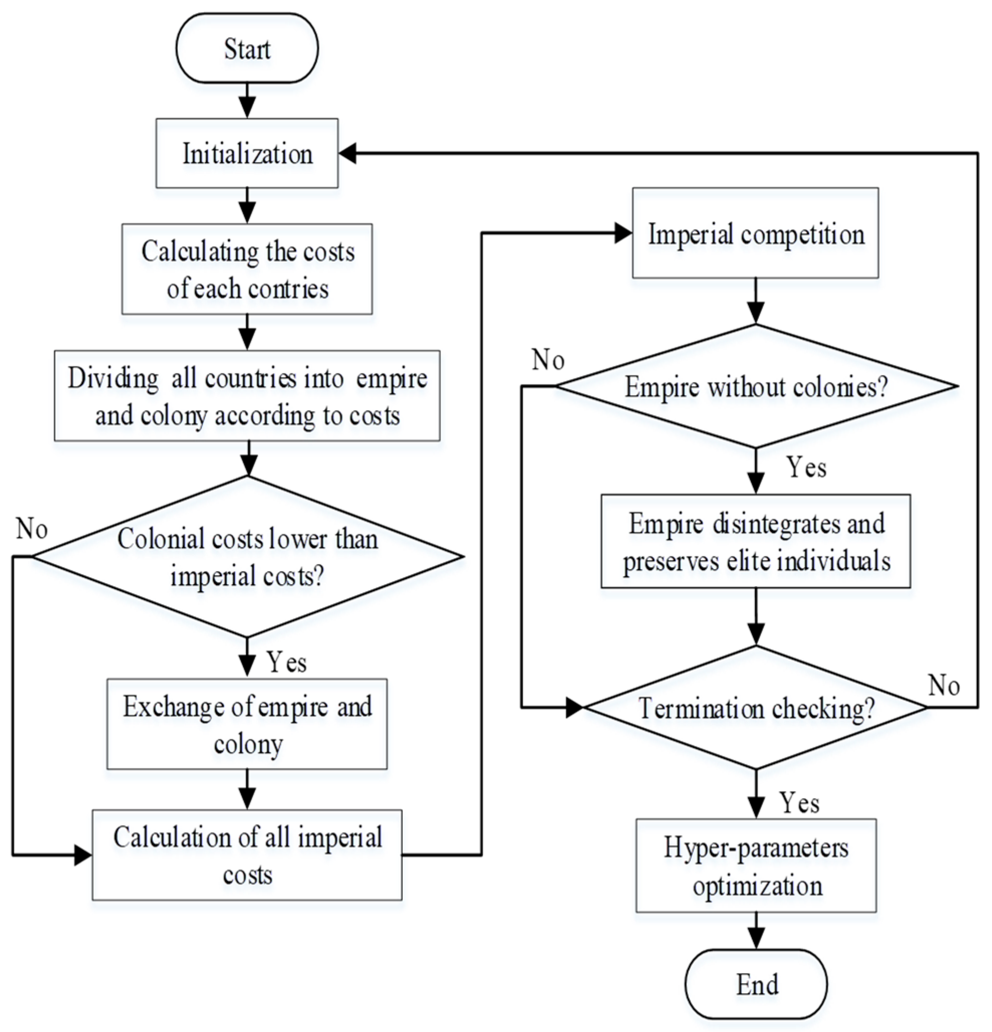
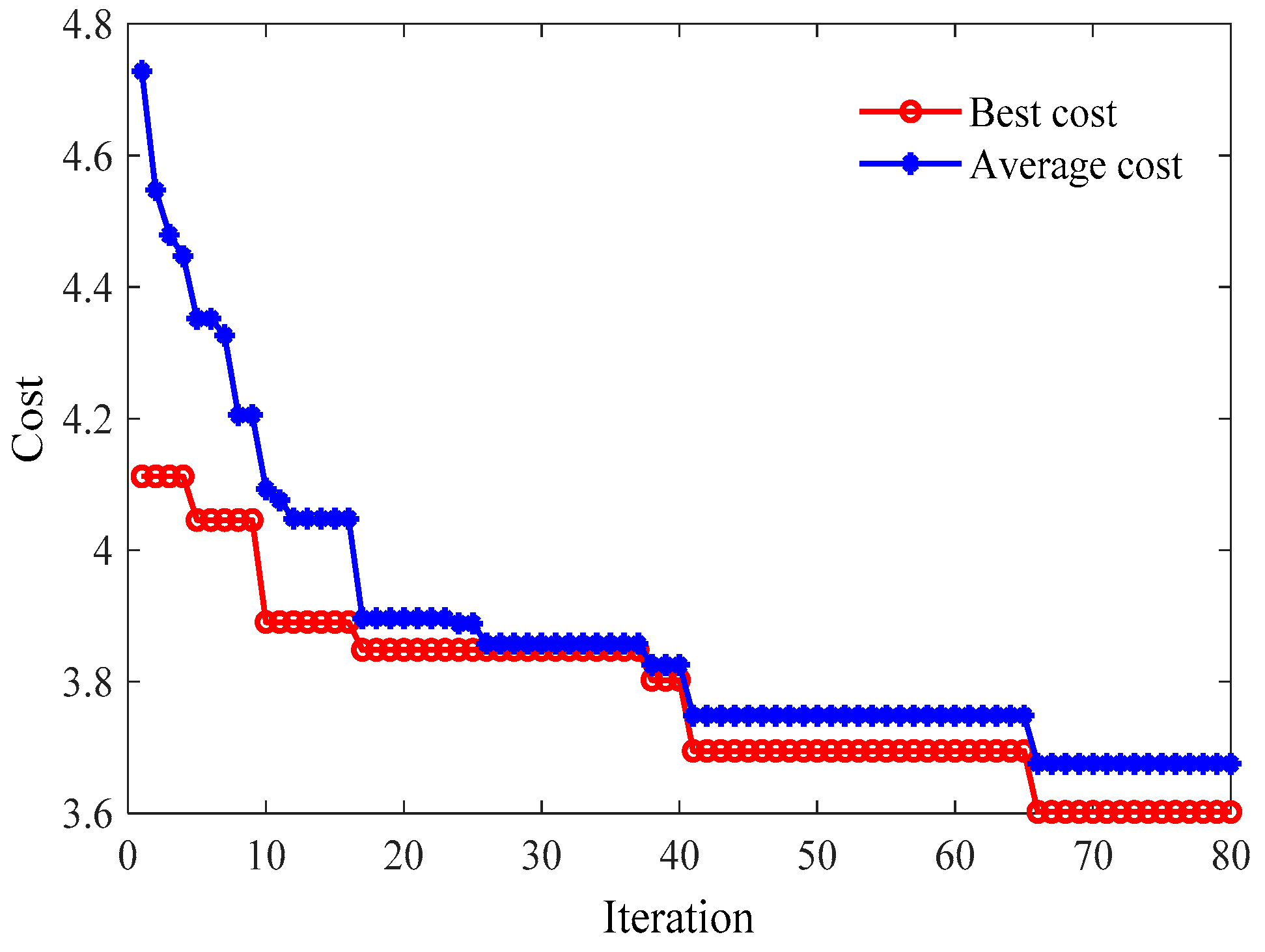
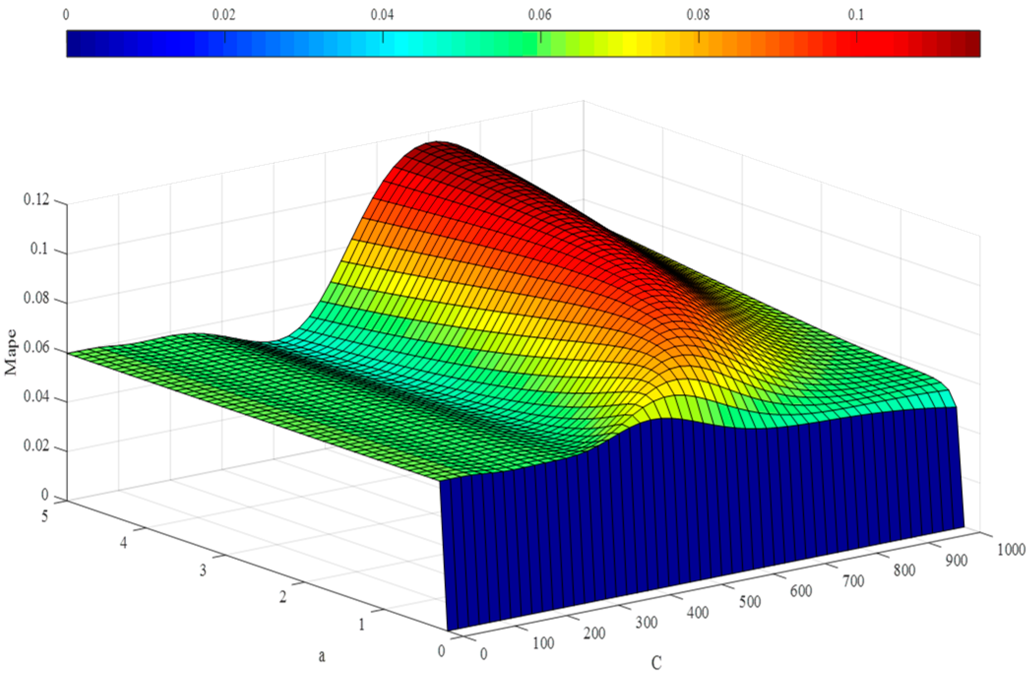
3. Using the Imperialist Competition Algorithm to Optimize Hyper-Parameters

3.1. The Imperialist Competition Algorithm

Hyper-parameters play important roles in the W-LSSVR model, thus, the selection of the hyper-parameters will affect the performance of the W-LSSVR. The main objective is to find a better way to select the optimal choices from several candidate parameters by applying cross validation. Based on this idea, it is necessary to use more rigorous approaches such as analytical techniques and heuristic algorithms to get the best hyper-parameters. While gradient-based algorithms determine the hyper-parameters of analytical techniques, modern evolutionary algorithms like simulated annealing algorithms, the genetic algorithm and imperialist competition algorithm determine the hyper-parameters of heuristic algorithms [37,38,39]. In this paper, the W-LSSVR model is optimized by using the ICA [40].
To begin with, the ICA is used to initialize the population. Then, the scope needs to be searched using some specific procedures. Eventually, this algorithm ends with the optimal solution or near optimal solution. It is noted that initial population consisted of countries—imperialists refer to the most powerful countries, colonies are the other countries. The empire is formed by both imperialists and colonies. In ICA, the initial countries are represented by the array, so the array dimension N means the number of countries N, which is defined as [p1, p2, …, pn]. The cost of the i-th country Si can be calculated by Equation (5):
S i = F ( c o u n t r y i ) = F ( P i 1 , P i 2 , P i N )
Some powerful countries (the countries with minimum cost) and Nimp countries are selected to be the imperialists from the N initial countries. At the same time, the rest of the countries are colonies belonging to the imperialists. The ICA process aims to use the minimum cost to find the most powerful country.

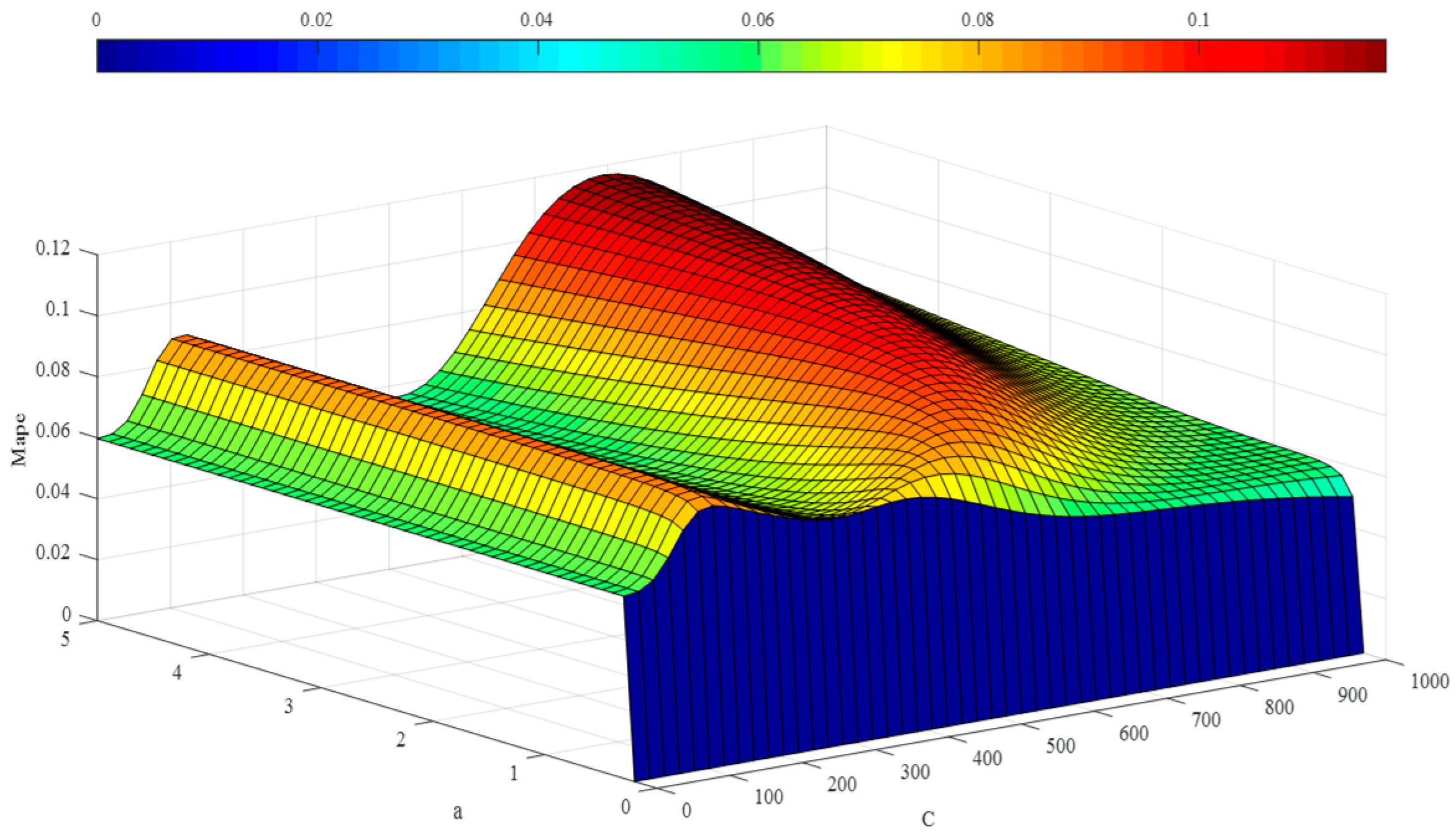
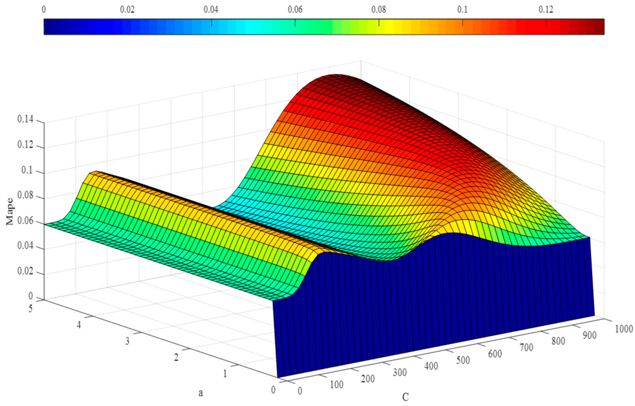
3.2. Hyper-Parameter Optimization

When optimizing the hyper-parameter with ICA, each particle stands for a potential solution, which includes the kernel parameter a and regularization parameter C. The fitness function that is relative to the optimization problem being considered is applied to measure the hyper-parameter optimality. The goal of training and testing W-LSSVR is to minimize the errors between the actual values and the forecasting values of the testing samples, which can enhance the generalization performance of the regression model. Thus, the fitness function is shown as follows:
F i t n e s s = 1 k i = 1 k 1 m j = 1 m ( f ( x i j ) y i j ) 2
where k is the number of folds in cross validation, m is the number of each subset as validation, yij is the true value, and f(xij) is the forecasting value of the validation samples.
According to the goal of minimizing the fitness function, the particle with the minimal fitness value should be reserved during the optimization process since it outperforms the other particles. Consequently, it is able to choose the optimal hyper-parameters.
The process of ICA for hyper-parameter optimization is presented in the following steps:
Step 1: Initialize parameters of ICA and set up fitness function model.
Step2: Divide all countries into two kinds, imperialists and colonies according to their costs. The countries with higher cost are empires while the countries with lower costs are colonies.
Step 3: If the colonial costs are lower than the imperial costs, exchange the empire and colony, if not, loop to the next step.
Step4: Use a differential evolution arithmetic operator and calculate the total cost of the empires.
Step5: Implement the competition of the imperialists.
Step 6: If there is an empire without any colonies, disintegrate the empires and preserve elite individuals.
Step7: When the selected condition is satisfied, the flow meets the termination condition. In this case, end the algorithm and get the optimal parameters. Repeat this process from step 1 if it does not meet the termination condition. The termination condition is defined below:
(1)
The location of the united empire is the expected solution to the optimal problem because the unique empire controls all empires and colonies.
(2)
Reaching the maximum generations.
Figure 1 shows the flowchart of ICA for hyper-parameter optimization:

4. Procedure for Forecasting Key Gas Contents with Wavelet Least Squares Support Vector Machine Regression and Imperialist Competition Algorithm

The various stages, which are based on the above-mentioned W-LSSVR and ICA processes are explained as follows. All the wavelet techniques and LS-SVM algorithms in this study were coded in MATLAB.
Stage 1: Data preprocessing
A collection of original data can be obtained from the crucial gas contents. After extracting the raw data, the training and testing sets can be generated separately. Since it is only possible to get the raw sample data from the power company on an irregular basis, the primary sampling data needs to be changed into an equal interval time series by means of interpolation methods—as can be seen, the Hermite spline interpolation [41] is used in this study. Finally, the raw data is normalized, which includes training and testing data, and which enhances the generalization ability of W-LSSVR.
Stage 2: Implement ICA to optimize hyper-parameters
In the optimizing process, cross validation is applied to ICA. The k-fold cross validation divides the training data into k disjunct sets when the training data is once substituted randomly. In the i-th (i = 1, 2, …, k) iteration, the performance of the model trained on the other k − 1 set (called training set) can be estimated by the i-th set (called the validation set). In the end, the mean value is used to get k different performance estimates.
Stage 3: Training and testing
With the optimal hyper-parameters obtained from ICA implementation, the W-LSSVR training model based upon the training data can be built, and the outputs based on the testing data will be forecasted.
It is possible to establish the W-LSSVR training model with the training data by using the optimal hyper-parameters determined from ICA implementation. Then, the output of the testing data is predicted.
In order to verify the performance in the training stages, the squared correlation coefficient (called r2) and mean absolute percentage error (MAPE) are used as evaluation indicators. However, in the testing stage, only MAPE is used as the evaluation indictor. Assuming x1, …, xl are the training data and f(x1), …, f(xl) are the predicting values by W-LSSVR. In addition, assuming y1, …, yl, are the true values, then, the r2 and MAPE can be defined as follows:
r 2 = ( l i = 1 l f ( x i ) y i i = 1 l f ( x i ) i = 1 l y i ) 2 ( l i = 1 l f ( x i ) 2 ( i = 1 l f ( x i ) ) 2 ) ( l i = 1 l y i 2 ( i = 1 l y i ) 2 )
MAPE = 1 l i = 1 l | f ( x i ) y i y i |

5. Results and Comparisons

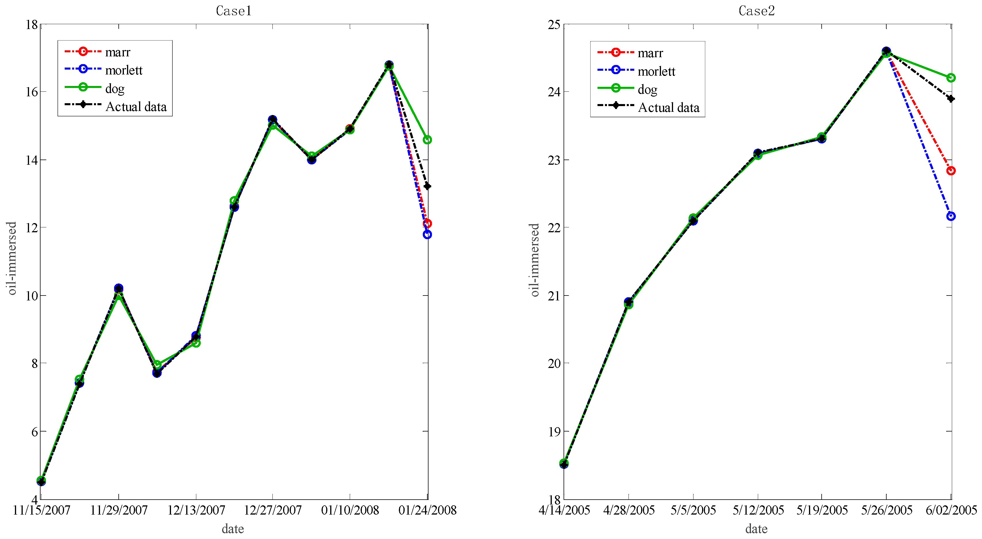
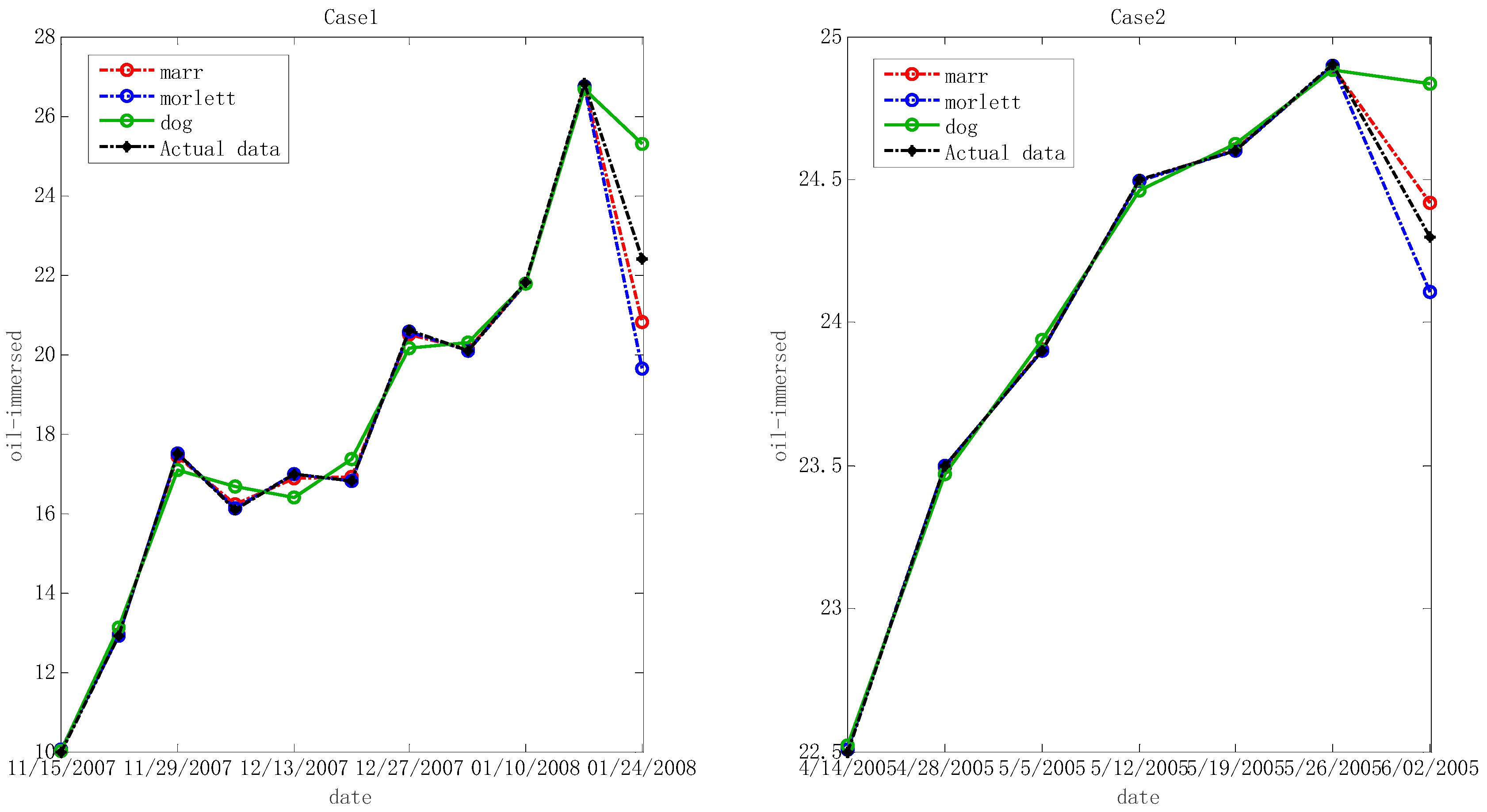
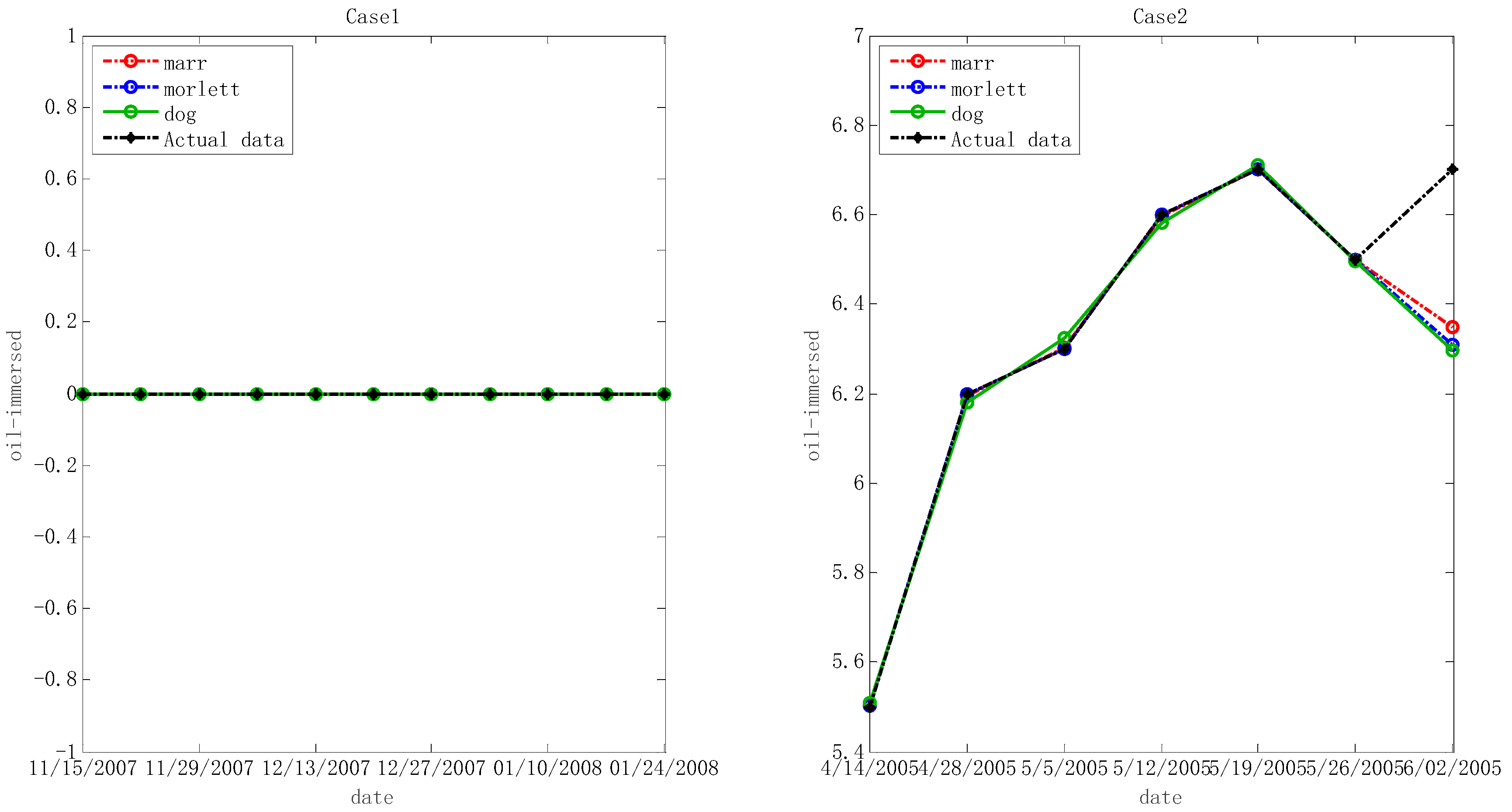
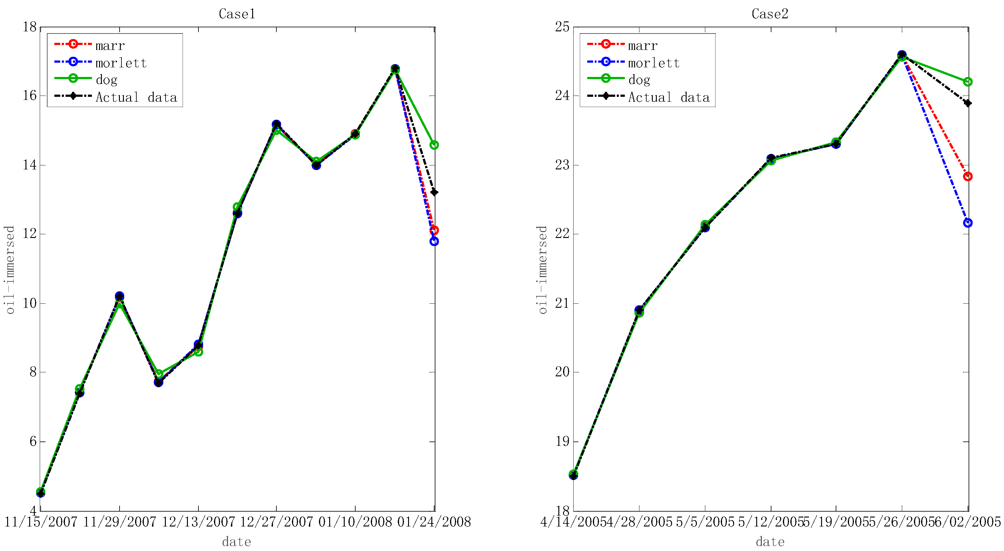
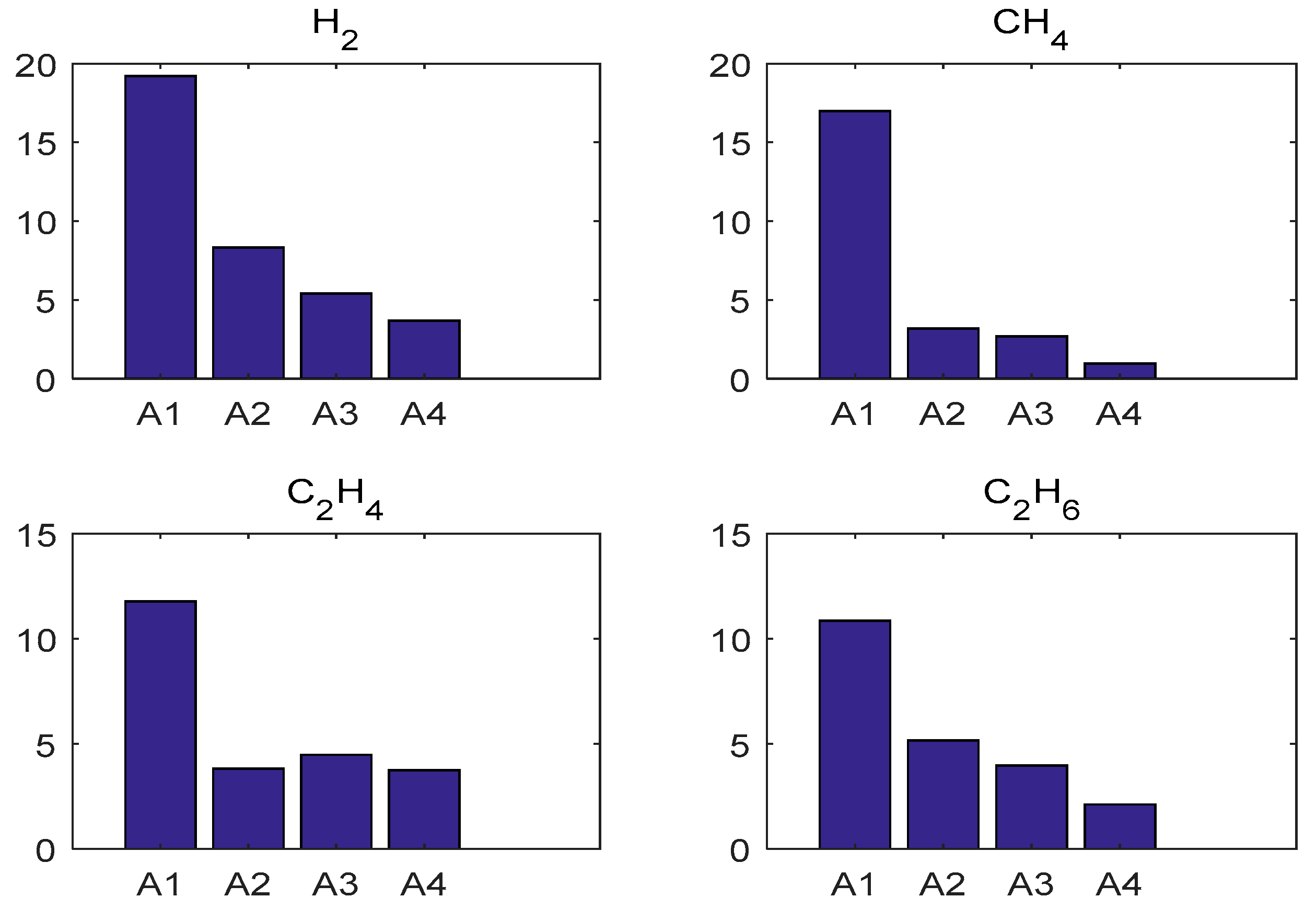
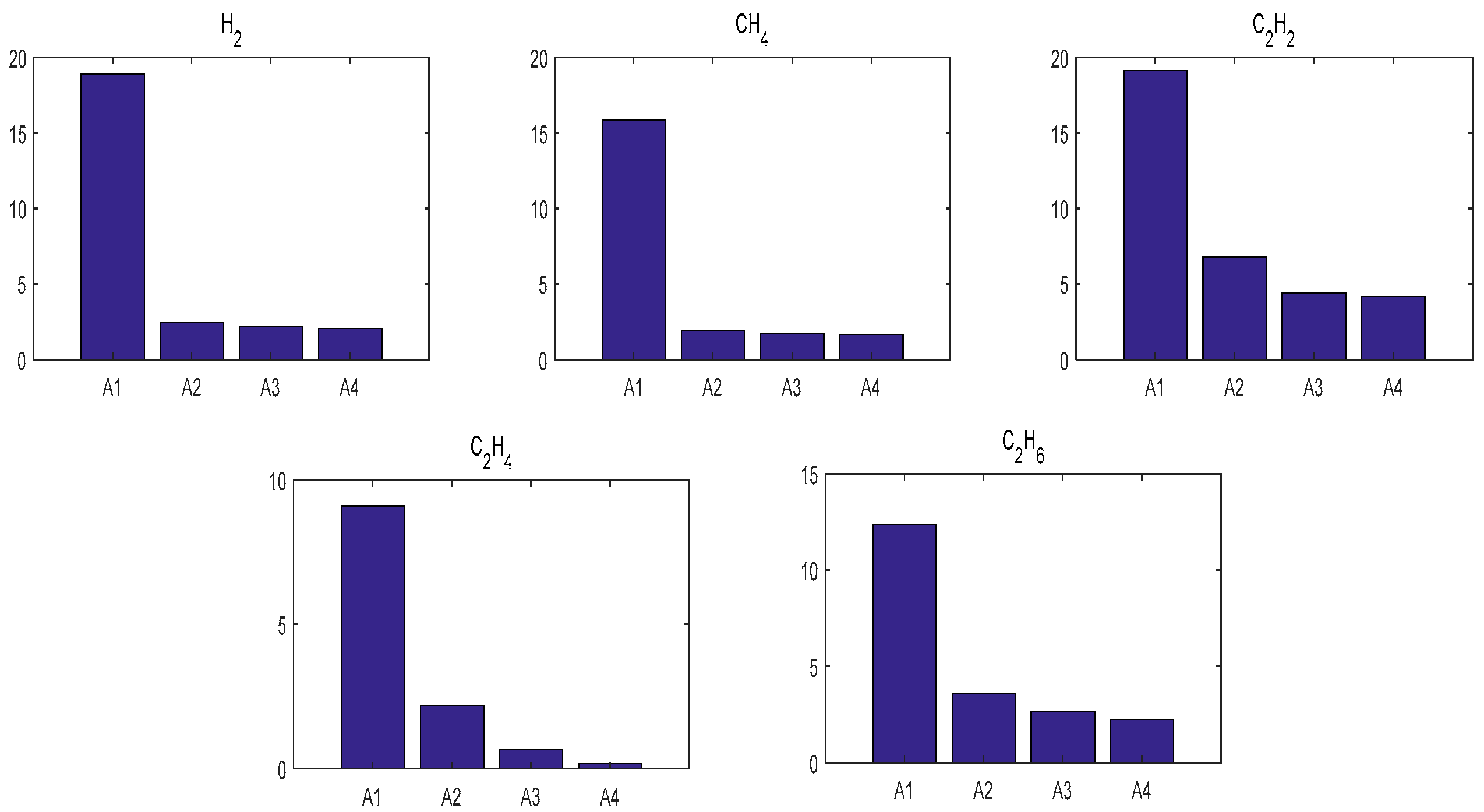
5.1. Experimental Results Based upon Wavelet Least Squares Support Vector Machine Regression and the Imperialist Competition Algorithm

The dissolved gas data collected from several Chinese power companies in [6] are used as the key gas content data for oil-immersed transformers (H2, CH4, C2H2, C2H4 and C2H6) to demonstrate the effectiveness of the proposed forecasting model. The rating of the tested transformers is 110 kV.
In the study, the aforementioned three kinds of wavelet kernels including Morlet, Marr and DOG are investigated. For Case 1, the periodical sampling time was the period between November 2009 and January 2010. First, the experimental data, including training data and testing data were normalized before applying W-LSSVR. Then, taking the Morlet W-LSSVR as an example, the algorithm of ICA with mutation is implanted to find the optimal hyper-parameters for each group of the key gas contents by using 5-fold cross validation. The parameters of the ICA algorithm used in this paper are as follows: the number of countries and the number of initial imperialists were fixed to 20 and 6, respectively; the dimension of the optimized function was set to 2; the maximum number of generations was 100; the revolution rate was set to 0.3; the assimilation coefficient equaled 2, and the assimilation angle coefficient equaled 0.5.
Figure 2 shows the convergence process of ICA with Morlet W-LSSVR for C2H4. In Figure 2, the ordinate of the coordinates represents the cost of the empire, which is negatively correlated with fitness of the candidate solution, and the abscissa represents the iterations of ICA. It can be seen from Figure 2 that the both the “Best cost” and “Average cost” curves decrease during the iteration, which means the best fitness and the average fitness of empires are increased after iterations. In other words, the W-LSSVR can obtain more appropriate values for hyper-parameters as well as better performance after being optimized by ICA.
In the step below, the optimal hyper-parameters are utilized to train Morlet, Marr and DOG W-LSSVR separately. The MAPE and r2 are proposed to measure the performance of the prediction model. The accuracy of the predicted outcome is examined by using the testing data. Morlet, Marr and DOG were respectively used as the wavelet kernel of W-LSSVR to predict in Case 1 and Case 2. The prediction results for the five gases are shown in the Figure 3, Figure 4, Figure 5, Figure 6 and Figure 7. It can be seen from Figure 3, Figure 4, Figure 5, Figure 6 and Figure 7 that the three kinds of W-LSSVR exhibit a favorable prediction performance as the prediction curves are almost identical to the curve of the actual value. Furthermore, the prediction curves of W-LSSVR with Morlet, Marr and DOG for five gases in Case 1 and Case 2 are almost coincident, therefore, the performance of W-LSSVR with any of the above three as the wavelet kernel is not very different. Figure 8, Figure 9 and Figure 10 illustrate the relationship between C, a, and the MAPE by using three kernel functions, respectively. The X-axis, Y-axis, and Z-axis represent C, a and MAPE, individually. Owing to the fact that Morlet, Marr and DOG W-LSSVR belong to the identical wavelet family and have some similar characteristics, the distinction between the performances is not that clear.
Table 1 shows the prediction performance and the optimal hyper-parameters of Morlet, Marr and DOG W-LSSVR. It can be seen from Table 1 that “Marr” wins the “top 1” seven times, followed by the “DOG” with two times. Furthermore, the “Marr” never ranked at the bottom, while the “Morlet” and “DOG” did so four and five times, respectively. According to the overall comparison of all gas prediction, the “Marr” is regarded as the most appropriate wavelet kennel for the W-LSSVR model and was adopted in our study.

5.2. Comparisons

Various forecasting models based on BPNN, SVR and PSO-W-LSSVR were performed in the same training and testing conditions for the purpose of comparison. It was necessary to normalize all the experimental data before training. Morlet W-LSSVR was chosen as an example to test and verify the forecasting accuracy. In the BPNN model, the most excellent network model for BPNN can be found by a hidden-layer network with the transfer function of log-sigmoid by training the BPNN 30 times to choose the best networks. Thus, the BPNN is generated by a hidden layer of 30 neurons and five input and output nodes. The training of BPNN takes the Levenberg Marquardt optimization method into account to minimize the expected default error value with the fastest speed.
Table 2 illustrates the evaluation performances of BPNN, SVR, PSO-W-LSSVR and ICA-W-LSSVR in MAPE and r2. By analyzing Table 2, it can be seen that the learning ability of ICA-W-LSSVR during the training stage was excellent—its training error was less than 1% and its r2 close to 1. When comparing the data of the testing stage, it shows that the MAPE of ICA-W-LSSVR is less than 4%, which is much smaller than that of BPNN, SVR and PSO-W-LSSVR. The MAPE results for the four forecasting approaches for gases in the two Cases are shown in Figure 11 and Figure 12. As shown in Figure 11 and Figure 12, the W-LSSVR has a significantly better performance than the other three approaches. It can be inferred that W-LSSVR based on ICA has better prediction accuracy and generalization performance than the other methods.

6. Conclusions

In this paper, a novel method that can be used to predict dissolved gases in transformers by combining wavelet technology with LS-SVM is proposed. Test results showed that the proposed method is feasible—a high-precision prediction model for oil-dissolved gases in transformers has been established. The method effectively evaluates the transformer condition. Besides, the forecasting results were able to provide valuable information for the arrangement of maintenance schemes. There are several points to summarize this study, which are shown below:
  • In theory, arbitrary curves can be approximated in L2 (RN) space by the wavelet function that is known as a set of bases. Therefore, the wavelet technique is combined with LS-SVM to find a new forecasting method in this study. The results of the analysis infer that the admissible wavelet kernels, including Morlet, Marr and DOG wavelet kernels exist.
  • Simply, only two parameters need to be chosen in W-LSSVR as compared to the standard SVM regression. Moreover, the optimal hyper-parameters are available by applying the imperialist competition algorithm.
  • In many cases, the given forecasting procedure is effective to predict the useful gas contents in oil-dissolved transformers. The ICA based W-LSSVR has outstanding predicting ability for actual limited samples, and this is better than that of SVR, PSO-W-LSSVR and BPNN.
It is noted that this new method takes the fault diagnosis method into account to provide more useful information for future fault analysis of transformer polymer insulation. Therefore, a follow-up study needs to investigate this further.

Author Contributions

J.L., H.Z. and Y.Z. designed the algorithms and performed the writing, H.Z. and Y.Z. are both corresponding authors and they contributed equally to this work; X.L., J.F., Y.L. and C.L. analyzed the data; Y.L. and J.Z. contributed the literature search, discussion and paper modification; all authors have approved the submitted manuscript.

Acknowledgments

The authors acknowledge the National Natural Science Foundation of China (61364027; 61473272; 51867003), the Natural Science Foundation of Guangxi (2018JJB160056; 2018JJB160064; 2018JJA160176) in their support of this work.

Conflicts of Interest

All the authors declare no conflict of interest.

References

  1. Li, J.S.; Zhou, H.W.; Meng, J.; Yang, Q.; Chen, B. Carbon emissions and their drivers for a typical urban economy from multiple perspectives: A case analysis for Beijing city. Appl. Energy 2018, 226, 1076–1086. [Google Scholar] [CrossRef]
  2. Liu, J.; Zheng, H.; Zhang, Y.; Wei, H.; Liao, R. Grey Relational Analysis for Insulation Condition Assessment of Power Transformers Based Upon Conventional Dielectric Response Measurement. Energies 2017, 10, 1526. [Google Scholar] [CrossRef]
  3. Zhang, Y.; Liu, J.; Zheng, H.; Wei, H.; Liao, R. Study on quantitative correlations between the ageing condition of transformer cellulose insulation and the large time constant obtained from the extended Debye model. Energies 2017, 10, 1842. [Google Scholar] [CrossRef]
  4. Liu, J.; Zheng, H.; Zhang, Y.; Zhou, T.; Zhao, J.; Li, J.; Liu, J.; Li, J. Comparative Investigation on the Performance of Modified System Poles and Traditional System Poles Obtained from PDC Data for Diagnosing the Ageing Condition of Transformer Polymer Insulation Materials. Polymers 2018, 10, 191. [Google Scholar] [CrossRef]
  5. Zhang, Y.; Wei, H.; Yang, Y.; Zheng, H.; Zhou, T.; Jiao, J. Forecasting of Dissolved Gases in Oil-immersed Transformers Based upon Wavelet LS-SVM Regression and PSO with Mutation ☆. Energy Procedia 2016, 104, 38–43. [Google Scholar] [CrossRef]
  6. Zheng, H.; Zhang, Y.; Liu, J.; Wei, H.; Zhao, J.; Liao, R. A novel model based on wavelet LS-SVM integrated improved PSO algorithm for forecasting of dissolved gas contents in power transformers. Electr. Power Syst. Res. 2018, 155, 196–205. [Google Scholar] [CrossRef]
  7. Tang, H.; Goulermas, J.Y.; Wu, H.; Richardson, Z.J.; Fitch, J. A probabilistic classifier for transformer dissolved gas analysis with a particle swarm optimizer. IEEE Trans. Power Del. 2008, 23, 751–759. [Google Scholar]
  8. Chatterjee, A.; Bhattacharjee, P.; Roy, N.K.; Kumbhakar, P. Usage of nanotechnology based gas sensor for health assessment and maintenance of transformers by DGA method. Int. J. Electr. Power Energy Syst. 2012, 45, 137–141. [Google Scholar] [CrossRef]
  9. Chatterjee, A.; Roy, N.K. Health monitoring of power transformers by dissolved gas analysis using regression method and study the effect of filtration on oil. World Acad. Sci. Eng. Technol. 2009, 59, 37–42. [Google Scholar]
  10. IEEE. IEEE Guide for the Interpretation of Gases Generated in Oil-Immersed Transformers; IEEE Std. C57; IEEE: Piscataway, NJ, USA, 2008. [Google Scholar]
  11. Duval, M.; Depablo, A. Interpretation of gas-in-oil analysis using new IEC publication 60599 and IEC TC 10 databases. IEEE Elect. Insul. Mag. 2001, 17, 31–41. [Google Scholar] [CrossRef]
  12. Wang, M. Grey-extension method for incipient fault forecasting of oil-immersed power transformer. Electr. Power Compon. Syst. 2004, 32, 959–975. [Google Scholar] [CrossRef]
  13. Hippert, H.S.; Pedreira, C.E.; Souza, R.C. Neural networks for short-term load forecasting: A review and evaluation. IEEE Trans. Power Syst. 2001, 16, 44–55. [Google Scholar] [CrossRef]
  14. Chang, F.; Chen, Y. Estuary water-stage forecasting by using radial basis function neural network. J. Hydrol. 2003, 270, 158–166. [Google Scholar] [CrossRef]
  15. Leung, M.T.; Chen, A.; Daouk, H. Forecasting exchange rates using general regression neural networks. Comput. Oper. Res. 2000, 27, 1093–1110. [Google Scholar] [CrossRef]
  16. Wang, M.; Hung, C. Novel grey model for the prediction of trend of dissolved gases in oil-filled power apparatus. Electr. Power Syst. Res. 2003, 67, 53–58. [Google Scholar] [CrossRef]
  17. Fei, S.; Sun, Y. Forecasting dissolved gases content in power transformer oil based on support vector machine with genetic algorithm. Electr. Power Syst. Res. 2008, 78, 507–514. [Google Scholar] [CrossRef]
  18. Li, Y.; Tong, S.; Li, T. Adaptive fuzzy output feedback control for a single-link flexible robot manipulator driven DC motor via backstepping. Nonlinear Anal. Real. 2013, 14, 483–494. [Google Scholar] [CrossRef]
  19. Vapnik, V.N. The Nature of Statistical Learning Theory. Technometrics 1997, 38, 409. [Google Scholar]
  20. Ganyun, L.V.; Cheng, H.; Zhai, H.; Dong, L. Fault diagnosis of power transformer based on multi-layer SVM classifier. Electr. Power Syst. Res. 2005, 75, 9–15. [Google Scholar] [CrossRef]
  21. Jardine, A.K.S.; Lin, D.; Banjevic, D. A review on machinery diagnostics and prognostics implementing condition-based maintenance. Mech. Syst. Signal Process. 2006, 20, 1483–1510. [Google Scholar] [CrossRef]
  22. Si, X.S.; Wangbde, W.; Zhouc, D.H. Remaining useful life estimation—A review on the statistical data driven approaches. Eur. J. Oper. Res. 2011, 213, 1–14. [Google Scholar] [CrossRef]
  23. Benmoussa, S.; Djeziri, M.A.; Benmoussa, S.; Djeziri, M.A.; Benmoussa, S.; Djeziri, M.A. Remaining useful life estimation without needing for prior knowledge of the degradation features. Iet Sci. Meas. Techno. 2017, 11, 1071–1078. [Google Scholar] [CrossRef]
  24. Djeziri, M.A.; Benmoussa, S.; Sanchez, R. Hybrid method for remaining useful life prediction in wind turbine systems. Renew. Energy 2017, 116, 173–187. [Google Scholar] [CrossRef]
  25. Suykens, J.A.K.; Gestel, T.V.; Brabanter, J.D.; Moor, B.D.; Vandewalle, J. Least Squares Support Vector Machines. Int. J. Circ. Theor. Appl. 2015, 27, 605–615. [Google Scholar] [CrossRef]
  26. Van Gestel, T.; Suykens, J.K.; Baestaens, D.E.; Lambrechts, A.; Lanckriet, G.; Vandaele, B.; Moor, D.B.; Vandewalle, J. Financial time series prediction using least squares support vector machines within the evidence framework. IEEE Trans. Neural Networ. 2001, 12, 809–821. [Google Scholar] [CrossRef] [PubMed] [Green Version]
  27. De Kruif, B.J.; De Vries, T.J.A. Pruning error minimization in least squares support vector machines. IEEE Trans. Neural Netw. 2003, 14, 696–702. [Google Scholar] [CrossRef] [PubMed] [Green Version]
  28. Gestel, T.V.; Suykens, J.A.K.; Baesens, B.; Viaene, S.; Vanthienen, J.; Dedene, G.; Moor, D.B.; Vandewalle, J. Benchmarking least squares support vector machine classifiers. Neural Process. Lett. 1999, 9, 293–300. [Google Scholar] [CrossRef]
  29. Zhang, Y.; Liu, Y. Traffic forecasting using least squares support vector machines. Transportmetrica 2009, 5, 193–213. [Google Scholar] [CrossRef]
  30. Yang, Z.; Gu, X.; Liang, X.; Ling, L. Genetic algorithm-least squares support vector regression based predicting and optimizing model on carbon fiber composite integrated conductivity. Mater. Des. 2010, 31, 1042–1049. [Google Scholar] [CrossRef]
  31. Zhang, Q.; Benveniste, A. Wavelet networks. IEEE Trans. Neural Netw. 1992, 3, 889–898. [Google Scholar] [CrossRef]
  32. Zhang, L.; Zhou, W.; Jiao, L. Wavelet support vector machine. IEEE Trans. Syst. Man Cybern. Part B Cybern. 2004, 34, 34–39. [Google Scholar] [CrossRef]
  33. Wu, Q. The forecasting model based on wavelet v-support vector machine. Expert Syst. Appl. 2009, 36, 7604–7610. [Google Scholar] [CrossRef]
  34. Kaveh, A.; Talatahari, S. Optimum design of skeletal structures using imperialist competitive algorithm. Comput. Struct. 2010, 88, 1220–1229. [Google Scholar] [CrossRef]
  35. Chang, C.; Lin, C. LIBSVM—A Library for Support Vector Machines. Available online: http://www.csie.ntu.edu.tw/~cjlin/libsvm (accessed on 1 January 2011).
  36. Smola, A.J.; Schölkopf, B.; Müller, K.R. The connection between regularization operators and support vector kernels. Neural Netw. 1998, 11, 637–649. [Google Scholar] [CrossRef] [Green Version]
  37. Hadji, M.M.; Vahidi, B.A. Solution to the Unit Commitment Problem Using Imperialistic Competition Algorithm. IEEE Trans. Power Syst. 2012, 27, 117–124. [Google Scholar] [CrossRef]
  38. Liang, J.; Qin, A.; Suganthan, P.N.; Baskar, S. Comprehensive learning particle swarm optimizer for global optimization of multimodal functions. IEEE Trans. Evol. Comput. 2006, 10, 281–295. [Google Scholar] [CrossRef]
  39. Talatahari, S.; Azar, B.F.; Sheikholeslami, R. Imperialist competitive algorithm combined with chaos for global optimization. Commun. Nonlinear Sci. 2012, 17, 1312–1319. [Google Scholar] [CrossRef]
  40. Atashpaz-Gargari, E.; Lucas, C. Imperialist competitive algorithm: An algorithm for optimization inspired by imperialistic competition. In Proceedings of the IEEE Congress on Evolutionary Computation, Singapore, 25–28 September 2007; pp. 4661–4667. [Google Scholar]
  41. Duan, Q.; Li, S.; Bao, F.; Twizell, E.H. Hermite interpolation by piecewise rational surface. Appl. Math. Comput. 2008, 198, 59–72. [Google Scholar]
Figure 1. Flowchart of hyper-parameter optimization by using ICA.
Polymers 11 00085 g001
Figure 2. Convergence curves of ICA with Morlet W-LSSVR for C2H4 in Case 1.
Polymers 11 00085 g002
Figure 3. Forecasting results with three kinds of W-LSSVRs for C2H6 in Case 1 and Case 2.
Polymers 11 00085 g003
Figure 4. Forecasting results with three kinds of W-LSSVRs for C2H4 in Case 1 and Case 2.
Polymers 11 00085 g004
Figure 5. Forecasting results with three kinds of W-LSSVRs for C2H2 in Case 1 and Case 2.
Polymers 11 00085 g005
Figure 6. Forecasting results with three kinds of W-LSSVRs for CH4 in Case 1 and Case 2.
Polymers 11 00085 g006
Figure 7. Forecasting results with three kinds of W-LSSVRs for H2 in Case 1 and Case 2.
Polymers 11 00085 g007
Figure 8. The relationship between C, a, and the MAPE of Morlet W-LSSVR for C2H4 in Case 1.
Polymers 11 00085 g008
Figure 9. The relationship between C, a, and the MAPE of Marr W-LSSVR for C2H4 in Case 1.
Polymers 11 00085 g009
Figure 10. The relationship between C, a, and the MAPE of DOG W-LSSVR for C2H4 in Case 1.
Polymers 11 00085 g010
Figure 11. Testing MAPE results of the five forecasting approaches for gases in Case 1. (A1: BPNN, A2: SVR, A3: PSO-W-LSSVR, A4: ICA-W-LSSVR).
Polymers 11 00085 g011
Figure 12. Testing MAPE results of the five forecasting approaches for gases in Case 2. (A1: BPNN, A2: SVR, A3: PSO-W-LSSVR, A4: ICA-W-LSSVR).
Polymers 11 00085 g012
Table 1. The optimal parameters and prediction performance of Morlet, Marr and DOG W-LSSVR (◆: Morlet, ●: Marr, ■: DOG).
Case No.GasKernelHyper-ParametersTestingRanking
(1/2/3)
CaMAPE (%)
1H2Morlet968.8347104.0601◇◇◆
Marr563.84976.71853.6785●○○
DOG394.77116.41143.9803□■□
CH4Morlet822.76347.59231.1321◇◆◇
Marr837.94211.47130.9675●○○
DOG995.82782.03431.3872□□■
C2H4Morlet210.9271.88283.9879◇◆◇
Marr251.57362.84533.7385●○○
DOG766.46367.83394.4210□□■
C2H6Morlet985.82786.56172.6413◇◇◆
Marr961.63983.76562.1140●○○
DOG995.89981.99112.3002□■□
2H2Morlet768.75478.99792.5740◇◇◆
Marr833.87585.89302.0665○●○
DOG394.77735.88301.8542■□□
CH4Morlet452.73167.88901.8003◇◆◇
Marr797.88512.07541.6653●○○
DOG989.42991.89971.9899□□■
C2H2Morlet517.87604.88774.3780◇◆◇
Marr457.00418.55424.1681●○○
DOG486.11289.04115.2119□□■
C2H4Morlet687.99042.00620.1949◇◆◇
Marr774.88312.78310.1684●○○
DOG882.11397.55720.2120□□■
C2H6Morlet456.14367.00322.4780◇◇◆
Marr946.44323.66452.2409○●○
DOG890.33232.32101.9930■□□
Table 2. The evaluation performances of BPNN, RBFNN, GRNN and W-LSSVR in MAPE and r2.
Case No.GasTrainingTesting
MAPE (%)r2MAPE (%)
BPNNSVRPSO-W-LSSVRICA-W-LSSVRBPNNSVRPSO-W-LSSVRICA-W-LSSVRBPNNSVRPSO-W-LSSVRICA-W-LSSVR
1H214.98347.24560.19620.24460.71870.91680.99990.999919.20118.32485.42383.6785
CH413.56122.62970.54990.55790.74790.9680.99970.999516.983.1982.68320.9675
C2H2////////////
C2H49.99122.32160.35370.49320.81090.99990.99980.999511.78013.82274.47613.7385
C2H610.54123.28840.189912.1130.83220.94850.99990.892510.86115.15413.96062.114
2H216.14761.12920.48721.20390.76320.9760.99990.978718.91872.46282.15672.0665
CH414.01210.83250.30710.31120.810.98150.99990.985915.86011.91071.75431.6653
C2H218.18903.46730.51940.88780.75110.9710.99980.917819.12226.77954.3854.1681
C2H48.98320.52310.08710.970.85320.97850.99990.93039.10112.19420.67410.1684
C2H611.98671.34530.51840.43660.77650.96260.99980.962212.39013.6092.65212.2409

