Simultaneous Prediction of the Magnetic and Crystal Structure of Materials Using a Genetic Algorithm


Abstract
:1. Introduction
2. Materials and Methods
2.1. Materials Modelling
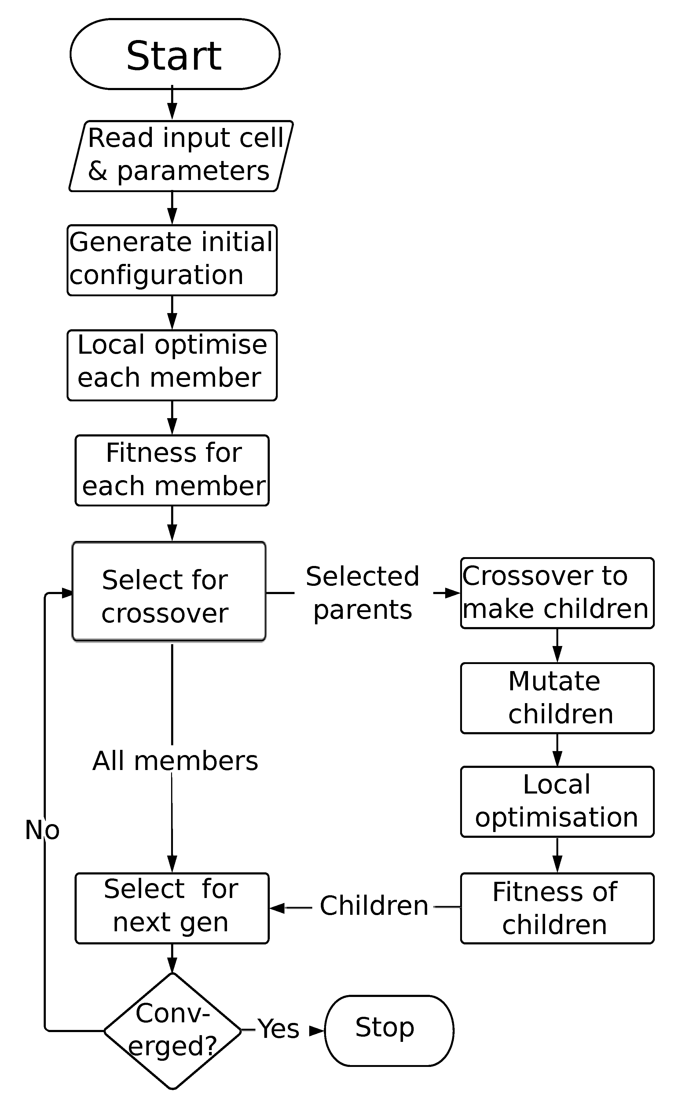
2.2. Genetic Algorithms
2.3. Extending the GA for Magnetic Materials
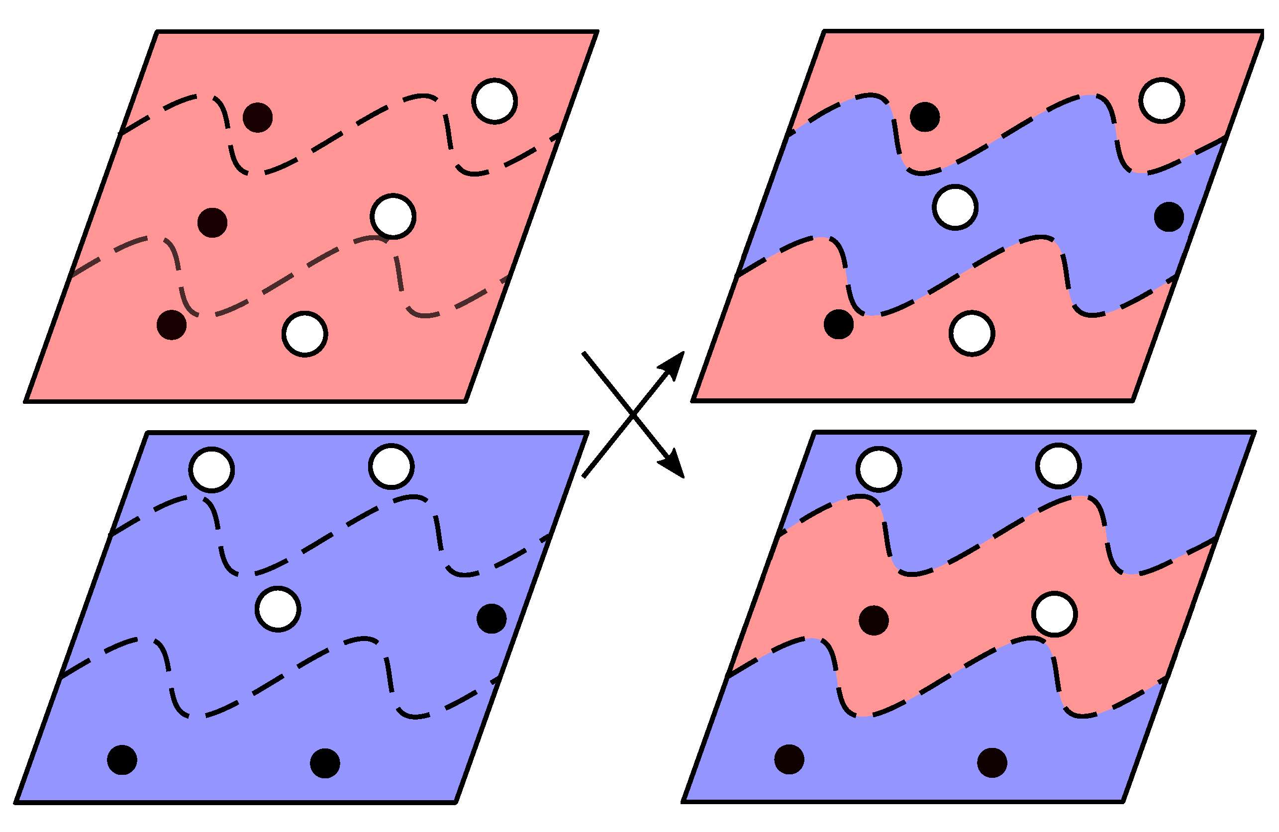
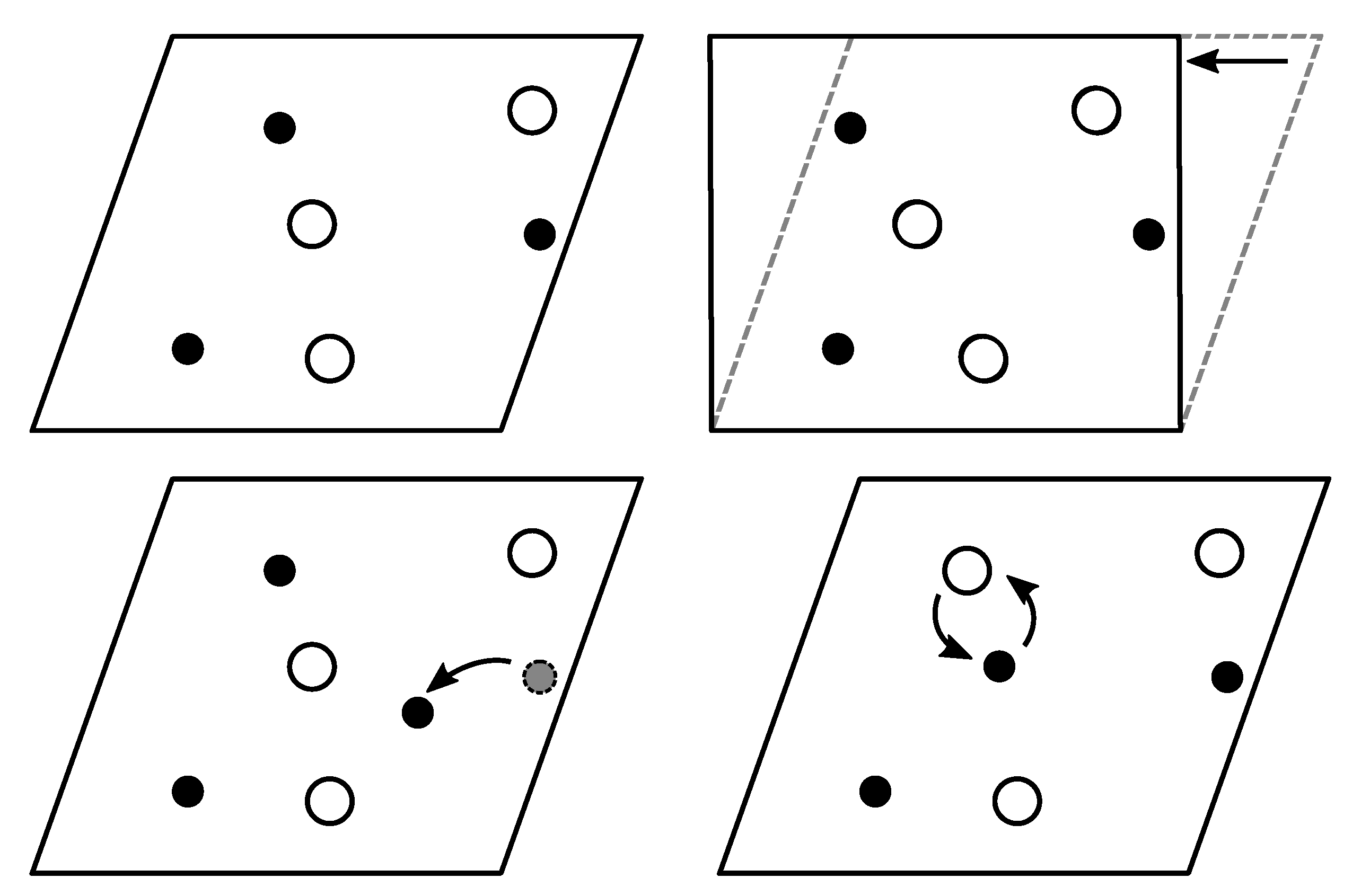
2.3.1. Perturbation/Permutation Operations
2.3.2. Magnetic Fingerprinting
2.4. Case Studies
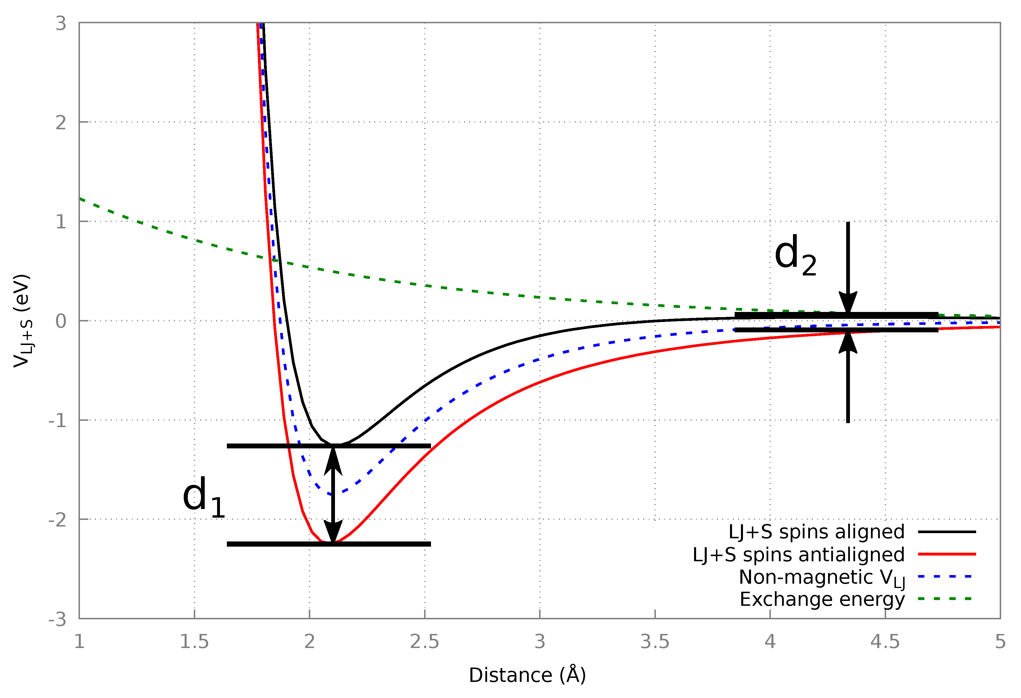
2.4.1. Fictional Magnetic Potential: LJ + S
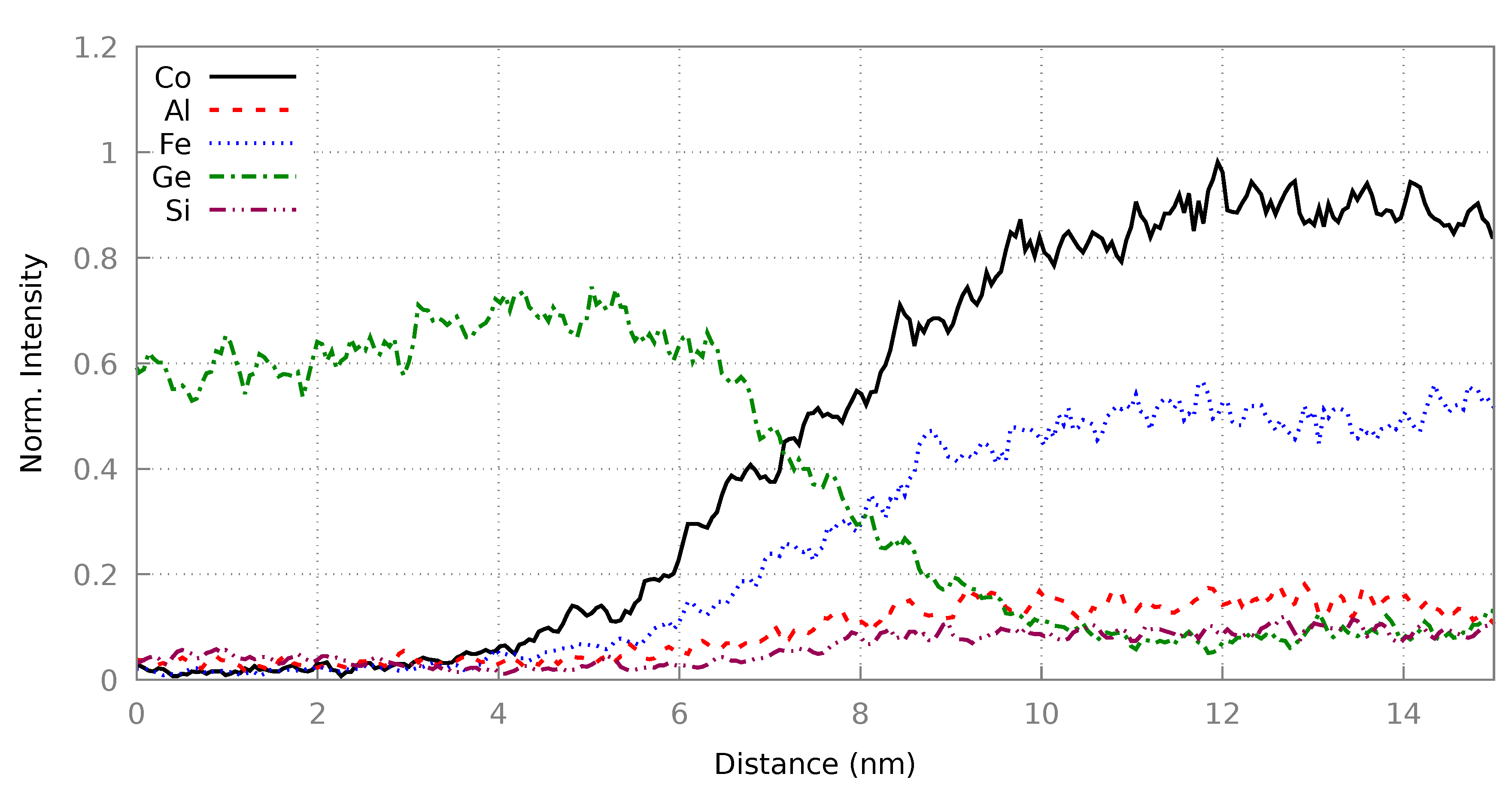
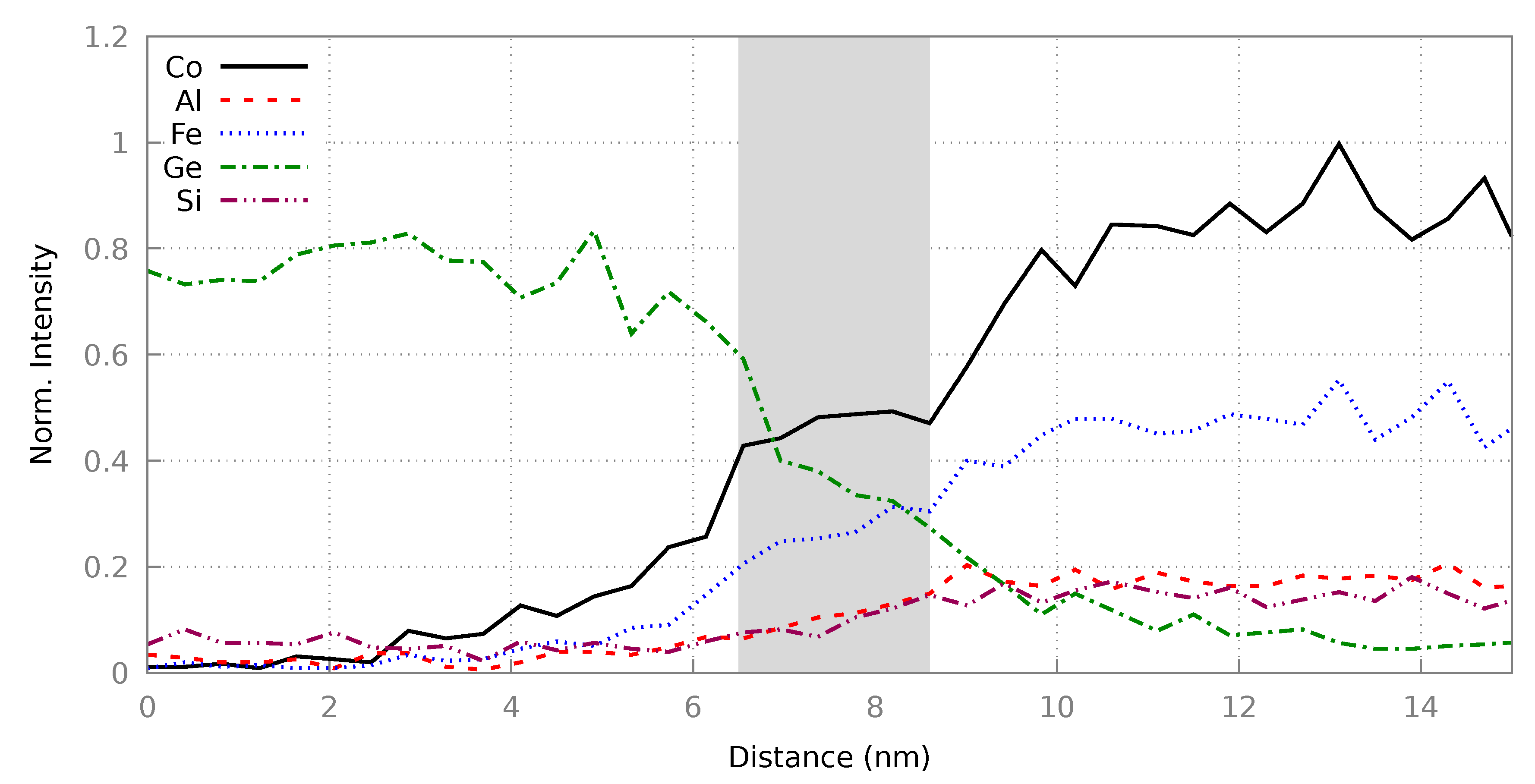
2.4.2. CFAS/n-Ge Interface
3. Results and Discussion
3.1. LJ+S
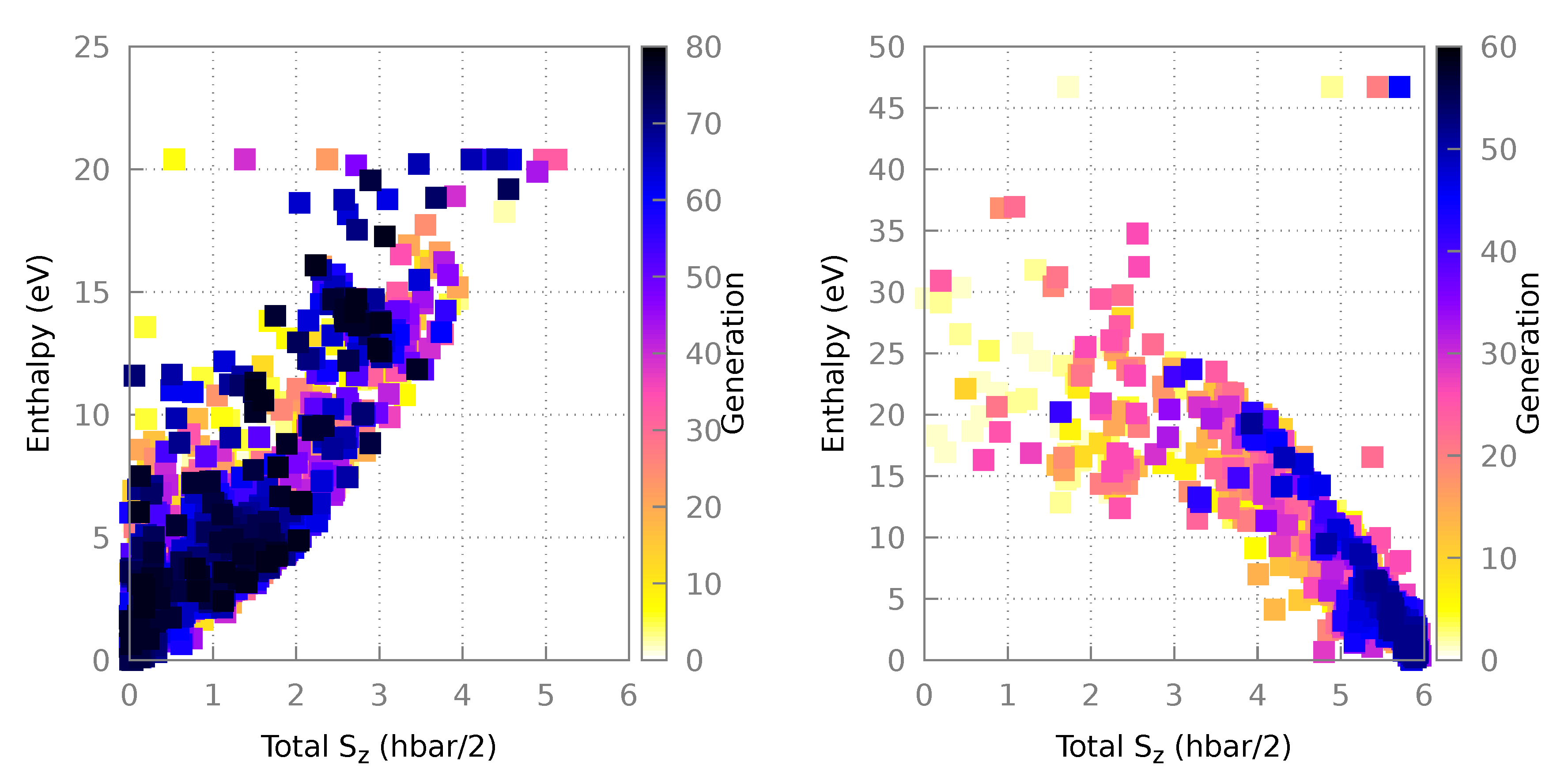
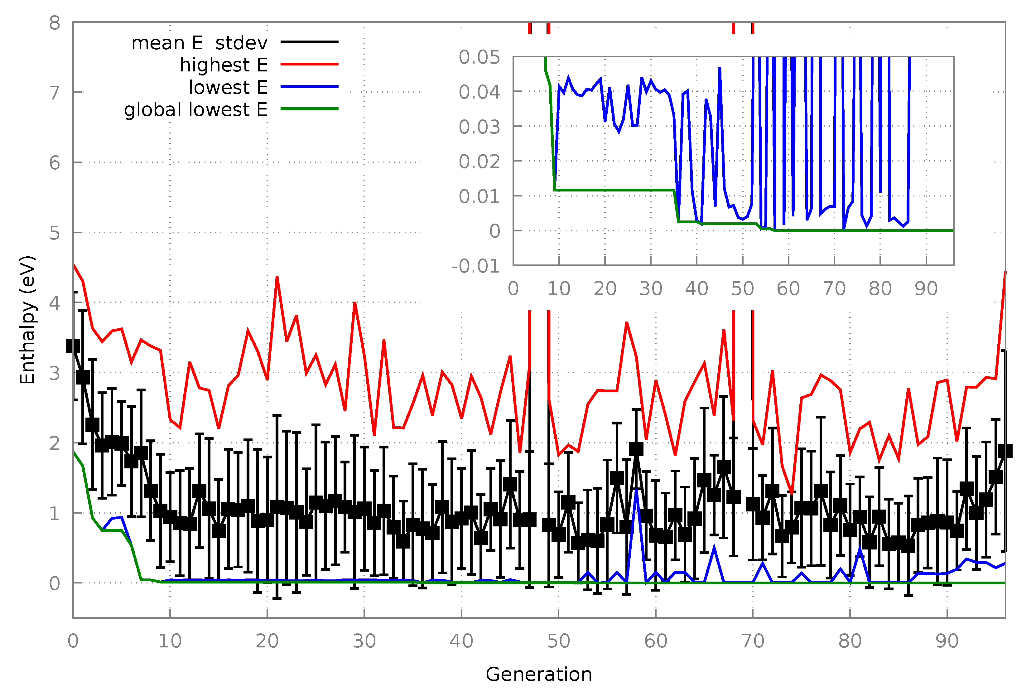
3.1.1. Algorithm Performance
3.1.2. Final Structures
3.2. Heusler/Ge Interface
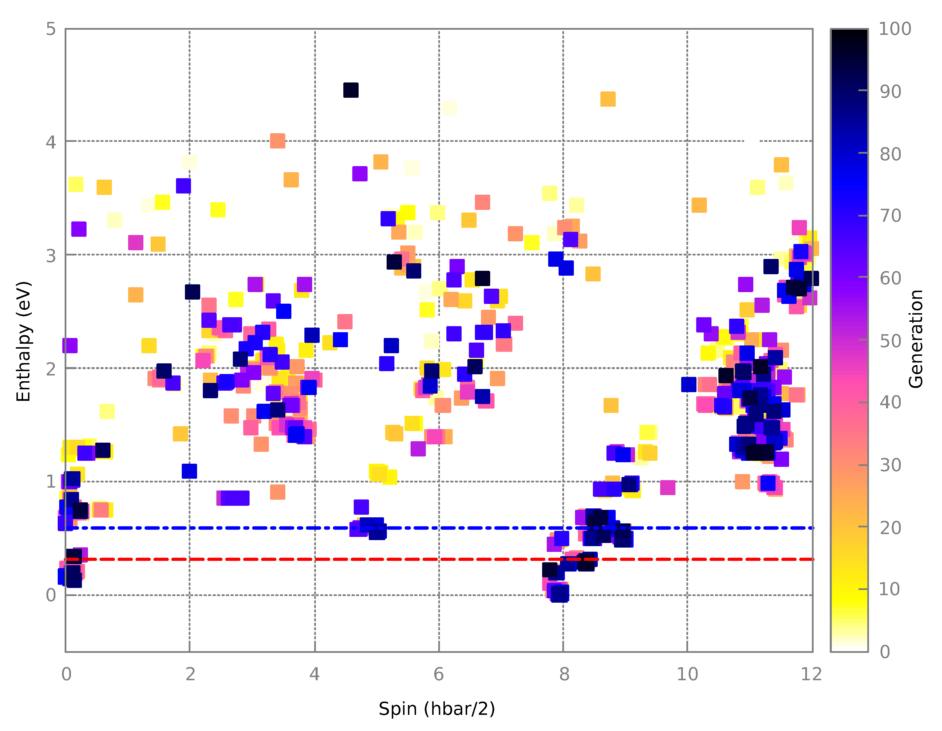
3.2.1. Algorithm Performance
3.2.2. Resultant Structures
4. Conclusions
Author Contributions
Funding
Acknowledgments
Conflicts of Interest
Abbreviations
| CFAS | CoFeAlSi (cobalt iron aluminium silicide; a half-metallic Heusler alloy) |
| DFT | Density Functional Theory |
| GA | Genetic Algorithm |
| LJ | Lennard-Jones |
| LJ+S | Lennard-Jones with spin |
| EDS | Energy dispersive X-ray spectroscopy |
| DoS | Density of States |
References
- Comstock, R.L. Review modern magnetic materials in data storage. J. Mater. Sci. Mater. Electron. 2002, 13, 509–523. [Google Scholar] [CrossRef]
- Weller, D.; Parker, G.; Mosendz, O.; Lyberatos, A.; Mitin, D.; Safonova, N.Y.; Albrecht, M. Review article: FePt heat assisted magnetic recording media. J. Vac. Sci. Technol. B 2016, 34, 060801. [Google Scholar] [CrossRef]
- Balke, B.; Wurmehl, S.; Fecher, G.H.; Felser, C.; Kübler, J. Rational design of new materials for spintronics: Co2FeZ ( Z = Al, Ga, Si, Ge). Sci. Technol. Adv. Mater. 2008, 9, 014102. [Google Scholar] [CrossRef] [PubMed]
- Li, X.; Yang, J. First-principles design of spintronics materials. Natl. Sci. Rev. 2016, 3, 365–381. [Google Scholar] [CrossRef]
- Coey, J. Rare-earth magnets. Endeavour 1995, 19, 146–151. [Google Scholar] [CrossRef]
- Alonso, E.; Sherman, A.M.; Wallington, T.J.; Everson, M.P.; Field, F.R.; Roth, R.; Kirchain, R.E. Evaluating rare earth element availability: A case with revolutionary demand from clean technologies. Environ. Sci. Technol. 2012, 46, 3406–3414. [Google Scholar] [CrossRef] [PubMed]
- Wales, D.J.; Scheraga, H.A. Global optimization of clusters, crystals, and biomolecules. Science 1999, 285, 1368–1372. [Google Scholar] [CrossRef] [PubMed]
- Amsler, M.; Goedecker, S. Crystal structure prediction using the minima hopping method. J. Chem. Phys. 2010, 133, 224104. [Google Scholar] [CrossRef] [Green Version]
- Panosetti, C.; Krautgasser, K.; Palagin, D.; Reuter, K.; Maurer, R.J. Global materials structure search with chemically motivated coordinates. Nano Lett. 2015, 15, 8044–8048. [Google Scholar] [CrossRef]
- Pickard, C.J.; Needs, R.J. Ab initio random structure searching. J. Phys. Condens. Matter 2011, 23, 053201. [Google Scholar] [CrossRef]
- Woodley, S.M.; Catlow, R. Crystal structure prediction from first principles. Nat. Mater. 2008, 7, 937–946. [Google Scholar] [CrossRef] [PubMed]
- Wang, Y.; Lv, J.; Zhu, L.; Ma, Y. Crystal structure prediction via particle-swarm optimization. Phys. Rev. B 2010, 82, 094116. [Google Scholar] [CrossRef] [Green Version]
- Woodley, S.M.; Battle, P.D.; Gale, J.D.; Richard, A.; Catlow, C. The prediction of inorganic crystal structures using a genetic algorithm and energy minimisation. Phys. Chem. Chem. Phys. 1999, 1, 2535–2542. [Google Scholar] [CrossRef]
- Abraham, N.L.; Probert, M.I.J. A periodic genetic algorithm with real-space representation for crystal structure and polymorph prediction. Phys. Rev. B 2006, 73, 224104. [Google Scholar] [CrossRef] [Green Version]
- Glass, C.W.; Oganov, A.R.; Hansen, N. USPEX—Evolutionary crystal structure prediction. Comput. Phys. Commun. 2006, 175, 713–720. [Google Scholar] [CrossRef]
- Lonie, D.C.; Zurek, E. XtalOpt: An open-source evolutionary algorithm for crystal structure prediction. Comput. Phys. Commun. 2011, 182, 372–387. [Google Scholar] [CrossRef]
- Lennard-Jones, J.E. Cohesion. Proc. Phys. Soc. 1931, 43, 461. [Google Scholar] [CrossRef]
- Hohenberg, P.; Kohn, W. Inhomogeneous electron gas. Phys. Rev. 1964, 136, B864–B871. [Google Scholar] [CrossRef]
- Kohn, W.; Sham, L.J. Self-Consistent equations including exchange and correlation effects. Phys. Rev. 1965, 140, A1133–A1138. [Google Scholar] [CrossRef]
- Payne, M.C.; Teter, M.P.; Allan, D.C.; Arias, T.A.; Joannopoulos, J.D. Iterative minimization techniques for ab initio total-energy calculations: Molecular dynamics and conjugate gradients. Rev. Mod. Phys. 1992, 64, 1045–1097. [Google Scholar] [CrossRef]
- Woods, N.; Payne, M.; Hasnip, P. Computing the self-consistent field in Kohn-Sham density functional theory. J. Phys. Condens. Matter 2019, 31, 453001. [Google Scholar] [CrossRef] [PubMed]
- Perdew, J.P.; Burke, K.; Ernzerhof, M. Generalized gradient approximation made simple. Phys. Rev. Lett. 1996, 77, 3865–3868. [Google Scholar] [CrossRef] [PubMed]
- Jones, R.O.; Gunnarsson, O. The density functional formalism, its applications and prospects. Rev. Mod. Phys. 1989, 61, 689–746. [Google Scholar] [CrossRef]
- Hasnip, P.J.; Refson, K.; Probert, M.I.J.; Yates, J.R.; Clark, S.J.; Pickard, C.J. Density functional theory in the solid state. Philos. Trans. R. Soc. A Math. Phys. Eng. Sci. 2014, 372. [Google Scholar] [CrossRef] [PubMed]
- Abraham, N.; Probert, M. Improved real-space genetic algorithm for crystal structure and polymorph prediction. Phys. Rev. B 2008, 77, 134117. [Google Scholar] [CrossRef] [Green Version]
- Abraham, N.L.; Probert, M.I.J. Erratum: Improved real-space genetic algorithm for crystal structure and polymorph prediction [Phys. Rev. B 77, 134117 (2008)]. Phys. Rev. B 2016, 94, 059904. [Google Scholar] [CrossRef]
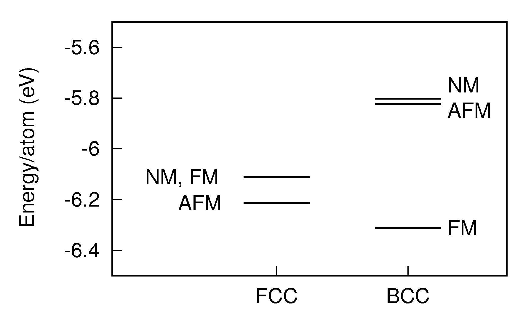
- Kübler, J. Magnetic moments of ferromagnetic and antiferromagnetic bcc and fcc iron. Phys. Lett. A 1981, 81, 81–83. [Google Scholar] [CrossRef]
- Hirshfeld, F.L. Bonded-atom fragments for describing molecular charge densities. Theor. Chim. Acta 1977, 44, 129–138. [Google Scholar] [CrossRef]
- Clark, S.J.; Segall, M.D.; Pickard, C.J.; Hasnip, P.J.; Probert, M.I.; Refson, K.; Payne, M.C. First principles methods using CASTEP. Z. Für Krist.-Cryst. Mater. 2005, 220, 567–570. [Google Scholar] [CrossRef] [Green Version]
- Bacon, G. Neutron Diffraction Monographs on the Physics and Chemistry of Materials; Oxford University Press: New York, NY, USA, 1975. [Google Scholar]
- Harrison, R.J.; Krasko, G.L. Magnetic-state-dependent interatomic potential for iron (abstract). J. Appl. Phys. 1990, 67, 4585. [Google Scholar] [CrossRef]
- Dudarev, S.L.; Derlet, P.M. A ‘magnetic’ interatomic potential for molecular dynamics simulations. J. Phys. Condens. Matter 2005, 17, 7097. [Google Scholar] [CrossRef]
- Ackland, G.J. Two-band second moment model for transition metals and alloys. J. Nucl. Mater. 2006, 351, 20–27. [Google Scholar] [CrossRef] [Green Version]
- Dragoni, D.; Daff, T.D.; Csányi, G.; Marzari, N. Achieving DFT accuracy with a machine-learning interatomic potential: Thermomechanics and defects in bcc ferromagnetic iron. Phys. Rev. Mater. 2018, 2, 013808. [Google Scholar] [CrossRef] [Green Version]
- Nedelkoski, Z.; Hasnip, P.J.; Sanchez, A.M.; Kuerbanjiang, B.; Higgins, E.; Oogane, M.; Hirohata, A.; Bell, G.R.; Lazarov, V.K. The effect of atomic structure on interface spin-polarization of half-metallic spin valves: Co2MnSi/Ag epitaxial interfaces. Appl. Phys. Lett. 2015, 107, 212404. [Google Scholar] [CrossRef]
- Kuerbanjiang, B.; Fujita, Y.; Yamada, M.; Yamada, S.; Sanchez, A.M.; Hasnip, P.J.; Ghasemi, A.; Kepaptsoglou, D.; Bell, G.; Sawano, K.; et al. Correlation between spin transport signal and Heusler/semiconductor interface quality in lateral spin-valve devices. Phys. Rev. B 2018, 98, 115304. [Google Scholar] [CrossRef] [Green Version]
- Stukowski, A. Visualization and analysis of atomistic simulation data with OVITO—The open visualization tool. Model. Simul. Mater. Sci. Eng. 2009, 18, 015012. [Google Scholar] [CrossRef]


| Parameter | Value |
|---|---|
| 1.75 eV | |
| 1.87 Å | |
| A | −2.82 eV |
| 0.83 Å |
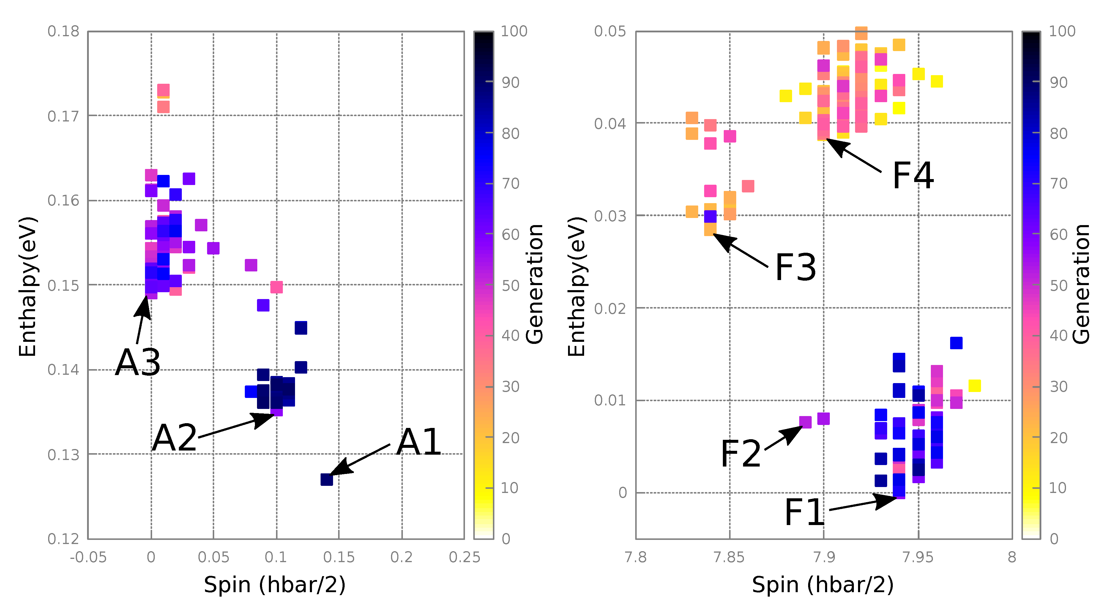
| Structure | Enthalpy (eV) | Total Spin () | Total |Spin|() | Disorder |
|---|---|---|---|---|
| F1 | 0.0 | 7.94 | 9.91 | None |
| F2 | 0.01 | 7.89 | 9.89 | None |
| F3 | 0.03 | 7.84 | 9.92 | Ge ↔ Si |
| F4 | 0.04 | 7.89 | 9.93 | Ge ↔ Si |
| A1 | 0.13 | 0.13 | 7.50 | 2Ge ↔ Si,Fe |
| A2 | 0.14 | 0.10 | 7.45 | Ge ↔ Fe |
| A3 | 0.15 | 0.00 | 7.62 | None |
© 2019 by the authors. Licensee MDPI, Basel, Switzerland. This article is an open access article distributed under the terms and conditions of the Creative Commons Attribution (CC BY) license (http://creativecommons.org/licenses/by/4.0/).
Share and Cite
Higgins, E.J.; Hasnip, P.J.; Probert, M.I.J. Simultaneous Prediction of the Magnetic and Crystal Structure of Materials Using a Genetic Algorithm. Crystals 2019, 9, 439. https://doi.org/10.3390/cryst9090439
Higgins EJ, Hasnip PJ, Probert MIJ. Simultaneous Prediction of the Magnetic and Crystal Structure of Materials Using a Genetic Algorithm. Crystals. 2019; 9(9):439. https://doi.org/10.3390/cryst9090439
Chicago/Turabian StyleHiggins, Edward J., Phil J. Hasnip, and Matt I.J. Probert. 2019. "Simultaneous Prediction of the Magnetic and Crystal Structure of Materials Using a Genetic Algorithm" Crystals 9, no. 9: 439. https://doi.org/10.3390/cryst9090439
APA StyleHiggins, E. J., Hasnip, P. J., & Probert, M. I. J. (2019). Simultaneous Prediction of the Magnetic and Crystal Structure of Materials Using a Genetic Algorithm. Crystals, 9(9), 439. https://doi.org/10.3390/cryst9090439