Application of Fundamental Models for Creep Rupture Prediction of Sanicro 25 (23Cr25NiWCoCu)

Abstract

Creep rupture prediction is always a critical matter for materials serving at high temperatures and stresses for a long time. Empirical models are frequently used to describe creep rupture, but the parameters of the empirical models do not have any physical meanings, and the model cannot reveal the controlling mechanisms during creep rupture. Fundamental models have been proposed where no fitting parameters are involved. Both for ductile and brittle creep rupture, fundamental creep models have been used for the austenitic stainless steel Sanicro 25 (23Cr25NiWCoCu). For ductile creep rupture, the dislocation contribution, solid solution hardening, precipitation hardening, and splitting of dislocations were considered. For brittle creep rupture, creep cavitation models were used taking grain boundary sliding, formation, and growth of creep cavities into account. All parameters in the models have been well defined and no fitting is involved. MatCalc was used for the calculation of the evolution of precipitates. Some physical parameters were obtained with first-principles methods. By combining the ductile and brittle creep rupture models, the final creep rupture prediction was made for Sanicro 25. The modeling results can predict the experiments at long-term creep exposure times in a reasonable way.

1. Introduction

The concept of Advanced Ultra-supercritical (AUSC) power plants has been proposed world-wide in order to raise the operating temperature and stress for fossil-fired power plants [1]. Thereby, the efficiency of the power plants can be improved and the CO₂ emissions can be reduced. In the AUSC conditions, the temperature is 700 °C or more and the stress is above 30 MPa, which imposes high requirements on the materials used for power plants. Austenitic stainless steels and nickel-based superalloys are candidate materials for the critical components serving at high temperature and stress. Sanicro 25 (23Cr25NiWCoCu, also called UNS S31035) is an austenitic stainless steel developed by Sandvik [2,3,4,5] and is designed for use in steam boilers at high temperatures. The design life of power plants nowadays is 20 to 30 years, and their actual life can be even longer. The high temperatures and stresses give rise to a slow mechanical deformation that is called creep, which will eventually result in rupture. This type of deformation is life controlling for many components in fossil-fired power plants. Since the creep deformation is time dependent, it is crucial to understand its long-term behavior and the mechanisms involved.

Experimental tests are the most accurate means to characterize and assess the creep rupture life of materials. To generate proper design data, tests must run over many years. Still, the results have to be extrapolated by a large factor in time to reach the desired design life. Therefore, predicting the long-term creep rupture life of materials has been a critical issue. Traditionally, the creep rupture life has been extrapolated with empirical models. A wide range of Time-Temperature-Parameters have been proposed for this purpose, like the Larson-Miller parameter [6]. ECCC has proposed a Master Equation for different types of materials, where several parameters are involved [7,8]. Empirical models for creep strain versus time curves have also been developed such as the θ and Ω models, where the model can represent the creep curves in a good way [9]. However, the nature of these models is to fit the current existing experimental results and with the parameters obtained to extrapolate the future creep rupture life. The more parameters, the more accurately the models can fit with the experiments. However, the parameters involved in these empirical models do not have any physical meanings in most cases. The models are just a means of fitting data. They do not provide any basic understanding for the creep behavior and cannot reveal the rupture controlling mechanisms. In the work within ECCC, it has been found that the empirical models only can be used to extrapolate by up to a factor of three in time with reasonable precision. The reason is most likely that the empirical models cannot represent the operating failure mechanisms in a reliable way.

For materials serving at high temperatures and stresses, long-term life safety is a crucial factor. One needs to understand the mechanism for better prediction of the creep rupture life. To resolve the problems with the empirical models, Sandström has proposed the use of fundamental models [9,10]. Since fundamental models mean different things to different scientists, a definition of what is meant in the present context has been provided.

(a)

The models should be able to represent the rupture controlling mechanism;

(b)

All parameters in the models should be well-defined;

(c)

No fitting or adjustable parameters should be used to describe the experimental mechanical data;

(d)

The modelling results should be sufficiently precise in order to be used technically.

The nature of the fundamental creep models is to predict the macro creep rupture strength by considering the evolution of microstructure and defects during the creep process. Fundamental models have been used successfully for creep rupture prediction of Cu and austenitic stainless steels [10,11,12,13]. The models that are taken into account are summarized below.

This paper aims to use fundamental models for predicting the creep rupture strength of Sanicro 25. The ductile creep rupture models, including dislocation contribution, precipitation hardening, solid solution hardening, and splitting of dislocation will be used. On the other hand, the brittle creep rupture due to formation, growth, and coalescence of grain boundary cavities will also be considered. By combining the ductile and brittle creep rupture models, the final creep rupture strength prediction will be made, and the modeling results will be compared to experimental data for Sanicro 25.

There are some new features in the modelling of the rupture. Recently, our model for precipitation hardening (PH) has been updated and further developed [14]. The new model can describe a number of features of the influence of Co particles on the creep strength of copper. Since the PH is the main contribution to the creep strength in this case, this is a direct verification of the PH model. This model has been implemented in the present paper. To compute the rupture elongation for ductile rupture has always been a challenge. However, it has been accomplished recently for copper taking recovery and necking during tertiary creep into account [15]. Results from this analysis have been used in the present work.

2. Models and Materials

Creep rupture can either take place due to ductility exhaustion or due to embrittlement. The former mechanism is referred to as ductile creep rupture and is controlled by the formation, movement, and recovery of dislocations. The second mechanism is called brittle rupture. While many mechanisms can give rise to embrittlement of materials but in commercial materials for high-temperature service, brittle rupture is primarily controlled by cavity formation and development. Ductile rupture is analyzed in Section 2.1 and brittle rupture in Section 2.2.

2.1. Ductile Creep Rupture Models

Fundamental creep models for ductile rupture based on dislocation mechanisms have been formulated and shown to be able to describe the rupture behavior accurately, for example, for austenitic stainless steels [10,11,12,16]. Since the creep strength is influenced by precipitation hardening and solid solution hardening, it is important to take their role into account. Besides, due to the low stacking fault energy (SFE) in austenitic stainless steels, the effect of partial dislocations is considered. The final form of the ductile creep rupture models can be expressed as:

$${\dot{\epsilon }}_{cr}=\frac{2bK{\tau }_L}{\alpha m^2}{M}_{clgl}\left(T,\sigma \right){\left(\frac{\sigma -{\sigma }_{PH}}{\alpha mGb}\right)}^3{f}_{SFE},$$

(1)

where ${\dot{\epsilon }}_{cr}$ is the creep rate, b is Burgers’ vector, and K is the constant related to subgrain size, which is shown in Section 2.2 Brittle creep rupture models, Equation (15). α is a work-hardening constant, and m is the Taylor factor, which is about 3.06 for fcc materials. M_clgl (T, σ) is the glide and climb mobility of dislocations, and f_SFE is the stacking fault energy factor. σ is the applied stress, T is the absolute temperature, and G the shear modulus. σ_PH is the precipitation hardening strength. Rupture is assumed to take place when a certain creep strain (rupture elongation) has been reached.

M_clgl (T, σ), σ_PH and f_SFE will be introduced separately now.

2.1.1. Stacking Fault Energy Factor f_SFE

The presence of partial dislocations reduces the creep rate since split dislocations climb at a lower rate. This effect increases with the width of the split dislocations, which is inversely proportional to the stacking fault energy. The creep rate is reduced by a factor f_SFE [17]:

$$f_{SFE}=2{\left(\frac{24\pi \left(1-\nu \right)}{2+\nu }\right)}^2{\left(\frac{{\gamma }_{SFE}}{Gb}\right)}^2,$$

(2)

where ν is the Poisson’s ratio, γ_SFE is the stacking fault energy, G the shear modulus, and b Burgers’ vector. Vitos et al. [18,19] have studied the stacking fault energy of austenitic stainless steels with quantum mechanical first-principles methods. Using their results, the stacking fault energy for 23Cr25NiWCuCo is found to be about 0.044 J/m².

2.1.2. Precipitation Hardening

Precipitation hardening is often the most potent way of increasing the creep strength. For a long time, no good way of computing the magnitude of this strength contribution was available. In general, the room temperature value of the Orowan strength was used. However, this expression usually strongly overestimates the precipitation hardening. In addition, it could not reproduce the observed exponential decrease with increasing temperature. For this reason, a new expression for the precipitation hardening strength σ_PH was developed [9,10,16,20,21]:

$${\sigma }_{PH}=0.8\frac{G{b}^{2}m}{b{\lambda }_{rc}},$$

(3)

G is the shear modulus, b the Burgers’ vector, and m the Taylor factor. λ_rc is the particle spacing corresponds to particles exceeding a critical radius r_c. When the particle radius is smaller than r_c, there will be sufficient time for dislocations to climb across them and they will not contribute to the creep strength. The critical particle radius r_c can be expressed as:

$$2r_c=t_{climb}{v}_{disl},$$

(4)

which is the climb time of the dislocations across the particles multiplied with the dislocation climb velocity v_disl. t_climb is assumed to be a significant fraction of the design life. The climb velocity of dislocations can be obtained from:

$$v_{disl}=b{M}_{climb}\sigma ,$$

(5)

where σ is the applied stress. M_climb is the climb mobility of dislocations, which can be expressed as:

$$M_{climb}\left(T,\sigma \right)=\frac{D_{s0}b}{k_{B}T}exp\left(\frac{(\sigma -{\sigma }_{PH})b^3}{k_{B}T}\right)exp\left\{-\frac{Q_{self}}{R_{g}T}\right\}/f_{sol},$$

(6)

where D_so is the pre-exponential coefficient for self-diffusion, k_B is the Boltzmann’s constant, T is the absolute temperature, R_g is the gas constant, and Q_self is the activation energy for self-diffusion. f_sol is a factor that takes solid solution hardening of alloying elements into account. f_sol will be introduced later in this section.

The particle spacing λ_rc can be related to the number of precipitates N_part per unit area exceeding the critical size r_c:

$${\lambda }_{rc}=\frac{1}{\sqrt{N_{part}}}.$$

(7)

The thermodynamic software MatCalc [16,22] was used to calculate the dimensions of the precipitates. The number of precipitates N_part with radii larger than r_c can be computed if the often observed exponential particle distribution is assumed [16,20,21,22]:

$$N_{part}=N_{part}^0{\mathrm{e}}^{-k_r{r}_c},$$

(8)

where $k_r=1/\overline{r}$, and $\overline{r}$ is the average particle radius corresponding to the total number of precipitates contributing to the strengthening $N_{part}^0$, which is a reference state of particles. With the help of MatCalc calculations and Equations (4)–(8), one can get the average particle spacing λ_rc. With Equation (3), one can find the precipitation hardening strength.

2.1.3. Glide and Climb Mobility of Dislocations

The glide and climb mobility of dislocations can be written as:

$$M_{clgl}\left(T,\sigma \right)=\frac{D_{s0}b}{k_{B}T}exp\left(\frac{(\sigma -{\sigma }_{PH})b^3}{k_{B}T}\right)exp\left\{-\frac{Q_{self}}{R_{g}T}\left[1-{\left(\frac{\sigma -{\sigma }_{PH}}{{\sigma }_{imax}}\right)}^2\right]\right\}/f_{sol},$$

(9)

where D_so is the pre-exponential coefficient for self-diffusion, b is the Burgers’ vector, k_B is the Boltzmann’s constant, T is the absolute temperature, σ is the applied stress, σ_PH is the precipitation hardening strength, R_g is the gas constant, and Q_self is the activation energy for self-diffusion. σ_imax is the tensile strength at ambient temperature. f_sol is a factor that takes solid solution hardening of alloying elements into account.

2.1.4. Solid Solution Hardening

The solute atoms interact with dislocations, which will reduce the creep rate. So, a factor f_sol is taken into account for the creep rate [9,11,23]:

$$f_{sol}=\exp \left(\frac{Q_{sol}}{R_{g}T}\right),$$

(10)

where R_g is the gas constant and T the absolute temperature. Q_sol is the activation energy for solid solution hardening. Q_sol is taken as the maximum interaction energy between different alloying elements and dislocations. The interaction energy of different elements with dislocations can be expressed as (in J mol⁻¹) [9,11,23]:

$$U_i^{max}=\frac{\left(1+\nu \right)G{\Omega }_0{\epsilon }_i}{\pi \left(1-\nu \right)},$$

(11)

where ε_i is the linear atomic size misfit, which can be obtained from the first-principles calculations, ν is the Poisson’s ratio, G the shear modulus and Ω₀ the atomic volume. According to first-principles calculations for Sanicro 25, the ε_i of Nb is the maximum one, which is about 25.3% at 1000 K [11]. With the help of Equations (10) and (11), one can get the solid solution hardening factor.

Ductile creep rupture is assumed to happen when the creep strain reaches a critical value ε_crit; then the rupture time can be obtained by:

$$t_{ductrup}=\frac{{\epsilon }_{crit}}{{\dot{\epsilon }}_{cr}}.$$

(12)

With Equations (1)–(12), one can get the ductile creep rupture.

The critical rupture strain can be predicted with basic models. This has been done for annealed and cold worked copper [15,24] describing primary, secondary, and tertiary creep. In particular, the representation of tertiary creep has turned out to be a challenge. Unexpectedly, it has been found that enhanced recovery is the main contribution to tertiary creep. Unfortunately, no detailed analysis seems to have been performed for austenitic stainless steels. Published creep curves for Sanicro 25 [25] show the same tertiary behavior as for cold worked copper, indicating that enhanced recovery is the main mechanism. In addition, the strain during primary creep is quite small. In our model, ε_crit represents the strain in the secondary stage. The total experimental rupture strains are about 40–50% at higher stresses [2,25], and these are clear values for ductile rupture. Considering a significant part from tertiary creep, ε_crit has been taken as 0.2 in the model. This value has also been found to be applicable to other austenitic stainless steels [10].

2.2. Brittle Creep Rupture Models

2.2.1. Grain Boundary Sliding (GBS) Models

In practice, brittle creep rupture takes place as intergranular fracture in commercial austenitic stainless steels. It results from the formation, growth, and coalescence of creep cavities on grain boundaries. Creep cavities are formed by grain boundary sliding (GBS). Two grain boundary sliding models have been proposed for austenitic stainless steels [22]. The final form of the GBS models can be written as:

$$v_{sd}=C_s\dot{\epsilon },$$

(13)

where $v_{sd}$ is the grain boundary sliding displacement rate, C_s is the grain boundary sliding parameter and $\dot{\epsilon }$ is the creep rate. In the shear sliding model, the C_s is related to the grain size. In the shear crack model, the GBS displacement rate is associated with the particle diameter and particle spacing. The particle dimensions in the present paper have been obtained with the help of the thermodynamic software MatCalc.

2.2.2. Cavity Formation Models

He and Sandström have proposed a model for cavity nucleation at substructures [26]. It is assumed that when the particles or subboundary corners on one side of a sliding grain boundary meet the subboundaries on the opposite side of a sliding grain boundary, cavities will be generated. The final form of the nucleation rate dn/dt can be expressed as:

$$\frac{dn}{dt}=\frac{0.9C_s}{d_{sub}}(\frac{1}{{\lambda }^2}+\frac{1}{d_{sub}^2}){\dot{\epsilon }}_{cr}=B{\dot{\epsilon }}_{cr}.$$

(14)

0.9 is a factor due to the average angle between the grain boundary and the sliding direction. λ is the particle spacing, d_sub is the subgrain size, and ${\dot{\epsilon }}_{cr}$ is the creep rate. The final form reproduces experimental observations quite well. The cavity nucleation rate is proportional to the creep rate and can be related to the creep rate with the parameter B. It is well established that the subgrain size is inversely proportional to the applied stress:

$$d_{sub}=\frac{KGb}{\sigma },$$

(15)

where K is about 20 for austenitic stainless steels. Equation (15) is in good agreement with experiments [26].

2.2.3. Creep Cavity Growth Models

For growth of creep cavities, a new model has been proposed based on the constrained creep cavity growth models.

$$\frac{dR}{dt}=2D_0{K}_f\left({\sigma }_{red}-{\sigma }_0\right)\frac{1}{R^2},$$

(16)

where σ_red is the reduced stress:

$${\sigma }_{red}={\sigma }_0+\frac{L^{2}d\beta {\dot{\epsilon }}_{cr}}{32D_0{K}_f}.$$

(17)

In Equations (16) and (17), R is the cavity radius in the grain boundary plane, D₀ is the grain boundary diffusion parameter, D₀ = δD_GBΩ₀/k_BT, where δ is the grain boundary width, D_GB is the grain boundary self-diffusion coefficient, Ω₀ is the atomic volume, k_B is Boltzmann’s constant, and T is the absolute temperature. σ₀ is the sintering stress, σ₀ = 2γ_surf sin(θ)/R, where γ_surf is the free surface energy per unit area and θ is the cavity tip angle. L is the cavity spacing, d is the grain size, ${\dot{\epsilon }}_{cr}$ is the creep rate and β is a material constant (β = 1.8 for homogeneous materials). K_f is a function of the cavitated area fraction f_a [27].

$$K_f=\frac{1}{-2log{f}_a-\left(1-f_a\right)\left(3-f_a\right)},$$

(18)

where f_a = (2R/L)² is the area fraction of the cavitated grain boundaries. The cavity spacing L can be obtained from the number of cavities per unit grain boundary area n_cav:

$$L=1/\sqrt{n_{cav}}.$$

(19)

2.2.4. Brittle Creep Rupture

It is assumed that brittle creep rupture happens when the cavitated area fraction on grain boundaries reaches a critical value A_flim, which can be taken as 25%. The reason for choosing this value has been explained in detail in [27]. The condition for brittle creep rupture to happen can be written as:

$$A_f={{\displaystyle \int }}_{t_i}^t\frac{d{n}_{cav}}{d{t}_1}\left(t_1\right)\pi R^2\left(t,t_1\right)d{t}_1<A_{flim},$$

(20)

where R(t,t₁) is the cavity radius at time t that was formed at time t₁, n_cav is the cavity number density, which can be obtained from Equation (14). t_i is an incubation time that is about one-third of the rupture time, as shown in [28] for example. Thus, with a combination of the creep cavity nucleation models and the modified cavity growth models, the brittle rupture due to creep cavitation could be predicted.

By combining the ductile and brittle creep rupture models, the final creep rupture can be obtained. Now the models described above, Equations (1)–(20) will be used for creep rupture prediction of Sanicro 25.

2.3. Experimental Data Sources

Experimental creep rupture data for Sanicro 25 was extracted from [2,5,25]. Experimental data for dimensions of precipitates was from [2,5,25] where particle radius and number density had been characterized. During the MatCalc calculation and the modeling process, the grain size was taken as 25 µm, which is consistent with metallography observations [25]. In the MatCalc simulation, the chemical composition was set according to

Table 1. Chemical composition of Sanicro 25 (23Cr25NiWCoCu) (wt%).

C	Si	Mn	Cr	Ni	N	W	Co	Cu	P	S	Nb	Fe
0.064	0.2	0.5	22.5	25	0.23	3.6	1.5	3.0	0.025	0.015	0.5	Balance

.

3. Results

3.1. Constants Used in the Calculation

The constants and physical parameters used in the calculation for Sanicro 25 are shown below in

Table 2. Constants for Sanicro 25 (23Cr25NiWCuCo) used in the computations.

Parameter Description	Parameter	Value	References
Grain boundary diffusion constant	δDGB	${10}^{-9.87}{e}^{\frac{-218700}{R_{gas}T}}$	[29]
Shear modulus	G	(78 − 0.036 × (T − 273)) × 103 MPa	[30]
Activation energy for self-diffusion	Q	293 kJ mol−1	[31]
Atomic volume	Ω0	1.14 × 10−29 m3	[23]
Boltzmann constant	kB	1.381 × 10−23 J K−1
Burgers’ vector	b	2.58 × 10−10 m
Poisson’s ratio	ν	0.3	[32]
Surface energy	γsurf	2.8 J m−2	[33]
Cavity tip angle	θ	70°	[34]
Pre-exponential coefficient for self-diffusion	Ds0	3.15 × 10−4 m2 s−1	[31]
Taylor factor	m	3.06
Work hardening constant	α	(1 − ν/2)/2π(1 − ν) = 0.19	[35]

.

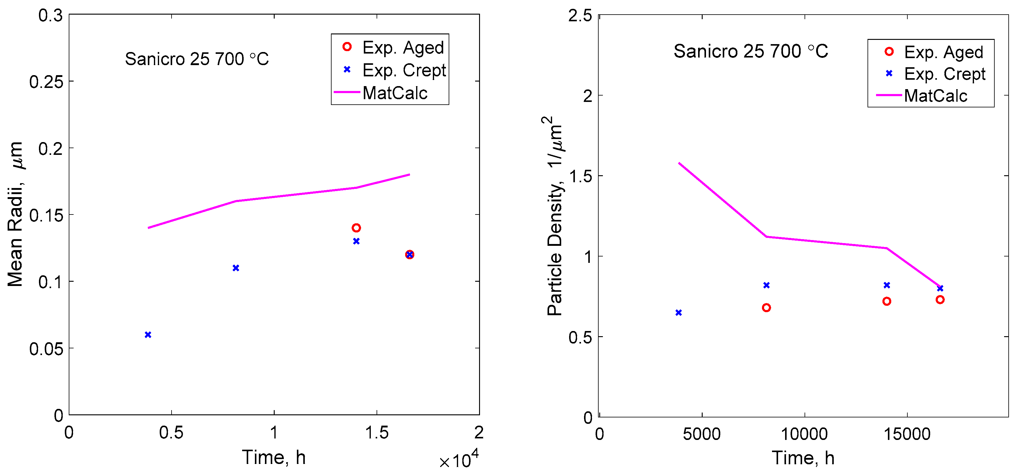
3.2. Precipitation Calculation

For the precipitation hardening, MatCalc was used to calculate the particle dimensions. The setup of MatCalc calculations can be found in [16,22]. For Sanicro 25, the chemical composition during calculation was set according to Table 1. Two sets of particles were considered, which includes Laves phase and M₂₃C₆ precipitates. For the precipitation hardening contribution, the particle radius and number density are needed according to Equations (4)–(8). For the Laves phase, a particle radius of 0.05 µm and a volume fraction of 0.01 were found in reasonable agreement with [2]. For the M₂₃C₆ precipitates nucleation sites were chosen at the grain boundaries. The modeling results of the particle radius and number density were compared to the experimental observations as shown in Figure 1. One can see that the modeling results are within a factor of 2 within the experimental data.

It should be pointed out that the error range of the experimental data for the particle radius and number density usually fluctuate in one order of magnitude as shown in [16,36] for HR3C (25Cr20NiNbN). So, the current results are in acceptable agreement. Besides, the experimental data is limited by the resolution of the equipment and characterization methods.

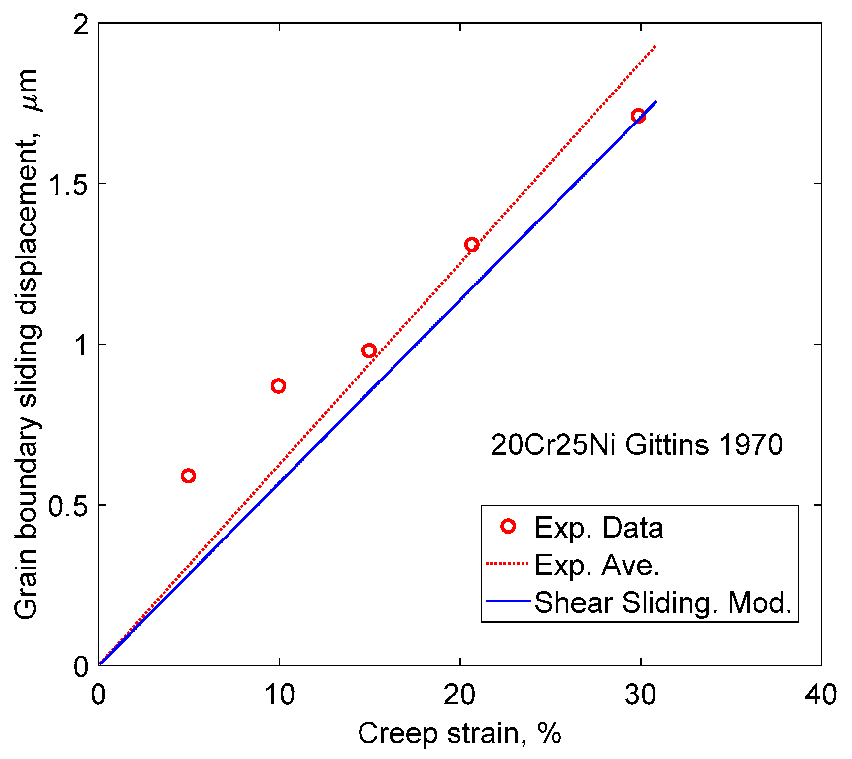
3.3. Grain Boundary Sliding (GBS) Displacement

With the help of the shear sliding model, one can get the GBS parameter C_s. Figure 2 shows the comparison of the shear sliding model and experimental GBS displacement for 20Cr25Ni austenitic stainless steels, which is close to the studied case. A good agreement can be reached for the models and experiments.

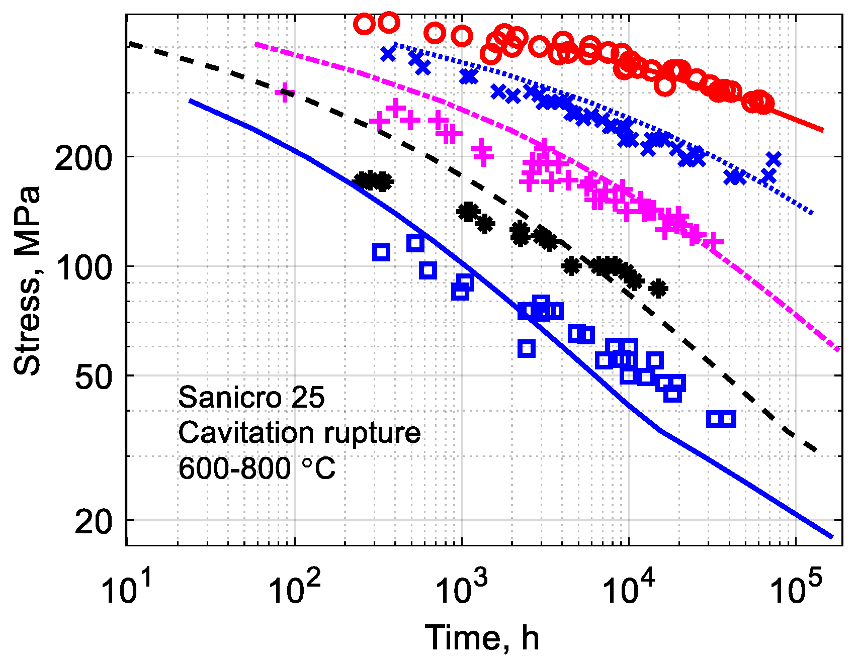
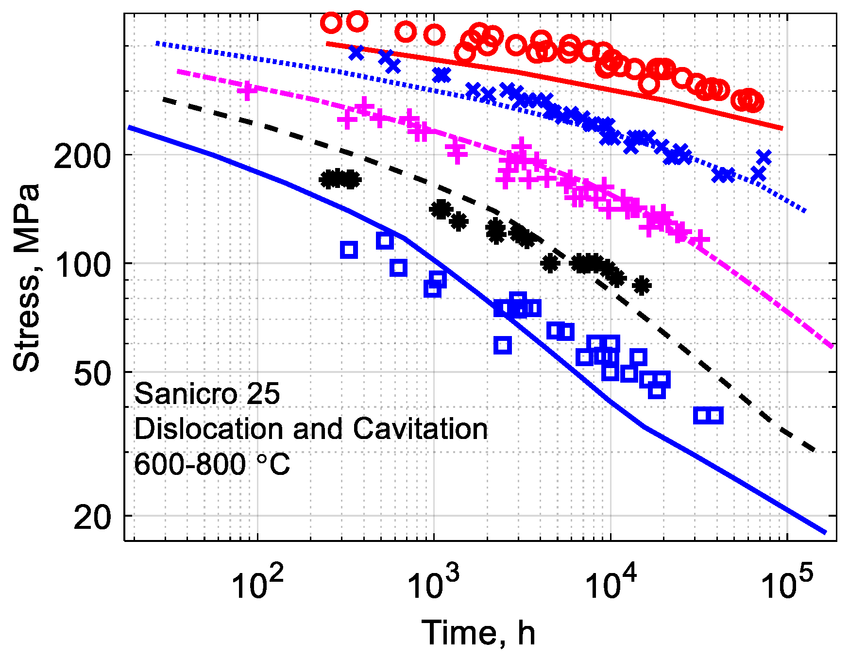
3.4. Creep Rupture Prediction

To predict the creep rupture strength of Sanicro 25, the ductile creep rupture models and brittle creep rupture models are used separately. Then, the results of the two models are compared for prediction. By combining the ductile and brittle creep rupture models, the principle is that the model that gives the shorter time to creep failure is taken as the final creep rupture time. Fully ductile creep rupture occurs by ductile collapse. A plastic instability takes place followed by necking. Necking occurs very close to the rupture [15]. This process can be interrupted by embrittlement in the metal. For commercial austenitic stainless steels, the creep embrittlement is assumed to be induced by cavitation. If the cavitation is fully developed and initiates failure before the plastic collapse, brittle rupture is said to happen. Thus, the failure process that occurs first controls the rupture.

In Figure 3, the ductile creep rupture modeling results are compared to the experimental data. In the model, the contributions from dislocation hardening, precipitation hardening, solid solution hardening, and splitting of dislocations are considered. The modelling results at 600 °C underestimated the creep rupture life. In the temperature ranges of 650–800 °C, the model can predict the rupture times within a factor of 3 at higher stresses within a factor of 1.2 at lower stresses.

Figure 4 shows the creep rupture prediction for the brittle creep rupture model. The prediction results were in the same range with the experiments at 600 °C. At 650–700 °C, the model can predict the rupture times within a factor of 3 at stresses higher than 200 MPa, and in the same range with the experiments at lower stresses. At 750–800 °C, the modelling results were within a factor of 3 with the experiments. At longer creep exposure time, the brittle creep rupture models can give a more conservative prediction. Both models can represent the creep rupture strength of Sanicro 25 in a reasonable way. The creep cavitation model shows a more conservative prediction at long-term creep life, which is often a problematic point now for most empirical models.

By combining the ductile and brittle creep rupture models, one gets the final results for the creep rupture prediction of Sanicro 25, as shown in Figure 5. The combination principle is to take the shorter predicted creep rupture time as the final creep rupture life. Comparing Figure 3 to Figure 5, one can see that there is a transition region in Figure 5, where the ductile and brittle creep rupture region was distinguished. At higher stresses and lower temperatures, the ductile creep rupture prediction based on dislocation mechanism was taken as the final creep rupture life. At lower stresses and higher temperatures, the brittle creep rupture prediction based on creep cavitation was taken as the final modelling results. Thus, one can see that the ductile creep rupture dominates at higher stresses. However, at lower stresses and higher temperatures, the creep is governed by the brittle creep rupture. The final modeling results can represent the creep rupture in a reasonable way.

4. Discussion

The fundamental models shown here are based on the microstructure and defect evolution, where all involved parameters have been well defined and no parameters are fitted to the creep rate. This procedure gives a good understanding of the controlling mechanisms, which improves the accuracy of the results. In the calculation, the main input parameters are applied stress σ and the absolute temperature T.

Some of the parameters have a critical influence on the results. First-principles methods were used to calculate the stacking fault energy of Sanicro 25. Q_sol is the activation energy for solid solution hardening. It is taken as the maximum interaction energy between the dislocations and different alloying elements. The interaction energy is related to the lattice misfit parameters, which can be obtained from first-principles calculations. For Sanicro 25, Nb has the highest interaction energy with dislocations, so its value is taken as the Q_sol. This is different from the empirical models, where the Q_sol value is obtained by fitting the creep rupture data. For ductile creep rupture, the critical strain is taken as 0.2, which is a general value for many austenitic stainless steels. For the grain boundary sliding model, the input parameter is the grain size. The other parameters in the model have specific meanings. For the formation of creep cavities, the parameters involved are subgrain size and particle spacing. The subgrain size can be obtained with Equation (15), where the constants K has been explained in detail in [26]. The temperature dependence of the shear modulus G can be described by the equation in Table 2 [26]. For brittle creep rupture, the critical value for the cavitated area fraction is taken as 0.25. The reason for choosing this value has been explained in [10].

To investigate whether the predicted rupture times are sensitive to the chosen parameter values, some parameters have been varied. The experimental rupture ductility lies in the interval 0.15 to 0.5, covering both ductile and brittle rupture. The rupture elongation 0.2 used in the model refers to the strain in the secondary stage during fully ductile rupture. Taking into account the strain during tertiary creep, the full range of possible values should be between 0.15 and 0.25. Increasing the rupture strain from 0.2 to 0.25 gives an increase in the rupture life for ductile rupture by a factor of 1.25 as expected and a change from 0.2 to 0.15 gives a corresponding decrease. Such a large change can be seen as a small change on the rupture curve but does not modify the general appearance of the results. The cavitated grain boundary area fraction is in close agreement between different sources with a value of 0.25 (see above). If this value is changed by 10%, there is a corresponding change in the rupture times by a factor of 1.1 which is barely visible in the diagrams.

The value for K that controls the subgrain size is quite well established, the same applies to the solution hardening constant Q_sol. The results are quite insensitive to these parameters. A change by 10% in any of these parameters is hardly observable on the rupture curves. A parameter that is more uncertain is the minimum particle size that controls the interparticle spacing, since the metallographic data is limited. A value of 0.05 µm has been assumed in the model. If this value is doubled, the effect on the rupture curve is negligibly small. It can be concluded that the model results are not very sensitive to the chosen parameter values.

The precipitation behavior can be obtained from MatCalc calculations as shown in Figure 1. It should be pointed out that the error range of the experimental data for the particle radius and number density usually fluctuate in one order of magnitude, as shown in [16,36] for HR3C (25Cr20NiNbN), the ratio of the highest/lowest particle radius ranges from 5 to 50. Besides, the accuracy of the experimental data is limited by the resolution of the equipment and characterization methods. As shown in Figure 1, the calculated results are about 1–2 times of the experimental particle dimensions. This shows that the MatCalc calculation results are in acceptable agreement with the experimental observations.

Both intragranular (dimples) and intergranular (cavities) fracture were observed from experimental observations for Sanicro 25 [5,25] representing ductile and brittle rupture. Unfortunately, the details in the literature are few and a detailed comparison to the model is not possible, but the basic mechanisms are the same. Any details about cavity spacing in Sanicro 25 are not available. The model is based on data for other austenitic stainless steels such as TP316. The model can describe these data in a satisfactory way.

5. Conclusions

Creep rupture strength of Sanicro 25 has been predicted with the help of fundamental creep models. Ductile creep rupture based on dislocation mechanism has been considered, where the influence of solid solution hardening, precipitation hardening, and splitting of dislocations were taken into account. MatCalc has been used to calculate the evolution of precipitates, and the stacking fault energy was obtained by first-principles calculations. Brittle creep rupture due to creep cavitation was also modelled. By combining ductile and brittle creep rupture models, the creep rupture strength of Sanicro 25 can be predicted in a reasonable way, especially at long-term creep exposure times. All parameters in the fundamental models are well-defined and no fitting is applied.

References

1. He, J. High Temperature Performance of Materials for Future Power Plants. Ph.D. Thesis, KTH Royal Institute of Technology, Stockholm, Sweden, 2016. [Google Scholar]
2. Chai, G.; Forsberg, U. Sanicro 25: An advanced high-strength, heat-resistant austenitic stainless steel. In Materials for Ultra-Supercritical and Advanced Ultra-Supercritical Power Plants; Di Gianfrancesco, A., Ed.; Woodhead Publishing: Cambridge, UK, 2017; pp. 391–421. [Google Scholar]
3. Sanvik. Sanicro 25 from Sandvik. Available online: https://www.materials.sandvik/en/materials-center/material-datasheets/tube-and-pipe-seamless/sanicro-25/ (accessed on 29 November 2019).
4. Chai, G.; Hernblom, J.; Peltola, T.; Forsberg, U. Creep Behavior in A Newly Developed Heat Resistant Austenitic Stainless Steel. BHM Berg- und Hüttenmännische Mon. 2015, 160, 400–405. [Google Scholar] [CrossRef]
5. Creep Behavior of the Newly Developed Advanced Heat Resistant Austenitic Stainless Steel Grade UNS S31035. Available online: https://asmedigitalcollection.asme.org/PVP/proceedings-abstract/PVP2010/49255/421/342713 (accessed on 28 November 2019).
6. Maruyama, K.; Abe, F.; Sato, H.; Shimojo, J.; Sekido, N.; Yoshimi, K. On the physical basis of a Larson-Miller constant of 20. Int. J. Press. Vessel. Pip. 2018, 159, 93–100. [Google Scholar] [CrossRef]
7. European Creep Collaborative Committee (ECCC) Data Sheets, Vol. Issue 2 Revision 002. Available online: https://www.google.com.hk/url?sa=t&rct=j&q=&esrc=s&source=web&cd=1&ved=2ahUKEwi-8d2Ct47mAhWPwosBHUARBKAQFjAAegQIAxAC&url=http%3A%2F%2Feccc.c-s-m.it%2Fuploaded_files%2Fattachments%2F201904021554197177%2Feccc_data_sheets_2017_i2r002.pdf&usg=AOvVaw3bKqX03cGkwKLFx7nhkECY (accessed on 29 November 2019).
8. Holdsworth, S. The European Creep Collaborative Committee (ECCC) approach to creep data assessment. J. Press. Vessel Technol.-Trans. ASME 2008, 130, 6. [Google Scholar] [CrossRef]
9. Sandström, R. Fundamental Models for Creep Properties of Steels and Copper. Trans. Indian Inst. Met. 2016, 69, 197–202. [Google Scholar] [CrossRef]
10. He, J.; Sandström, R. Basic modelling of creep rupture in austenitic stainless steels. Theor. Appl. Fract. Mech. 2017, 89, 139–146. [Google Scholar] [CrossRef]
11. Korzhavyi, P.A.; Sandström, R. First-principles evaluation of the effect of alloying elements on the lattice parameter of a 23Cr25NiWCuCo austenitic stainless steel to model solid solution hardening contribution to the creep strength. Mater. Sci. Eng. A 2015, 626, 213–219. [Google Scholar] [CrossRef]
12. Sandström, R.; He, J. Survey of Creep Cavitation in fcc Metals. In Study of Grain Boundary Character; Tanski, T., Borek, W., Eds.; InTechOpen: London, UK, 2017. [Google Scholar]
13. Sandström, R. Basic model for primary and secondary creep in copper. Acta Mater. 2012, 60, 314–322. [Google Scholar] [CrossRef]
14. Sui, F.; Sandström, R. Creep strength contribution due to precipitation hardening in copper-cobalt alloys. J. Mater. Sci. 2019, 54, 1819–1830. [Google Scholar] [CrossRef]
15. Sui, F.; Sandström, R. Basic modelling of tertiary creep of copper. J. Mater. Sci. 2018, 53, 6850–6863. [Google Scholar] [CrossRef]
16. Vujic, S.; Sandström, R.; Sommitsch, C. Precipitation evolution and creep strength modelling of 25Cr20NiNbN austenitic steel. Mater. High Temp. 2015, 32, 607–618. [Google Scholar] [CrossRef]
17. Argon, A.S.; Moffatt, W.C. Climb of extended edge dislocations. Acta Metall. 1981, 29, 293–299. [Google Scholar] [CrossRef]
18. Vitos, L.; Nilsson, J.O.; Johansson, B. Alloying effects on the stacking fault energy in austenitic stainless steels from first-principles theory. Acta Mater. 2006, 54, 3821–3826. [Google Scholar] [CrossRef]
19. Li, R.; Lu, S.; Kim, D.; Schonecker, S.; Zhao, J.; Kwon, S.K.; Vitos, L. Stacking fault energy of face-centered cubic metals: Thermodynamic and ab initio approaches. J. Phys. Condens. Matter 2016, 28, 395001. [Google Scholar] [CrossRef] [PubMed]
20. Eliasson, J.; Gustafson, A.; Sandstrom, R. Kinetic modelling of the influence of particles on creep strength. Key Eng. Mat. 2000, 171, 277–284. [Google Scholar] [CrossRef]
21. Sandström, R.; Farooq, M.; Zurek, J. Basic creep models for 25Cr20NiNbN austenitic stainless steels. Mater. Res. Innov. 2013, 17, 355–359. [Google Scholar] [CrossRef]
22. He, J.; Sandström, R. Modelling grain boundary sliding during creep of austenitic stainless steels. J. Mater. Sci. 2016, 51, 2926–2934. [Google Scholar] [CrossRef]
23. Sandström, R. Creep strength in austenitic stainless steels. Presented at ECCC 2014 3rd International ECCC Conference, Rome, Italy, 5–7 May 2014. [Google Scholar]
24. Sandström, R. The role of cell structure during creep of cold worked copper. Mater. Sci. Eng. A 2016, 674, 318–327. [Google Scholar] [CrossRef]
25. Dymáček, P.; Jarý, M.; Dobeš, F.; Kloc, L. Tensile and creep testing of Sanicro 25 using miniature specimens. Materials 2018, 11, 142. [Google Scholar] [CrossRef]
26. He, J.; Sandström, R. Formation of creep cavities in austenitic stainless steels. J. Mater. Sci. 2016, 51, 6674–6685. [Google Scholar] [CrossRef]
27. He, J.; Sandström, R. Creep cavity growth models for austenitic stainless steels. Mater. Sci. Eng. A 2016, 674, 328–334. [Google Scholar] [CrossRef]
28. Needham, N.G.; Gladman, T. Nucleation and growth of creep cavities in a type 347 steel. Met. Sci. 1980, 14, 64–72. [Google Scholar] [CrossRef]
29. Čermák, J. Grain boundary self-diffusion of 51Cr and 59Fe in austenitic NiFeCr alloys. Mater. Sci. Eng. A 1991, 148, 279–287. [Google Scholar] [CrossRef]
30. High-Temperature Alloys; Clark, C.L. (Ed.) Pitman: New York, NY, USA, 1953. [Google Scholar]
31. TCS. TCS Alloy Mobility Database (MOB2). Thermo-Calc Software AB Database Segment: Iron and Steel. Available online: https://www.thermocalc.com/media/6015/dbd_mob2-2.pdf (accessed on 29 November 2019).
32. Properties and Selection: Nonferrous Alloys and Special-Purpose Materials; Anderson, K. (Ed.) ASM International: Cleveland, OH, USA, 1991. [Google Scholar]
33. Pitkänen, H.; Alatalo, M.; Puisto, A.; Ropo, M.; Kokko, K.; Vitos, L. Ab initio study of the surface properties of austenitic stainless steel alloys. Surf. Sci. 2013, 609, 190–194. [Google Scholar] [CrossRef]
34. Rice, J.R. Constraints on the diffusive cavitation of isolated grain boundary facets in creeping polycrystals. Acta Metall. 1981, 29, 675–681. [Google Scholar] [CrossRef]
35. Orlová, A. On the relation between dislocation structure and internal stress measured in pure metals and single phase alloys in high temperature creep. Acta Metall. Mater. 1991, 39, 2805–2813. [Google Scholar] [CrossRef]
36. Zhang, Z.; Hu, Z.; Tu, H.; Schmauder, S.; Wu, G. Microstructure evolution in HR3C austenitic steel during long-term creep at 650 °C. Mater. Sci. Eng. A 2017, 681, 74–84. [Google Scholar] [CrossRef]
37. Gittins, A. The kinetics of cavity growth in 20 Cr25 Ni stainless steel. J. Mater. Sci. 1970, 5, 223–232. [Google Scholar] [CrossRef]
Figure 1. Comparison of MatCalc and experimental particle radius and number density for Sanicro 25. Experimental data from [5].
Crystals 09 00638 g001
Figure 2. Comparison of shear sliding model and experimental data for GBS displacement as a function of creep strain for 20Cr25Ni austenitic stainless steels. Shear sliding model, Equation (13); experimental data from [37].
Crystals 09 00638 g002
Figure 3. Creep rupture strength prediction for Sanicro 25 based on dislocation creep, Equation (1), in the temperatures ranging from 600–800 °C with 50 °C interval; lines, modelling prediction, O 600 °C, × 650 °C, + 700 °C, * 750 °C, 800 °C; experimental data from [5,25].
Crystals 09 00638 g003
Figure 4. Creep rupture strength prediction for Sanicro 25 based on creep cavitation, Equation (20), in the temperatures ranging from 600–800 °C with 50 °C interval; lines, modelling prediction, O 600 °C, × 650 °C, + 700 °C, * 750 °C, 800 °C; experimental data from [5,25].
Crystals 09 00638 g004
Figure 5. Creep rupture strength prediction for Sanicro 25 based on combining of dislocation creep and creep cavitation, Equations (1) and (20), in the temperatures ranging from 600–800 °C with 50 °C interval; lines, modelling prediction, O 600 °C, × 650 °C, + 700 °C, * 750 °C, 800 °C; experimental data from [5,25].
Crystals 09 00638 g005