Author Contributions
Conceptualization, C.P.; Methodology, C.P., J.S. and A.D.; Validation, C.P. and G.E.; Formal analysis, C.P.; Investigation, C.P., L.H. and A.D.; Resources, A.K. and G.E.; Data curation, C.P.; Writing—original draft, C.P.; Writing—review and editing, C.P., J.S., T.S., D.B., A.K., A.D. and G.E.; Visualization, C.P.; Supervision, G.E.; Project administration, C.P. All authors have read and agreed to the published version of the manuscript.
Figure 1.
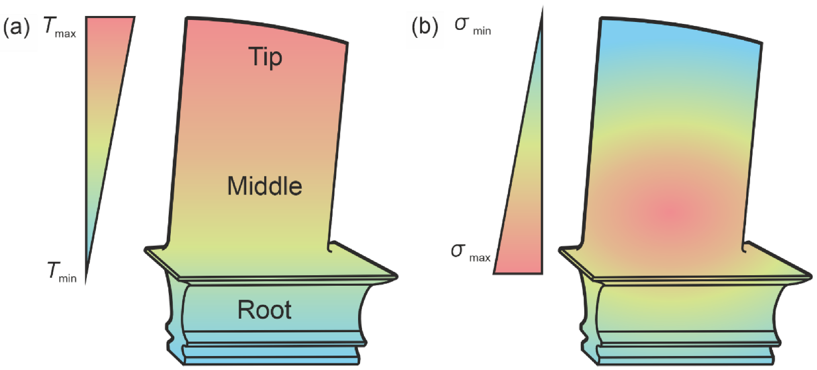
Schematic distribution of (a) temperature and (b) mechanical stress in a turbine blade.
Figure 1.
Schematic distribution of (a) temperature and (b) mechanical stress in a turbine blade.
Figure 2.
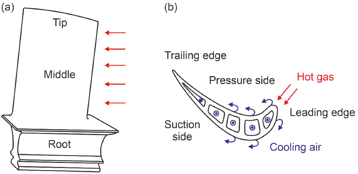
Schematic drawings of the ex-service blade investigated in the present study: (a) Front view and (b) top view. Blue arrows indicate cold air flow, while red arrows represent hot gas flow.
Figure 2.
Schematic drawings of the ex-service blade investigated in the present study: (a) Front view and (b) top view. Blue arrows indicate cold air flow, while red arrows represent hot gas flow.
Figure 3.
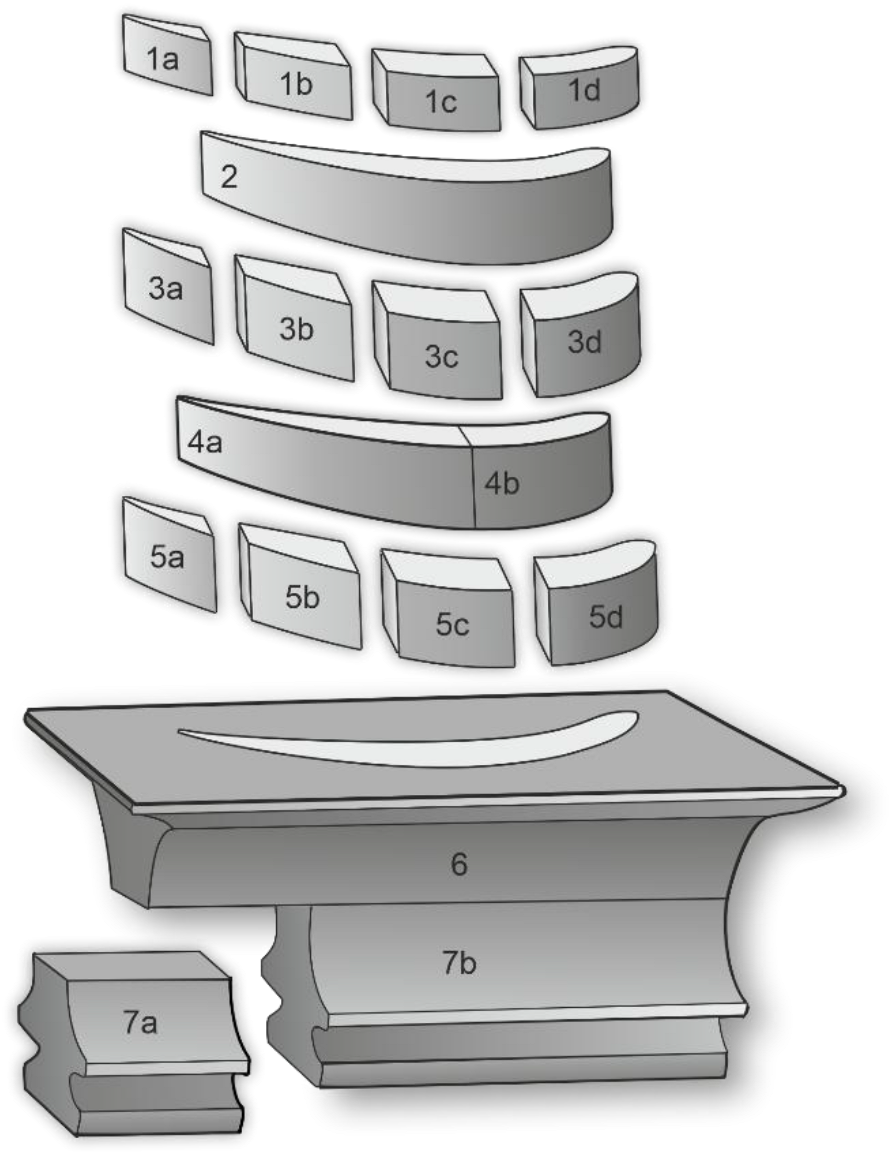
Numbering of individual blade locations after waterjet cutting.
Figure 3.
Numbering of individual blade locations after waterjet cutting.
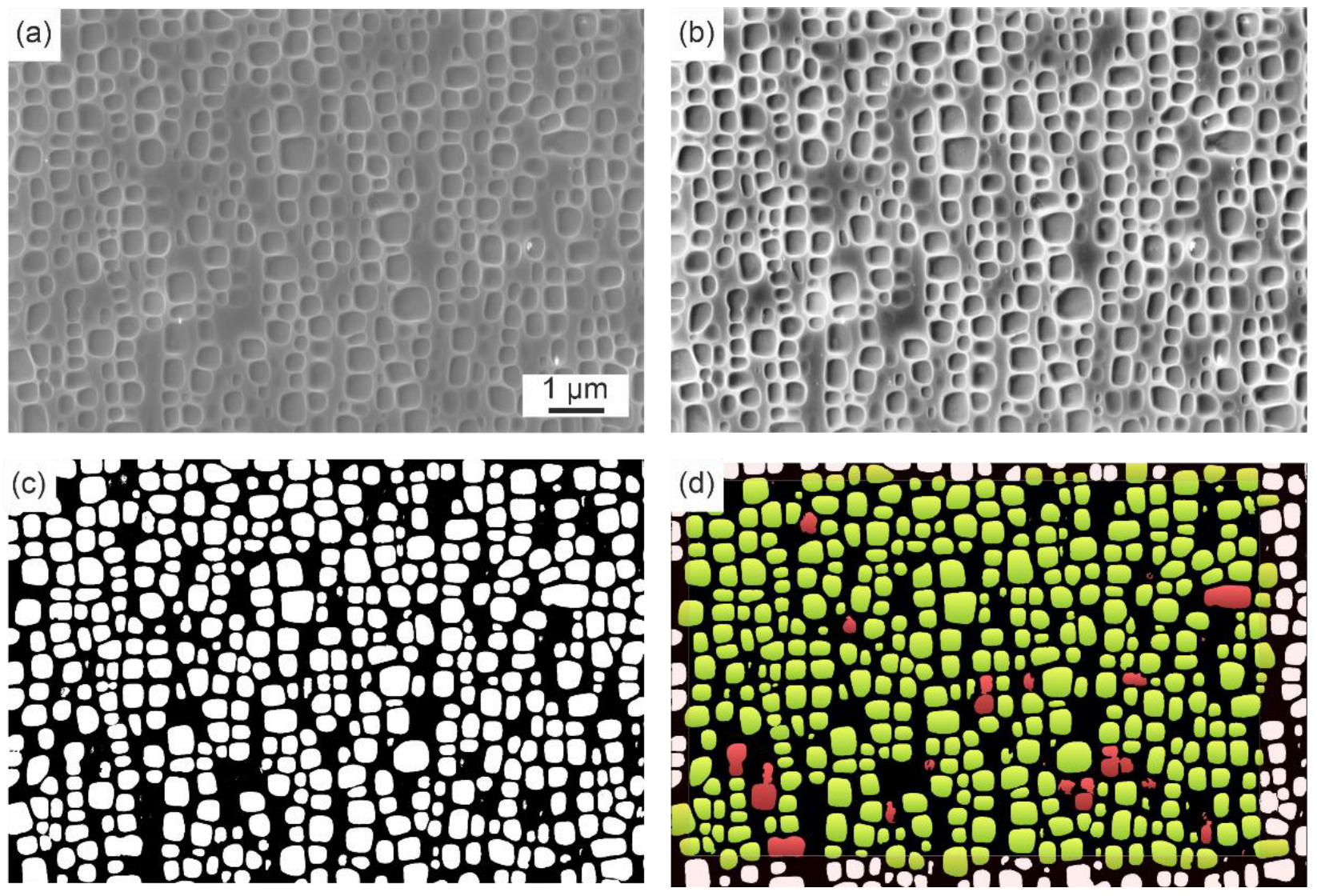
Figure 4.
Evaluation of SEM images. (a) Original image (tip region). (b) Image with improved grey level contrast. (c) Segmented image. (d) Green color-coded particles were used for analysis of particle sizes (horizontal and vertical Feret values). Incorrectly detected particles were manually excluded (red).
Figure 4.
Evaluation of SEM images. (a) Original image (tip region). (b) Image with improved grey level contrast. (c) Segmented image. (d) Green color-coded particles were used for analysis of particle sizes (horizontal and vertical Feret values). Incorrectly detected particles were manually excluded (red).
Figure 5.
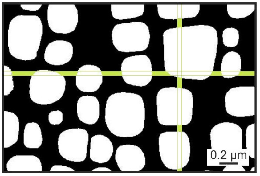
Schematic illustration of line intersection method which was used to determine the width of interparticle spacings.
Figure 5.
Schematic illustration of line intersection method which was used to determine the width of interparticle spacings.
Figure 6.
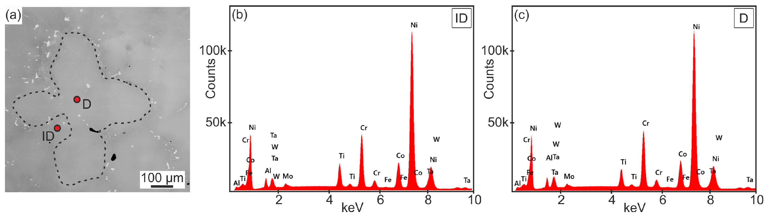
Examples of individual EDX spectra: (a) SEM micrograph (backscattered electron contrast) showing the selected measurement locations in the interdendritic (ID) and dendritic (D) regions. (b) EDX spectrum acquired from the ID at the blade tip (location 1a); (c) EDX spectrum acquired from the D at the blade root (location 7a).
Figure 6.
Examples of individual EDX spectra: (a) SEM micrograph (backscattered electron contrast) showing the selected measurement locations in the interdendritic (ID) and dendritic (D) regions. (b) EDX spectrum acquired from the ID at the blade tip (location 1a); (c) EDX spectrum acquired from the D at the blade root (location 7a).
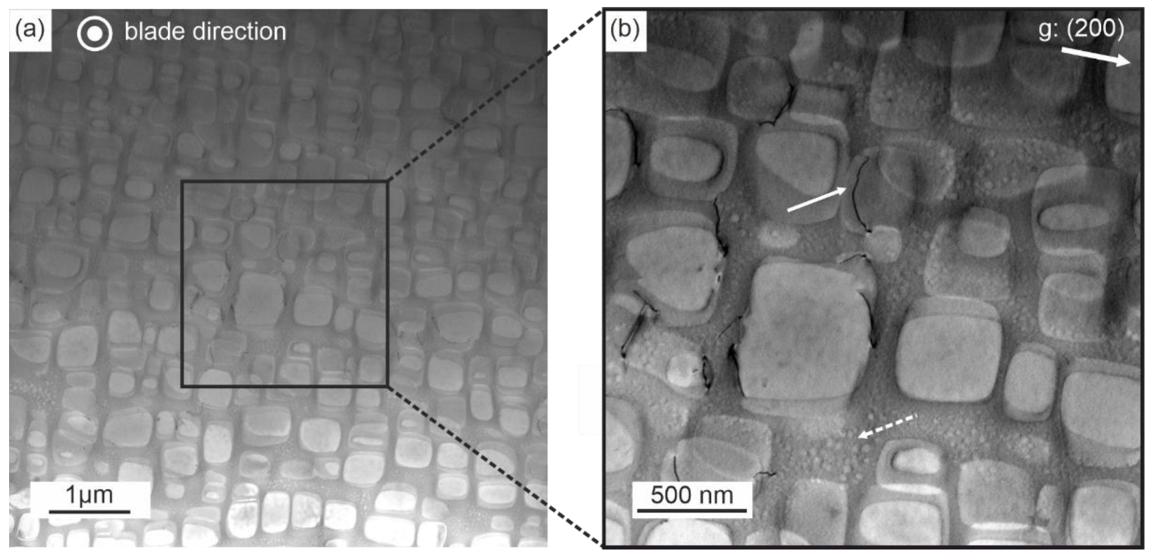
Figure 7.
(S)TEM micrographs taken from the root section of the blade (location 7a); g-vector and blade direction indicated. (a) Overview micrograph taken at a lower magnification. Blade direction indicated. (b) Higher magnification micrograph from region highlighted with a black rectangle in (a). g-vector indicated by the white arrow in the upper right corner.
Figure 7.
(S)TEM micrographs taken from the root section of the blade (location 7a); g-vector and blade direction indicated. (a) Overview micrograph taken at a lower magnification. Blade direction indicated. (b) Higher magnification micrograph from region highlighted with a black rectangle in (a). g-vector indicated by the white arrow in the upper right corner.
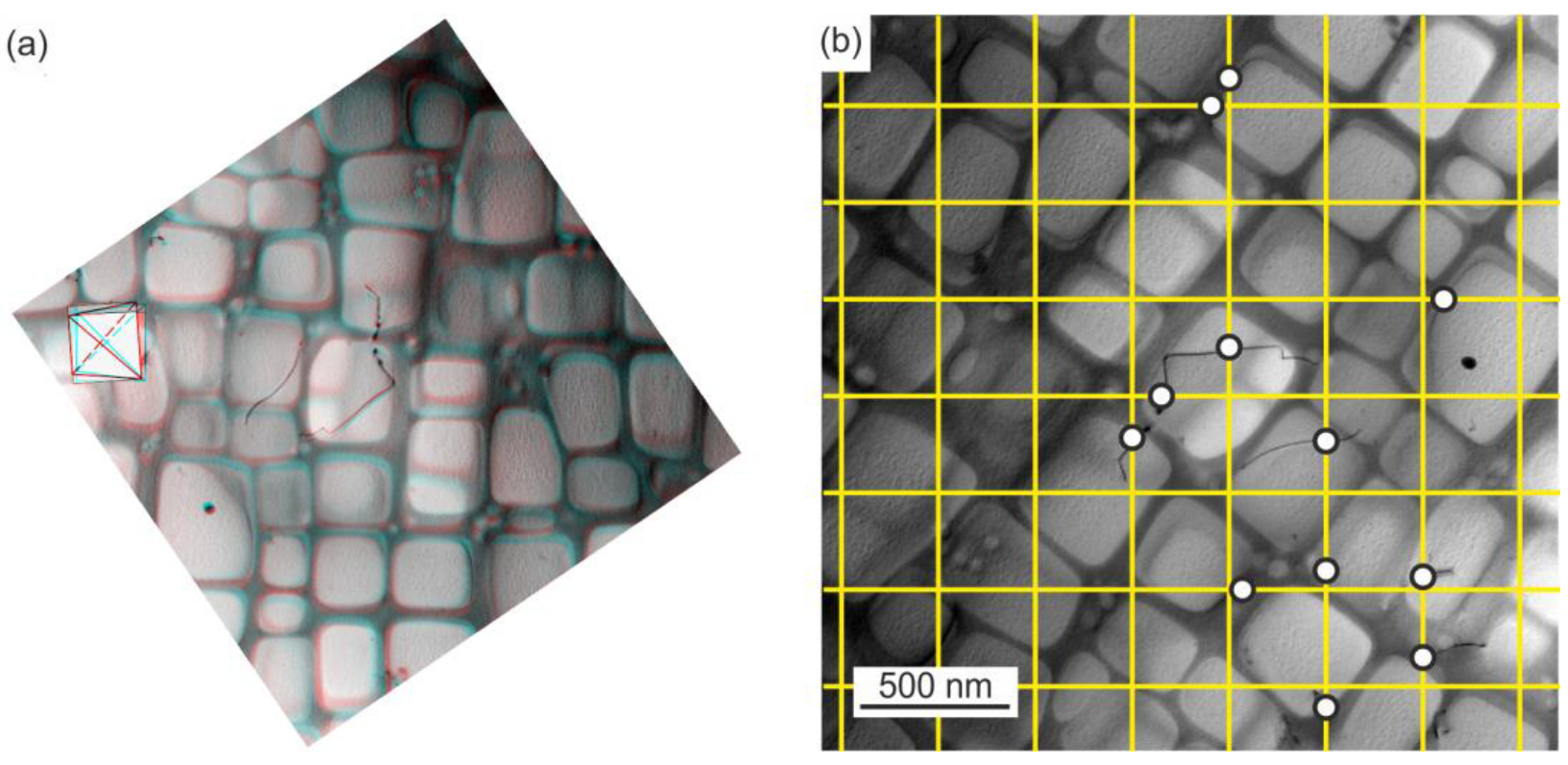
Figure 8.
(S)TEM micrographs illustrating the use of Ham’s method. (a) Stereo-(S)TEM image which was used for the determination of foil thickness. (b) Grid with reference lines and marked dislocation intersections used to determine dislocation densities.
Figure 8.
(S)TEM micrographs illustrating the use of Ham’s method. (a) Stereo-(S)TEM image which was used for the determination of foil thickness. (b) Grid with reference lines and marked dislocation intersections used to determine dislocation densities.
Figure 9.
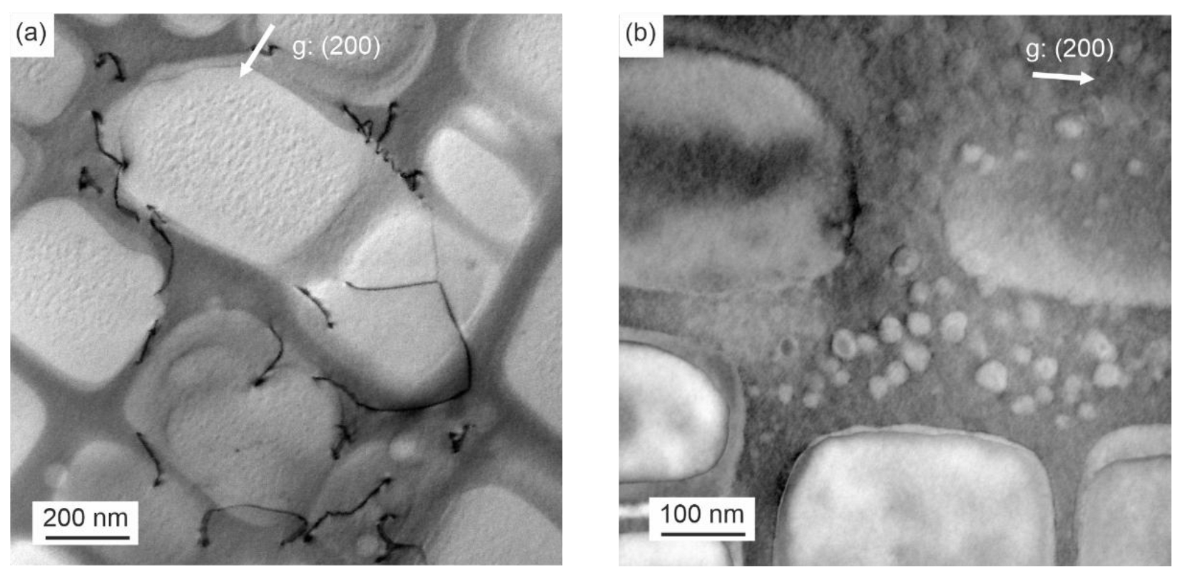
(S)TEM micrographs: (a) Dislocations in middle location. (b) Small tertiary particles in root location.
Figure 9.
(S)TEM micrographs: (a) Dislocations in middle location. (b) Small tertiary particles in root location.
Figure 10.
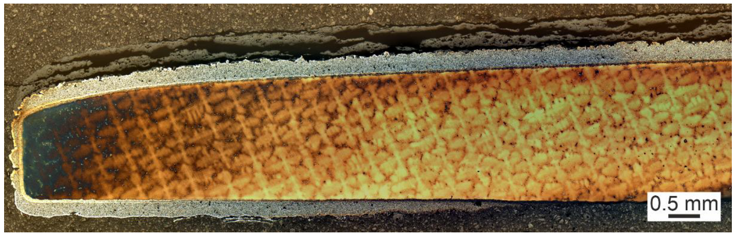
Optical micrograph of dendritic microstructure and the protective coating. The cross section was prepared from the bottom of blade piece 1a (view: in tip direction).
Figure 10.
Optical micrograph of dendritic microstructure and the protective coating. The cross section was prepared from the bottom of blade piece 1a (view: in tip direction).
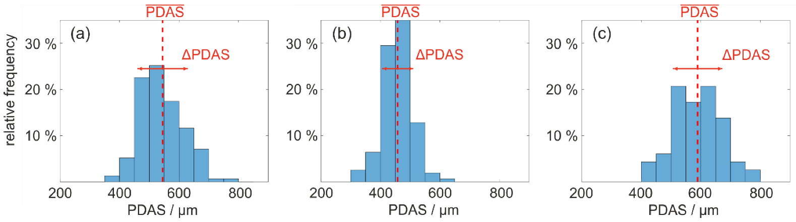
Figure 11.
Relative frequencies of primary dendrite spacings (PDAS) at different blade locations. (a) Root, location 7a. (b) Middle, location 5a. (c) Tip, location 1a. Average and the corresponding standard deviation ∆PDAS are indicated.
Figure 11.
Relative frequencies of primary dendrite spacings (PDAS) at different blade locations. (a) Root, location 7a. (b) Middle, location 5a. (c) Tip, location 1a. Average and the corresponding standard deviation ∆PDAS are indicated.
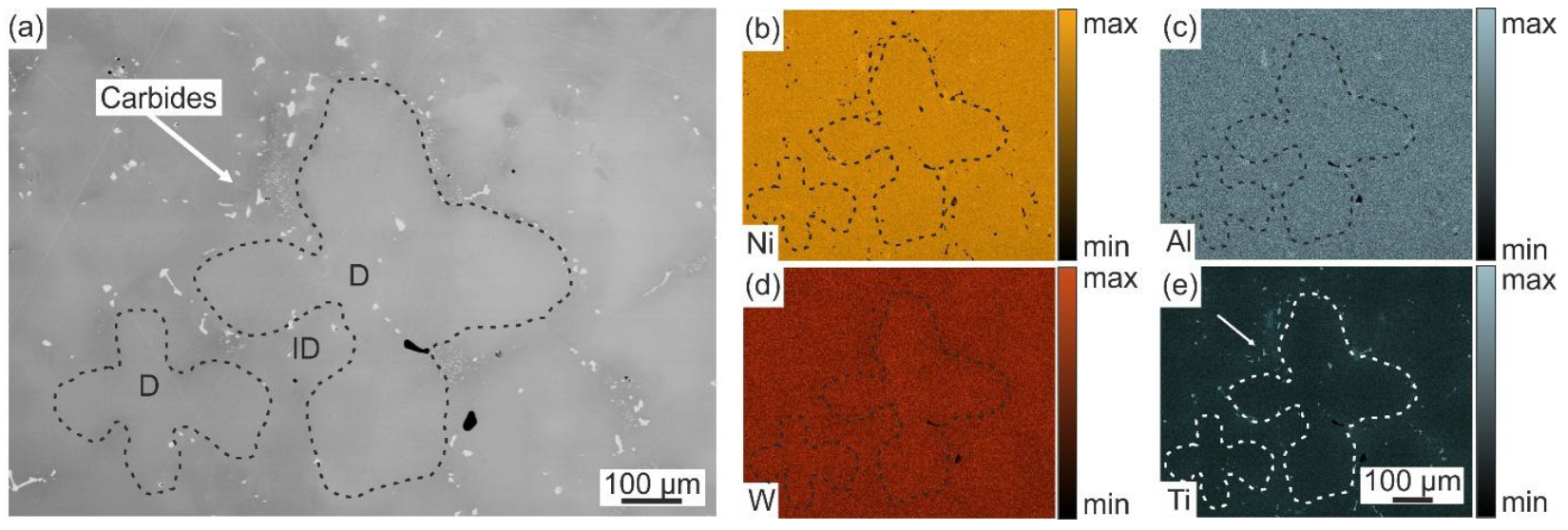
Figure 12.
Element distribution in dendritic and interdendritic regions (blade location 1a). (a) BSE-micrograph with dendritic and interdendritic regions. Two dendrites are highlighted by dashed lines. (b–e) Elemental distribution of Ni, Al, W and Ti.
Figure 12.
Element distribution in dendritic and interdendritic regions (blade location 1a). (a) BSE-micrograph with dendritic and interdendritic regions. Two dendrites are highlighted by dashed lines. (b–e) Elemental distribution of Ni, Al, W and Ti.
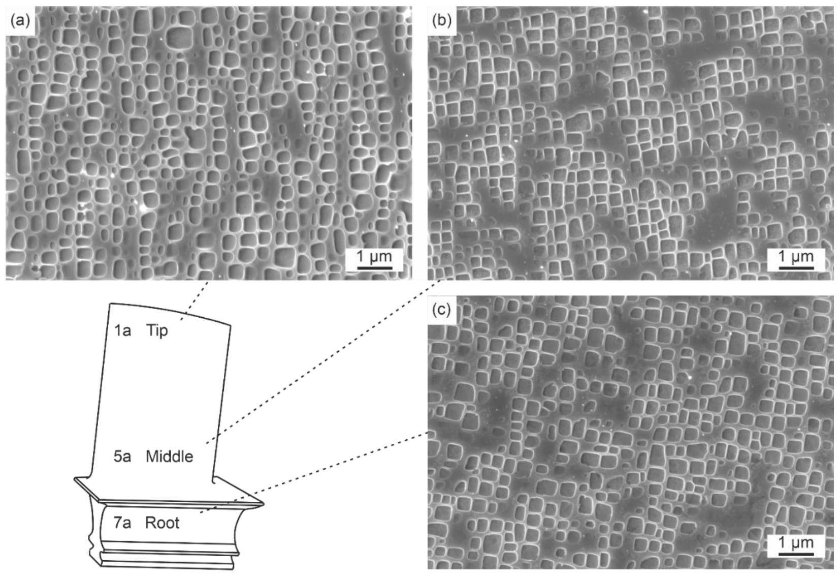
Figure 13.
SEM micrographs (SE contrast) of the γ/γ’-microstructure at different blade locations as indicated. (a) Tip, location 1a. (b) Middle, location 5a. (c) Root, location 7a.
Figure 13.
SEM micrographs (SE contrast) of the γ/γ’-microstructure at different blade locations as indicated. (a) Tip, location 1a. (b) Middle, location 5a. (c) Root, location 7a.
Figure 14.
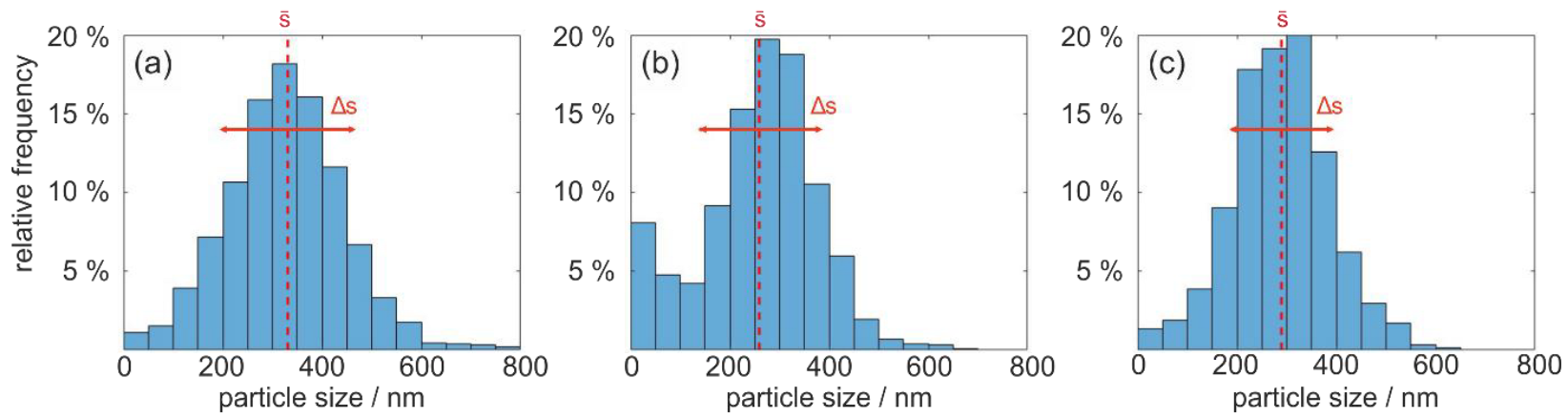
Histograms showing the relative frequency of particle sizes in 50 nm size classes at the three blade locations. (a) 1a (tip). (b) 5a (middle). (c) 7a (root). Average and the corresponding standard deviation ∆s are indicated.
Figure 14.
Histograms showing the relative frequency of particle sizes in 50 nm size classes at the three blade locations. (a) 1a (tip). (b) 5a (middle). (c) 7a (root). Average and the corresponding standard deviation ∆s are indicated.
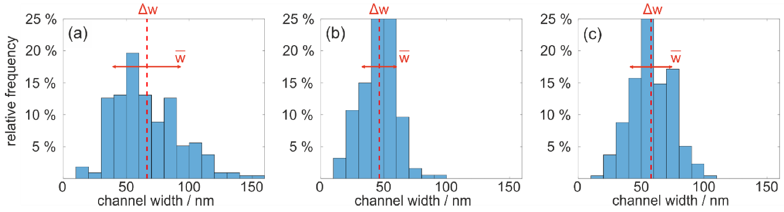
Figure 15.
Histograms showing the relative frequency of γ-channel widths attributed to 10 nm size classes for the three blade locations. (a) 1a (tip). (b) 5a (middle). (c) 7a (root). Average and the corresponding standard deviation ∆w are indicated.
Figure 15.
Histograms showing the relative frequency of γ-channel widths attributed to 10 nm size classes for the three blade locations. (a) 1a (tip). (b) 5a (middle). (c) 7a (root). Average and the corresponding standard deviation ∆w are indicated.
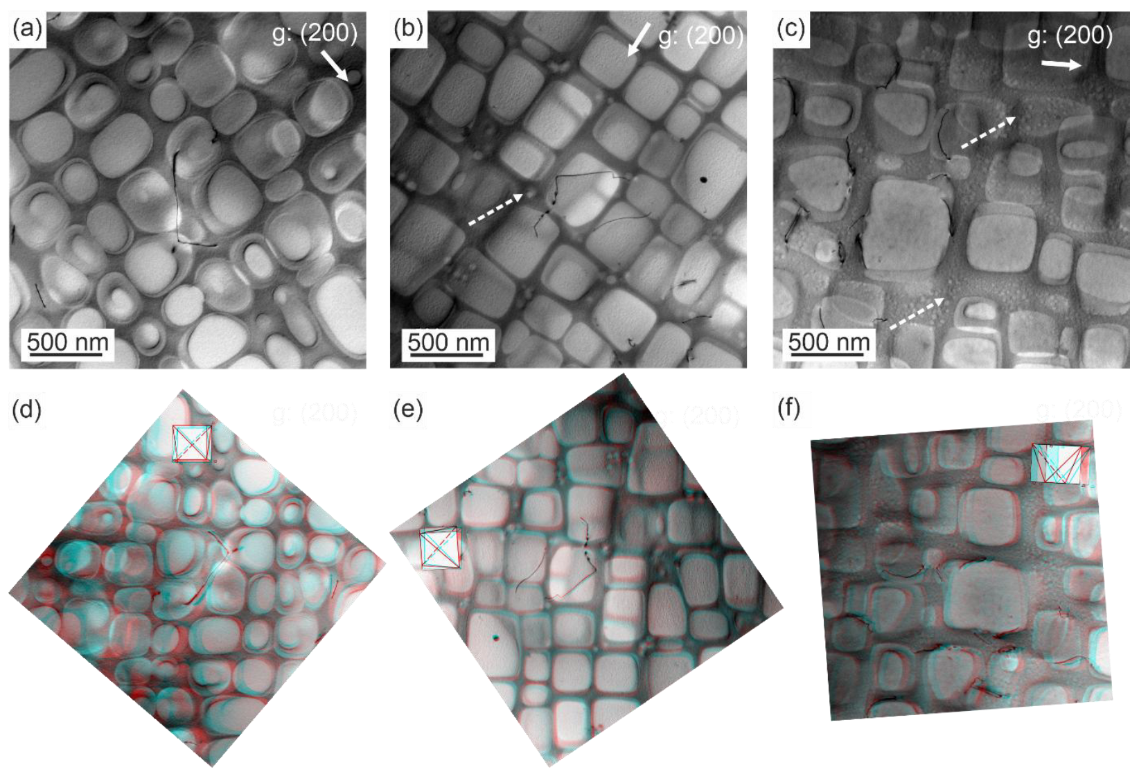
Figure 16.
(S)TEM images taken under g = (200) two-beam conditions as indicated. (
a–
c) (S)TEM micrographs. (
d–
f) 3D anaglyph obtained by the Agudo method [
29]. (
a,
d) Blade tip location 1a. (
b,
e) Middle location 5a. (
c,
f) Blade root location 7a. Tertiary particles are indicated by dashed white arrows.
Figure 16.
(S)TEM images taken under g = (200) two-beam conditions as indicated. (
a–
c) (S)TEM micrographs. (
d–
f) 3D anaglyph obtained by the Agudo method [
29]. (
a,
d) Blade tip location 1a. (
b,
e) Middle location 5a. (
c,
f) Blade root location 7a. Tertiary particles are indicated by dashed white arrows.
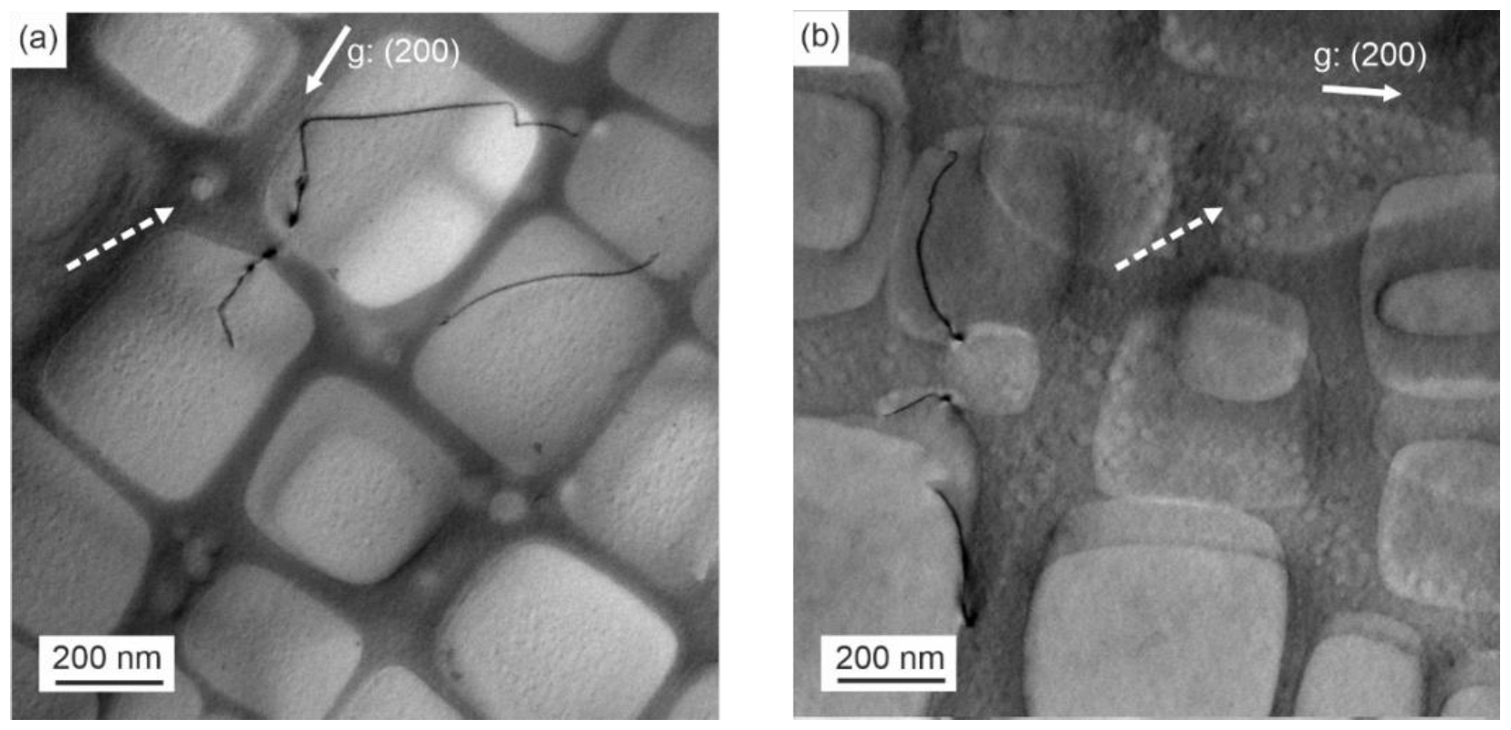
Figure 17.
(S)TEM micrographs. (a) Small tertiary particles in middle location. (b) Small tertiary particles in root location are indicated by dashed white arrows.
Figure 17.
(S)TEM micrographs. (a) Small tertiary particles in middle location. (b) Small tertiary particles in root location are indicated by dashed white arrows.
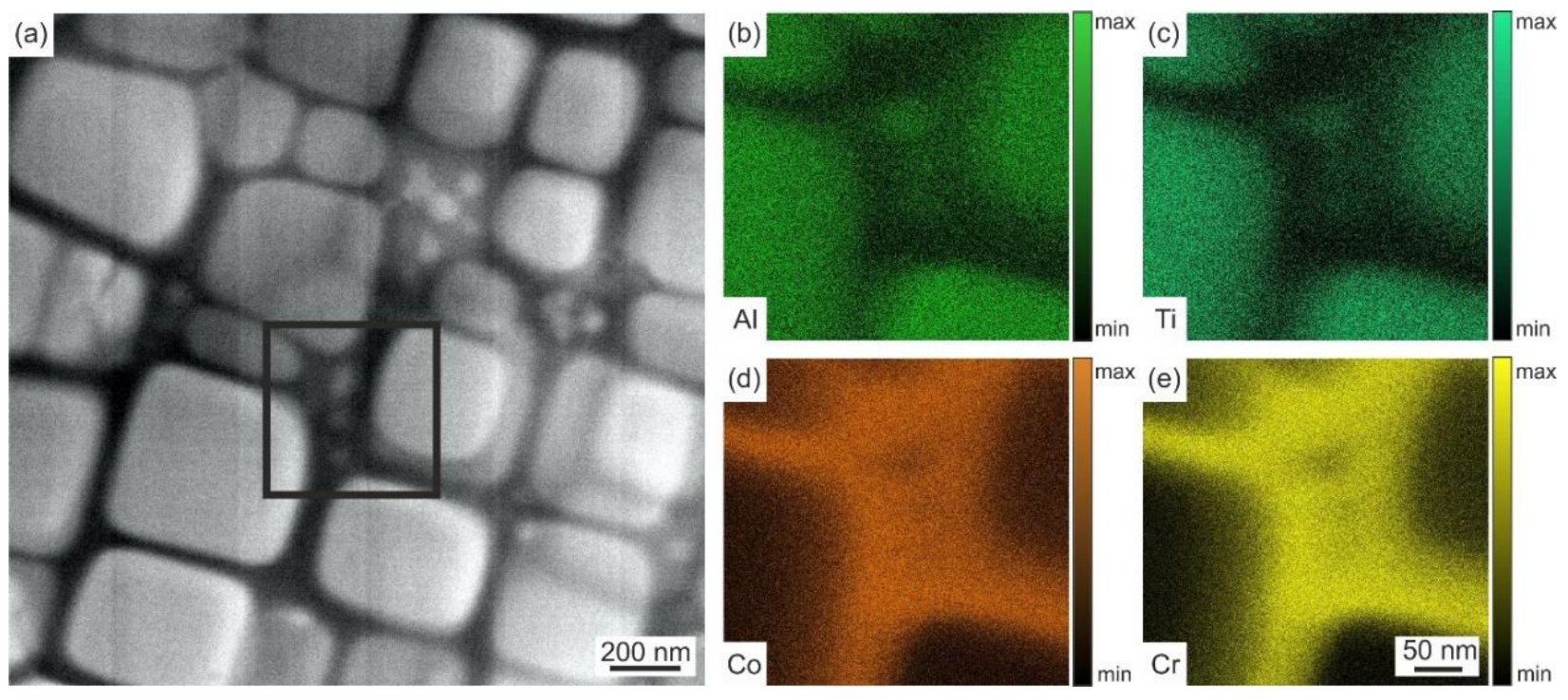
Figure 18.
STEM-EDX analysis of small tertiary γ’-particle. (a) AMAG-STEM image with marked region of interest (ROI). (b–e) Distribution of Al, Ti, Co and Cr from ROI. The small particles exhibit enrichment in Al and Ti and depletion in Co and Cr, like the larger cuboidal γ’-particles.
Figure 18.
STEM-EDX analysis of small tertiary γ’-particle. (a) AMAG-STEM image with marked region of interest (ROI). (b–e) Distribution of Al, Ti, Co and Cr from ROI. The small particles exhibit enrichment in Al and Ti and depletion in Co and Cr, like the larger cuboidal γ’-particles.
Table 1.
EDX results for Al from interdendritic region (ID) and W from dendritic region (D) from 5 point measurements for each element.
Table 1.
EDX results for Al from interdendritic region (ID) and W from dendritic region (D) from 5 point measurements for each element.
| Blade Location | Microstr. Region | Element | Concentration/wt.% |
|---|
| 1a | ID | Al | 3.2 |
| “ | “ | “ | 3.4 |
| “ | “ | “ | 3.8 |
| “ | “ | “ | 3.6 |
| “ | “ | “ | 3.6 |
| 7a | D | W | 4.5 |
| “ | “ | “ | 4.7 |
| “ | “ | “ | 4.7 |
| “ | “ | “ | 4.8 |
| “ | “ | “ | 4.7 |
Table 2.
Primary dendrite arm spacings at three blade locations.
Table 2.
Primary dendrite arm spacings at three blade locations.
| Blade Location | Number of Dendrites | Average PDAS/µm | ∆PDAS/µm |
|---|
| 1a | 155 | 545 | 82 |
| 5a | 156 | 432 | 47 |
| 7a | 116 | 589 | 81 |
Table 3.
Comparison of chemical composition (in wt.%) of interdendritic (ID) and dendritic (D) regions of the microstructure in different blade locations (1a and 7a). Mean value M and standard deviation ∆M were determined.
Table 3.
Comparison of chemical composition (in wt.%) of interdendritic (ID) and dendritic (D) regions of the microstructure in different blade locations (1a and 7a). Mean value M and standard deviation ∆M were determined.
| Blade Location | Region | Al | Co | Cr | Fe | Mo | Ta | Ti | W |
|---|
| 1a | ID | 3.7 | 8.4 | 11.5 | 0.3 | 1.6 | 7.9 | 4.5 | 3.2 |
| 7a | ID | 2.9 | 8.8 | 11.9 | 0.5 | 1.3 | 7.2 | 4.1 | 3.2 |
| 1a | D | 3.7 | 8.5 | 11.8 | 0.4 | 1.3 | 7.9 | 3.7 | 5.2 |
| 7a | D | 2.9 | 9.0 | 12.2 | 0.5 | 1.7 | 6.7 | 3.5 | 4.4 |
| M | – | 3.3 | 8.7 | 11.9 | 0.4 | 1.5 | 7.4 | 4.0 | 4.0 |
| ∆M | – | 0.4 | 0.2 | 0.2 | 0.1 | 0.2 | 0.5 | 0.4 | 0.8 |
Table 4.
Mean values and mean deviations from mean values of particle sizes as measured by SEM for the blade locations 1a, 5a and 7a. Area fractions fV and roundness parameters of particles R are also reported.
Table 4.
Mean values and mean deviations from mean values of particle sizes as measured by SEM for the blade locations 1a, 5a and 7a. Area fractions fV and roundness parameters of particles R are also reported.
| Blade Location | No. Particles | /nm | /nm | fV2nd/% | R |
|---|
| 1a | 1144 | 330 | 110 | 56 | 0.99 |
| 5a | 1317 | 259 | 117 | 61 | 0.96 |
| 7a | 1115 | 289 | 98 | 58 | 0.97 |
Table 5.
Mean values and mean deviations from mean values of channel widths as measured by SEM for the four blades segments (blade positions 1a, 5a and 7a).
Table 5.
Mean values and mean deviations from mean values of channel widths as measured by SEM for the four blades segments (blade positions 1a, 5a and 7a).
| Blade Location | No. of Channels | /nm | /nm
|
|---|
| 1a | 214 | 66 | 26 |
| 5a | 187 | 46 | 13 |
| 7a | 216 | 58 | 16 |
Table 6.
TEM evaluation of tertiary particles and correction of SEM-volume fractions. L—blade location, nP number of tertiary particles considered, d—average size of tertiary particles, VP—total volume of all tertiary particles, VT—size of test volume (Equation (4)), fV3rd—volume fraction of tertiary particles in % (Equation (5)), fV—final volume fraction (secondary and tertiary particles (Equation (6)).
Table 6.
TEM evaluation of tertiary particles and correction of SEM-volume fractions. L—blade location, nP number of tertiary particles considered, d—average size of tertiary particles, VP—total volume of all tertiary particles, VT—size of test volume (Equation (4)), fV3rd—volume fraction of tertiary particles in % (Equation (5)), fV—final volume fraction (secondary and tertiary particles (Equation (6)).
| L | nP | d/nm | VP/µm3 | VT/µm3 | fV3rd/% | fV/% |
|---|
| 5a | 118 | 46 ± 15 | 88 × 10−4 | 1.06 | 0.8 | 61.8 |
| 7a | 145 | 14 ± 9 | 3 × 10⁻⁴ | 0.06 | 0.6 | 58.6 |
Table 7.
Dislocation densities ρ evaluated from different blade locations 1a, 5a and 7a.
Table 7.
Dislocation densities ρ evaluated from different blade locations 1a, 5a and 7a.
| Location | Area/µm2 | Foil Thickness/µm | Eval. Volume/µm3 | ρ/1012m−2 |
|---|
| 1a | 49 | 0.14 | 6.8 | 3.7 |
| 5a | 49 | 0.18 | 8.7 | 4.3 |
| 7a | 49 | 0.13 | 6.3 | 1.9 |
Table 8.
Hardness (HV10) values at the three blade locations 1a, 5a and 7a.
Table 8.
Hardness (HV10) values at the three blade locations 1a, 5a and 7a.
| Location | 1a | 5a | 7a |
|---|
| HV10 | 430 ± 6 | 450 ± 6 | 420 ± 2 |




 ,
,