From the Variational Principle to the Legendre Transform: A Revisit of the Wulff Construction and Its Computational Realization

Abstract

The equilibrium shape of a crystal is a fundamental problem in materials science and condensed matter physics. The Wulff construction, a cornerstone of crystal morphology prediction, is traditionally presented and utilized as a powerful geometric algorithm to derive equilibrium shapes from anisotropic surface energy $\gamma \left(\mathbf{n}\right)$. While its application across materials science is vast, the profound mathematical physics underpinning it, specifically its intrinsic identity as a manifestation of the Legendre transform, is often relegated to a passing remark. This work recenters the focus on this fundamental duality. We present a comprehensive, step-by-step derivation of the Wulff shape from the variational principle of surface energy minimization under a constant volume, employing the language of support functions and differential geometry. We then rigorously demonstrate that the equilibrium shape, defined by the support function $h\left(\mathbf{n}\right)$, and the surface energy density $\gamma \left(\mathbf{n}\right)$ are conjugate variables linked by a Legendre transformation; the Wulff shape $\mathcal{W}$ is precisely the zero-sublevel set of the dual function ${\gamma }^{*}\left(\mathbf{x}\right)={sup}_{\mathbf{n}}[\mathbf{x}·\mathbf{n}-\gamma \left(\mathbf{n}\right)]$. This perspective elevates the Wulff construction from a mere graphical tool to a canonical example of convex duality in thermodynamic systems, connecting it to deeper principles in convex analysis and statistical mechanics. To bridge theory and computation, we provide a robust computational algorithm implemented in pseudocode capable of generating Wulff shapes for two-dimensional (2D) crystals with arbitrary N-fold symmetry. Finally, we discuss the relevance and extensions of the classical theory in contemporary research, including non-equilibrium growth, nanoscale effects, and the coupling of crystal shapes with elastic membrane environments.

1. Introduction

The equilibrium shape of a crystal, namely the manifestation of anisotropic interfacial tensions at thermodynamic equilibrium, has captivated scientists since the seminal work of Gibbs and Wulff. Wulff’s original construction gives a practical way to predict shapes [1], but working through its geometry often obscures why this particular algorithm solves the variational problem. Here, we find a deeper geometric structure. Given the orientation-dependent surface free energy $\gamma \left(\mathbf{n}\right)$, where $\mathbf{n}\in S^{d-1}$ is the outward normal unit, the equilibrium shape $\mathcal{W}$ is the convex set defined by the intersection of half-spaces:

$$\mathcal{W}=\bigcap _{\mathbf{n}\in S^{d-1}}\{\mathbf{x}\in {\mathbb{R}}^d:\mathbf{x}·\mathbf{n}\le \gamma \left(\mathbf{n}\right)\}.$$

(1)

This construction is the visual solution to the Gibbs–Curie–Wulff variational principle, which states that the equilibrium shape minimizes the total surface energy $E_{\mathrm{surf}}={\int }_{\partial \mathcal{W}}\gamma \left(\mathbf{n}\right)dS$ for a fixed enclosed volume V.

The utility of the Wulff construction as an application tool is undeniable and forms the focus of a vast body of research [2,3,4,5,6,7,8,9,10,11]. It is the standard method for predicting nanoparticle morphologies from first-principle surface energy calculations [12,13] for analyzing the equilibrium shape of thin films and supported clusters via the Wulff–Kaishew theorem [6] and for interpreting experimental observations from techniques like low-energy electron microscopy (LEEM) [3]. This applied focus is perfectly natural and has driven significant progress in materials design. Recent comprehensive reviews on crystal morphology prediction models and regulating strategies further underscore the central role of the Wulff construction in modern materials design [14].

However, this widespread application-centric narrative has, perhaps inadvertently, obscured a deeper and more elegant mathematical reality. As noted in several theoretical works, “the equilibrium shape function is the Legendre transform of $\gamma \left(\mathbf{n}\right)$ and vice versa” [3,15]. This statement points to a fundamental duality that transcends the specific geometric algorithm of drawing perpendicular planes. The Wulff shape is not merely the output of a minimization procedure; it is the geometric realization of the convex conjugate of the surface energy function. The support function $h\left(\mathbf{n}\right)={max}_{\mathbf{x}\in \mathcal{W}}\mathbf{x}·\mathbf{n}$ of the equilibrium crystal and the surface energy $\gamma \left(\mathbf{n}\right)$ are conjugate variables in the sense of Legendre–Fenchel transformation. This duality, while acknowledged, is frequently presented as a curious mathematical footnote rather than the central organizing principle it truly is. Its detailed exposition, from first variational principles to the explicit identification of the Legendre pair, is often abbreviated or omitted in favor of the more intuitive geometric construction. This gap in pedagogical and conceptual clarity is what the present work aims to address.

Our primary objective is a systematic and detailed exposition that re-establishes the Legendre transform as the foundational core of the Wulff construction. We aim to demonstrate that the variational derivation naturally and inevitably leads to this duality. The journey from the energy functional $E_{\mathrm{surf}}\left[h\right]$ to the proportionality condition $h\left(\mathbf{n}\right)\propto \gamma \left(\mathbf{n}\right)$ is, in essence, the process of constructing the Legendre transform. This perspective unifies the Wulff problem with a broad landscape of convex analysis and thermodynamic potential theory, offering a more powerful lens through which to view not only equilibrium shapes but also potential generalizations, such as elastic solid-phase membrane domains in fluid vesicles [16,17] and elastic monolayer domains in the air–water interface [18], which both involve interfacial interactions. Moreover, we have found that charged elastic solid crystals can trigger the exotic intrinsic phase transition [19,20], and the active Janus particles can arrange more complicated crystalline shapes [21]. All the recent findings urge us to find a deeper and new understanding of the traditional theoretical tool known as the Wulff construction.

The structure of this paper is as follows. In Section 2, we lay the geometric groundwork by introducing the support function parameterization of convex bodies. We then carefully derive expressions for the surface area and volume in terms of the support function $h\left(\mathbf{n}\right)$ and its curvature-related derivatives. The constrained variational problem is set up and solved in detail, leading to the Wulff proportionality condition. Section 3 is the conceptual heart of the paper. We review the definition of the Legendre transform for positively homogeneous functions and prove that the Wulff set $\mathcal{W}$ is exactly the zero-sublevel set of the transform ${\gamma }^{*}\left(\mathbf{x}\right)$. We trace the path from the variational solution to this identification, highlighting the role of convex duality. The algorithm in Section 4 is a natural application and implementation of the preceding theory. It transforms the abstract mathematical derivations (variational principles and Legendre transforms) into concrete computational steps, allowing us to visualize and verify the Wulff shape numerically. Section 5 discusses the implications of this viewpoint, connecting it to concepts in statistical mechanics (surface tension and large deviations) and hinting at extensions beyond the classical equilibrium setting. We conclude and provide perspective in Section 6.

2. Variational Derivation: From Energy Minimization to the Wulff Condition

2.1. Geometry of Convex Bodies and the Support Function

Let $\mathcal{K}\subset {\mathbb{R}}^d$ be a compact convex body containing the origin in its interior. Its shape can be completely described by the support function $h_{\mathcal{K}}:S^{d-1}\to \mathbb{R}$, defined as

$$h\left(\mathbf{n}\right)=h_{\mathcal{K}}\left(\mathbf{n}\right)=\underset{\mathbf{x}\in \mathcal{K}}{max}\mathbf{x}·\mathbf{n}.$$

(2)

Geometrically, $h\left(\mathbf{n}\right)$ is the signed distance from the origin to the supporting hyperplane of $\mathcal{K}$ with the outward normal unit $\mathbf{n}$. The boundary $\partial \mathcal{K}$ is given by the set of points $\mathbf{x}$ such that $\mathbf{x}·\mathbf{n}=h\left(\mathbf{n}\right)$ for the appropriate $\mathbf{n}$.

For a smooth, strictly convex body, the mapping between a boundary point $\mathbf{x}$ and its unique outer normal $\mathbf{n}$ is one-to-one. In this case, we can parameterize the boundary with $\mathbf{n}\in S^{d-1}$. The position vector $\mathbf{x}\left(\mathbf{n}\right)$ of the point with the normal $\mathbf{n}$ satisfies

$$\mathbf{x}\left(\mathbf{n}\right)=h\left(\mathbf{n}\right)\mathbf{n}+{\nabla }_{S}h\left(\mathbf{n}\right),$$

(3)

where ${\nabla }_S$ denotes the gradient on the unit sphere $S^{d-1}$. This follows from the fact that $\mathbf{x}$ must be the point maximizing $\mathbf{x}·\mathbf{n}$ for the given $\mathbf{n}$, and the tangential component arises from the derivative of this condition.

2.2. Surface Area and Volume in Terms of $h\left(\mathbf{n}\right)$

To express the total surface energy as a functional of h, we need the surface area element $dS$ on $\partial \mathcal{K}$ in terms of h and its derivatives. The relevant quantity is the Hessian of h on the sphere. Let $g_{ij}$ be the standard metric on $S^{d-1}$ (e.g., in spherical coordinates). We define the second fundamental form tensor as follows:

$$h_{ij}={\nabla }_i{\nabla }_{j}h+h{g}_{ij},$$

(4)

where ${\nabla }_i$ denotes the covariant derivative on $S^{d-1}$. For a convex body, $h_{ij}$ is a positive-definite symmetric tensor. Its determinant is related to the Gaussian curvature $K\left(\mathbf{n}\right)$ of the surface at the point with the normal $\mathbf{n}$.

A fundamental result from convex geometry states that the surface area measured on $\partial \mathcal{K}$ induced by the spherical map is

$$dS=\sqrt{det\left(h_{ij}\right)}d\Omega ,$$

(5)

where $d\Omega$ is the standard volume element (solid angle) on $S^{d-1}$. This can be understood by considering the Jacobian of the map from the spherical parameter domain to the surface.

The volume V of the convex body can also be expressed elegantly in terms of the support function. Using the divergence theorem or a direct geometric decomposition into cones from the origin, one obtains

$$V={\displaystyle \frac{1}{d}}{\int }_{S^{d-1}}h\left(\mathbf{n}\right)dS={\displaystyle \frac{1}{d}}{\int }_{S^{d-1}}h\left(\mathbf{n}\right)\sqrt{det\left(h_{ij}\right)}d\Omega .$$

(6)

For $d=2$, if we parameterize via $\theta$ with $\mathbf{n}=(cos\theta ,sin\theta )$, then $h_{ij}$ reduces to the scalar $h_{\theta \theta }+h$, and $\sqrt{det}=h+h_{\theta \theta }$. Thus, $dS=(h+h_{\theta \theta })d\theta$ and $V={\displaystyle \frac{1}{2}}{\int }_0^{2\pi }h(h+h_{\theta \theta })d\theta$, consistent with the known formulas.

2.3. The Variational Problem and Euler–Lagrange Equation

The total surface energy for a shape with a support function h is

$$E_{\mathrm{surf}}\left[h\right]={\int }_{S^{d-1}}\gamma \left(\mathbf{n}\right)dS={\int }_{S^{d-1}}\gamma \left(\mathbf{n}\right)\sqrt{det\left(h_{ij}\right)}d\Omega .$$

(7)

The equilibrium shape at a fixed volume $V_0$ is the minimizer of $E_{\mathrm{surf}}$, subject to the constraint $V\left[h\right]=V_0$. We introduce a Lagrange multiplier $\lambda$ and consider the functional

$$\mathcal{F}\left[h\right]=E_{\mathrm{surf}}\left[h\right]-\lambda (V\left[h\right]-V_0)={\int }_{S^{d-1}}\left[\gamma \left(\mathbf{n}\right)-{\displaystyle \frac{\lambda }{d}}h\left(\mathbf{n}\right)\right]\sqrt{det\left(h_{ij}\right)}d\Omega +\lambda V_0.$$

(8)

We seek the first variation $\delta \mathcal{F}=0$ for arbitrary variations $\delta h\left(\mathbf{n}\right)$ that preserve convexity. The variation of $\sqrt{det\left(h_{ij}\right)}$ is a standard result in differential geometry:

$$\delta \sqrt{det\left(h_{ij}\right)}=\sqrt{det\left(h_{ij}\right)}{\left(h^{-1}\right)}^{ij}\delta h_{ij},$$

(9)

where ${\left(h^{-1}\right)}^{ij}$ is the inverse tensor of $h_{ij}$ and $\delta h_{ij}={\nabla }_i{\nabla }_j\left(\delta h\right)+\left(\delta h\right)g_{ij}$.

Therefore, the variation of $\mathcal{F}$ is

$$\begin{array}{cc}\hfill \delta \mathcal{F}& ={\int }_{S^{d-1}}\left\{\left[\gamma \left(\mathbf{n}\right)-{\displaystyle \frac{\lambda }{d}}h\right]\delta \left(\sqrt{det}\right)-{\displaystyle \frac{\lambda }{d}}\delta h\sqrt{det}\right\}d\Omega \hfill \\ \hfill & ={\int }_{S^{d-1}}\left\{\left[\gamma -{\displaystyle \frac{\lambda }{d}}h\right]\sqrt{det}{\left(h^{-1}\right)}^{ij}\left({\nabla }_i{\nabla }_j\left(\delta h\right)+g_{ij}\delta h\right)-{\displaystyle \frac{\lambda }{d}}\delta h\sqrt{det}\right\}d\Omega .\hfill \end{array}$$

(10)

Let $H^{ij}=\sqrt{det}{\left(h^{-1}\right)}^{ij}$. Note that ${\left(h^{-1}\right)}^{ij}{g}_{ij}=\mathrm{Tr}\left(h^{-1}\right)$, which is related to the mean curvature. By integrating the term with ${\nabla }_i{\nabla }_j\left(\delta h\right)$ with parts twice over the closed manifold $S^{d-1}$ (where boundary terms vanish) and using the symmetry of $H^{ij}$, we can shift the derivatives onto $H^{ij}$

$$\begin{array}{cc}\hfill \int \left[\gamma -{\displaystyle \frac{\lambda }{d}}h\right]H^{ij}{\nabla }_i{\nabla }_j\left(\delta h\right)d\Omega & =\int {\nabla }_j\left(\left[\gamma -{\displaystyle \frac{\lambda }{d}}h\right]H^{ij}{\nabla }_i\left(\delta h\right)\right)d\Omega \hfill \\ \hfill & -\int {\nabla }_j\left(\left[\gamma -{\displaystyle \frac{\lambda }{d}}h\right]H^{ij}\right){\nabla }_i\left(\delta h\right)d\Omega \hfill \\ \hfill & =\int {\nabla }_i\left({\nabla }_j\left(\left[\gamma -{\displaystyle \frac{\lambda }{d}}h\right]H^{ij}\right)\right)\delta hd\Omega .\hfill \end{array}$$

(11)

The first term after the first equality is a total divergence and integrates to zero. The final expression is obtained by integrating via parts once more. When combining all terms, the variation becomes

$$\delta \mathcal{F}={\int }_{S^{d-1}}\left\{{\nabla }_i{\nabla }_j\left(\left[\gamma -{\displaystyle \frac{\lambda }{d}}h\right]H^{ij}\right)+\left[\gamma -{\displaystyle \frac{\lambda }{d}}h\right]H^{ij}{g}_{ij}-{\displaystyle \frac{\lambda }{d}}\sqrt{det}\right\}\delta hd\Omega .$$

(12)

For $\delta \mathcal{F}=0$ to hold for all smooth $\delta h$, the integrand must vanish pointwise. This yields a complex Euler–Lagrange partial differential equation. However, there is a celebrated special solution that satisfies a much simpler condition: the quantity in brackets before $H^{ij}$ is constant; that is, we have

$$\gamma \left(\mathbf{n}\right)-{\displaystyle \frac{\lambda }{d}}h\left(\mathbf{n}\right)=\mathrm{constant}.$$

(13)

Indeed, if this holds, then the derivatives in the first term vanish, and the remaining terms combine to give zero when the constant is chosen appropriately (often zero by redefining the origin or the multiplier). The constant can be absorbed into a redefinition of $\lambda$ or by observing that translating the shape adds the term t · n to h(n). This t-dependent linear term can be eliminated by redefining the origin (i.e., choosing the coordinate system such that t = 0) or absorbed into the Lagrange multiplier in the variational formulation when combined with the volume constraint. The key point is that the shape itself is invariant under translation, and the proportionality h(n) ∝ γ(n) is determined up to such a linear term, which is fixed by the condition that the origin is chosen appropriately (e.g., at the center of mass). Thus, the equilibrium condition reduces to the **Wulff proportionality**:

$$h\left(\mathbf{n}\right)={\displaystyle \frac{d}{\lambda }}\gamma \left(\mathbf{n}\right).$$

(14)

The Lagrange multiplier $\lambda$ is determined by substituting this relation into the volume constraint $V\left[h\right]=V_0$. Since both V and $E_{\mathrm{surf}}$ are homogeneous functionals, one finds $\lambda =d{E}_{\mathrm{surf}}/V_0$. Crucially, the shape itself is determined by the proportionality between h and $\gamma$ and not the absolute scale. Therefore, the equilibrium shape $\mathcal{W}$ is the set of points satisfying

$$\mathbf{x}·\mathbf{n}\le \gamma \left(\mathbf{n}\right)\mathrm{for}\mathrm{all}\mathbf{n},$$

(15)

which is exactly the classical Wulff construction of Equation (1). This completes the variational derivation. A detailed step-by-step algebraic derivation of this variational principle in two dimensions, including the handling of boundary terms and the explicit Euler–Lagrange equation, is presented in Appendix A. The variational calculus presented here for the classical Wulff problem aligns with the rigorous treatment of the first variation for more general functional Wulff shapes in modern convex geometry [22].

3. The Legendre Duality Underlying the Wulff Construction

3.1. Legendre–Fenchel Transform for Homogeneous Functions

Consider a continuous function $\gamma :S^{d-1}\to {\mathbb{R}}^{+}$. We can extend it to a positively homogeneous function with a degree of one on all of ${\mathbb{R}}^d\setminus \left\{0\right\}$ by defining

$$\Gamma \left(\mathbf{p}\right)=\left|\mathbf{p}\right|\gamma \left({\displaystyle \frac{\mathbf{p}}{\left|\mathbf{p}\right|}}\right),\mathrm{for}\mathbf{p}\ne 0.$$

(16)

This $\Gamma$ satisfies $\Gamma \left(t\mathbf{p}\right)=\left|t\right|\Gamma \left(\mathbf{p}\right)$ for $t\in \mathbb{R}$.

The Legendre–Fenchel transform (or convex conjugate) of $\Gamma$ is defined as follows:

$${\Gamma }^{*}\left(\mathbf{x}\right)=\underset{\mathbf{p}\in {\mathbb{R}}^d}{sup}\left\{\mathbf{x}·\mathbf{p}-\Gamma \left(\mathbf{p}\right)\right\}.$$

(17)

Due to the homogeneity of $\Gamma$, the supremum can be restricted to vectors $\mathbf{p}$ of a unit length. Let $\mathbf{p}=r\mathbf{n}$ with $r>0$ and $\mathbf{n}\in S^{d-1}$. Then, we have

$$\begin{array}{cc}\hfill {\Gamma }^{*}\left(\mathbf{x}\right)& =\underset{r>0,\mathbf{n}\in S^{d-1}}{sup}\left\{r(\mathbf{x}·\mathbf{n})-r\gamma \left(\mathbf{n}\right)\right\}\hfill \\ \hfill & =\underset{\mathbf{n}\in S^{d-1}}{sup}\left\{\underset{r>0}{sup}\left[r(\mathbf{x}·\mathbf{n}-\gamma (\mathbf{n}\left)\right)\right]\right\}.\hfill \end{array}$$

(18)

For a fixed $\mathbf{n}$, the inner supremum over r is

$$\underset{r>0}{sup}\left[r(\mathbf{x}·\mathbf{n}-\gamma (\mathbf{n}\left)\right)\right]=\left\{\begin{array}{cc}0\hfill & \mathrm{if}\mathbf{x}·\mathbf{n}-\gamma \left(\mathbf{n}\right)\le 0,\hfill \\ +\infty \hfill & \mathrm{if}\mathbf{x}·\mathbf{n}-\gamma \left(\mathbf{n}\right)>0.\hfill \end{array}\right.$$

Therefore, the overall supremum is finite (and equal to zero) if and only if $\mathbf{x}·\mathbf{n}\le \gamma \left(\mathbf{n}\right)$ for every $\mathbf{n}\in S^{d-1}$. If this condition is violated for even one $\mathbf{n}$, then the supremum is $+\infty$. Consequently, we have the elegant characterization

$${\Gamma }^{*}\left(\mathbf{x}\right)={\gamma }^{*}\left(\mathbf{x}\right)=\left\{\begin{array}{cc}0\hfill & \mathrm{if}\mathbf{x}\in \mathcal{W},\hfill \\ +\infty \hfill & \mathrm{if}\mathbf{x}\notin \mathcal{W},\hfill \end{array}\right.$$

(19)

where $\mathcal{W}$ is precisely the Wulff set defined in Equation (1). This is a powerful result, as the convex conjugate of the homogeneous surface energy function is the indicator function of the Wulff shape. The profound connection between anisotropic surface tension and equilibrium shape via convex duality has been recognized in the statistical physics literature for decades [23].

3.2. Equivalence of the Variational Solution and the Legendre Condition

We now connect this transform to the variational solution $h\left(\mathbf{n}\right)={\displaystyle \frac{d}{\lambda }}\gamma \left(\mathbf{n}\right)$. The support function $h\left(\mathbf{n}\right)$ of the Wulff shape $\mathcal{W}$ is, by definition, $h\left(\mathbf{n}\right)={max}_{\mathbf{x}\in \mathcal{W}}\mathbf{x}·\mathbf{n}$. Since $\mathcal{W}=\{\mathbf{x}:\mathbf{x}·\mathbf{m}\le \gamma (\mathbf{m})\forall \mathbf{m}\}$, we can write

$$h\left(\mathbf{n}\right)=\underset{\mathbf{x}}{max}\left\{\mathbf{x}·\mathbf{n}:\mathbf{x}·\mathbf{m}\le \gamma \left(\mathbf{m}\right)\forall \mathbf{m}\right\}.$$

(20)

which is a linear program. Its dual problem (in the sense of convex optimization) is to minimize ${\sum }_{\mathbf{m}}\gamma \left(\mathbf{m}\right)\mu \left(\mathbf{m}\right)$ over measures $\mu$, subject to ${\sum }_{\mathbf{m}}\mathbf{m}\mu \left(\mathbf{m}\right)=\mathbf{n}$ and $\mu \ge 0$. For a smooth $\gamma$, the optimal measure concentrates on a single $\mathbf{m}$, and the solution is given by the condition that $\mathbf{n}$ is proportional to the subgradient of $\gamma$ at $\mathbf{m}$, leading back to the proportionality of h and $\gamma$.

More directly, the very definition of the Legendre transform provides an alternative formula for the support function. Since $\mathcal{W}=\{\mathbf{x}:{\gamma }^{*}\left(\mathbf{x}\right)\le 0\}$, and ${\gamma }^{*}$ is the conjugate of $\Gamma$, we have under the biconjugation theorem (for convex $\Gamma$)

$$\Gamma \left(\mathbf{p}\right)=\underset{\mathbf{x}\in \mathcal{W}}{sup}\left\{\mathbf{x}·\mathbf{p}\right\}=h_{\mathcal{W}}\left(\mathbf{p}\right),$$

(21)

where the last equality holds because the supremum over $\mathcal{W}$ of a linear function defines the support function. However, $\Gamma \left(\mathbf{p}\right)=\left|\mathbf{p}\right|\gamma (\mathbf{p}/|\mathbf{p}\left|\right)$. For a unit vector $\mathbf{n}$, this gives

$$\gamma \left(\mathbf{n}\right)=\underset{\mathbf{x}\in \mathcal{W}}{sup}\mathbf{x}·\mathbf{n}=h_{\mathcal{W}}\left(\mathbf{n}\right).$$

(22)

which is the **inverse Wulff construction**, where the surface energy $\gamma \left(\mathbf{n}\right)$ is the support function of the Wulff shape $\mathcal{W}$. This is the complete duality: $\gamma$ and the indicator function of $\mathcal{W}$ are Legendre conjugates. In the context of the variational problem with a fixed volume, the scaling factor ${\displaystyle \frac{d}{\lambda }}$ appears, but it does not alter the essential duality between the functional forms of h and $\gamma$. The variational principle selects the specific scaled version of $\mathcal{W}$ whose volume is $V_0$, but the shape’s proportionality to the $\gamma$ plot is a direct consequence of this deep duality.

Thus, the Wulff construction is not merely an algorithm; it is the geometric embodiment of the statement, “The surface tension $\gamma$ and the equilibrium shape $\mathcal{W}$ are convex conjugates.” This reframes the Gibbs–Curie–Wulff theorem as a fundamental duality principle in the thermodynamics of interfaces.

4. Computational Implementation

The variational derivation and Legendre duality established in Section 2 and Section 3 provide the theoretical foundation for the Wulff construction. While the proportionality $h\left(\mathbf{n}\right)\propto \gamma \left(\mathbf{n}\right)$ gives the equilibrium condition, and the Legendre transform ${\gamma }^{*}\left(\mathbf{x}\right)$ identifies the Wulff shape as its zero-sublevel set, these theoretical results naturally lead to a concrete geometric algorithm for computing the shape.

The core idea is straightforward, since the Wulff shape $\mathcal{W}$ is defined as the intersection of half-spaces in Equation (1). We can approximate $\mathcal{W}$ by discretizing the set of normal directions $\mathbf{n}$ and computing the intersection of the corresponding half-planes (in 2D) or half-spaces (in 3D). This algorithm is essentially a numerical realization of the geometric construction that Wulff originally proposed, but we now understand it as the direct consequence of the variational principle and the Legendre duality as follows:

1.

From Variational Principle to Half-Space Representation: The variational derivation leads to the condition that the support function $h\left(\mathbf{n}\right)$ is proportional to $\gamma \left(\mathbf{n}\right)$. Since the support function $h\left(\mathbf{n}\right)$ gives the signed distance from the origin to the supporting hyperplane with the normal $\mathbf{n}$, the inequality $\mathbf{x}·\mathbf{n}\le \gamma \left(\mathbf{n}\right)$ (with an appropriate scaling factor) defines the half-space containing the origin bounded by that hyperplane. The intersection of all such half-spaces is exactly the set of points $\mathbf{x}$ that satisfy $\mathbf{x}·\mathbf{n}\le \gamma \left(\mathbf{n}\right)$ for all $\mathbf{n}$, which under Equation (15) is the equilibrium shape.

2.

From Legendre Duality to Indicator Function: The Legendre transform ${\gamma }^{*}\left(\mathbf{x}\right)$ is zero precisely when $\mathbf{x}·\mathbf{n}\le \gamma \left(\mathbf{n}\right)$ for all $\mathbf{n}$ and is infinite otherwise. Thus, computing the Wulff shape as the intersection of half-spaces is equivalent to finding the region where ${\gamma }^{*}\left(\mathbf{x}\right)=0$. The discrete algorithm approximates this region with a polygon (in 2D) or polyhedron (in 3D).

3.

Computational Realization: In practice, we discretize the continuous set of directions $\mathbf{n}$ into a finite set $\left\{{\mathbf{n}}_i\right\}$. For each ${\mathbf{n}}_i$, we construct the half-space $\mathbf{x}·{\mathbf{n}}_i\le \gamma \left({\mathbf{n}}_i\right)$. The intersection of these half-spaces is a convex polytope that approximates $\mathcal{W}$. As the discretization becomes finer, the polytope converges to the true Wulff shape.

Thus, the computational algorithm is a direct implementation of the theoretical results. It bridges the abstract mathematical duality with concrete shape prediction, allowing us to visualize how the anisotropy in $\gamma \left(\mathbf{n}\right)$ translates into the faceted morphology of the crystal.

4.1. Algorithm for Arbitrary N-Fold Symmetry

We present a computational algorithm that computes the Wulff shape for a 2D crystal with arbitrary N-fold symmetry. The surface energy function is assumed to be of the form

$$\gamma \left(\theta \right)=1+ϵcos\left(N\right(\theta -\varphi \left)\right),$$

where N is the symmetry order, $ϵ$ controls the anisotropy, and $\varphi$ is a phase shift (rotation). The algorithm can be easily adapted for other functional forms.

The core idea is to compute the Wulff shape as the intersection of half-planes:

$$\mathcal{W}=\bigcap _{\theta \in [0,2\pi )}\left\{(x,y)\in {\mathbb{R}}^2:xcos\theta +ysin\theta \le \gamma \left(\theta \right)\right\}.$$

In practice, we discretize $\theta$ into a finite set $\left\{{\theta }_k\right\}$ and compute the convex polygon defined by the inequalities.

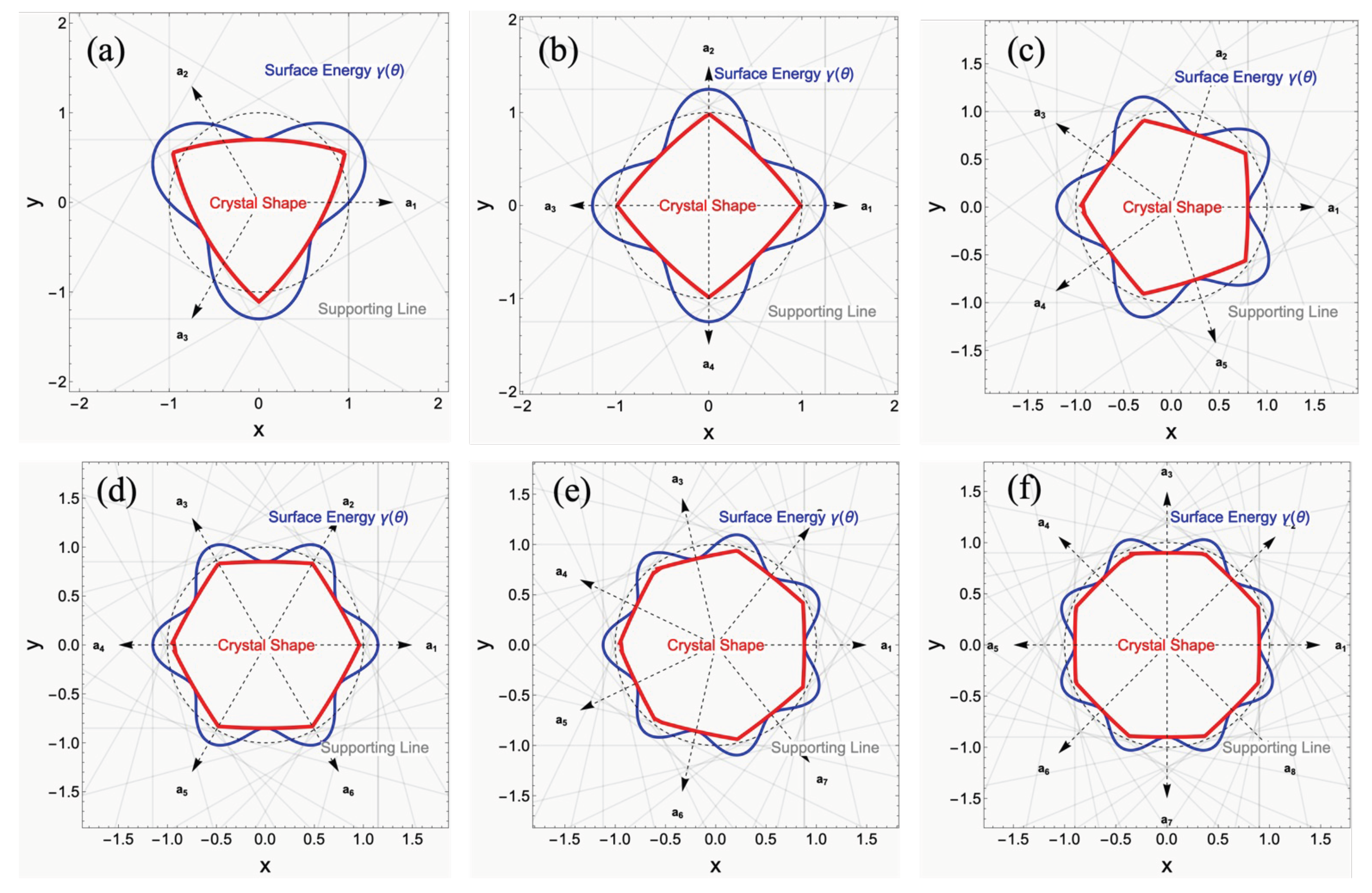
We plotted the Wulff construction for two-dimensional crystals with arbitrary N-fold symmetry as shown in Figure 1 through the following steps. First, the surface energy $\gamma \left(\theta \right)$, which represents the interfacial energy of the crystal in different directions, is defined as a function in polar coordinates as $\gamma \left(\theta \right)=1+ϵcos\left[n\right(\theta -\varphi \left)\right]$, where n is the symmetry order and $ϵ$ controls the anisotropy strength. The program uses PolarPlot to draw this function in polar coordinates, resulting in a closed blue curve. The distance from each point on the curve to the origin represents the surface energy in that direction. Second, the supporting lines are lines perpendicular to each direction whose distance from the origin is exactly equal to the surface energy in that direction, given by the equation $xcos\theta +ysin\theta =\gamma \left(\theta \right)$. The program selects a set of discrete directions (spaced by $\pi /\left(2n\right)$), computes a point (the foot of the perpendicular) and a direction vector for each line, and draws them as gray, semi-transparent lines. These lines collectively “support” the crystal shape. Finally, the crystal shape is the region of points satisfying all the supporting line inequalities ($xcos\theta +ysin\theta \le \gamma \left(\theta \right)$), i.e., the intersection of all the half-planes bounded by these lines. The program discretizes a large number of angles (300 in this work) to construct half-plane constraints, uses a region intersection algorithm to compute the polygonal boundary of the intersection, and connects the vertices into a closed red polygon. These three graphical elements are overlaid to visually demonstrate how the surface energy, via the constraints of the supporting lines, determines the equilibrium shape of the crystal. The complete computational procedure is summarized in Algorithm 1.

4.2. Pseudocode for Wulff Construction

Algorithm 1 Wulff construction for 2D crystals with N-fold symmetry.

Require: Symmetry order N, anisotropy $ϵ$, phase $\varphi$, number of discrete points M Ensure: Vertices of the Wulff shape polygon   1: Define surface energy function: $\gamma \left(\theta \right)=1+ϵcos\left(N\right(\theta -\varphi \left)\right)$   2: Initialize an empty list of half-plane constraints   3: for $i=0$ to $M-1$ do   4:     ${\theta }_i=2\pi i/M$   5:     $a_i=cos\left({\theta }_i\right)$   6:     $b_i=sin\left({\theta }_i\right)$   7:     $c_i=\gamma \left({\theta }_i\right)$   8:     Add constraint: $a_{i}x+b_{i}y\le c_i$ to the list   9: end for 10: Define region R as the intersection of all half-planes 11: Compute the boundary of R as a convex polygon 12: Extract vertices of the polygon 13: return vertices

4.3. Visualization Steps

To visualize the construction, we outline the key steps in Algorithm 2. It takes the vertices produced by Algorithm 1 as input and generates the plots of the surface energy profile, supporting lines, and the final Wulff shape.

Algorithm 2 Visualization of Wulff construction.

Require: Vertices from Algorithm 1, N, $ϵ$, $\varphi$ Ensure: Plot of $\gamma$ plot, supporting lines, and Wulff shape   1: Create polar plot of $\gamma \left(\theta \right)$ for $\theta \in [0,2\pi )$ (blue curve)   2: For a sparse set of angles (e.g., every $\pi /\left(2N\right)$), draw the line $xcos\theta +ysin\theta =\gamma \left(\theta \right)$ (gray, semi-transparent)   3: Plot the polygon defined by the vertices (red, closed)   4: Add symmetry direction arrows and labels   5: Combine all plots with appropriate labels and legends

5. Discussion

Viewing the Wulff construction through the lens of Legendre duality demystifies its structure and connects it to broader concepts.

5.1. Connection to Statistical Mechanics and Large Deviations

In statistical mechanics, the Wulff shape emerges as the deterministic equilibrium profile in the macroscopic limit of lattice spin systems like the Ising model below the critical temperature [4,24,25,26]. The surface tension $\tau \left(\mathbf{n}\right)$ plays the role of $\gamma \left(\mathbf{n}\right)$. The large deviation principle for the phase boundary states that the probability of observing a droplet with a shape close to $\mathcal{W}$ is exponentially favored. The rate function is precisely the surface energy functional, and its minimization yields the Wulff shape. The Legendre transform structure is inherent in this large deviation formalism, linking microscopic fluctuations to the macroscopic convex duality [27]. Early exact solutions for equilibrium shapes in two-dimensional lattice models, such as the work by Rottman and Wortis [28], provided crucial microscopic validation of the Wulff construction and laid the groundwork for the rigorous large deviation theory that followed.

5.2. The Cahn–Hoffman $\xi$ Vector and Gradient Flows

A related formulation uses the Cahn–Hoffman $\xi$ vector defined such that $\gamma \left(\mathbf{n}\right)=\xi \left(\mathbf{n}\right)·\mathbf{n}$. The $\xi$ plot (the radial plot of the vector $\xi \left(\mathbf{n}\right)$) is exactly the polar plot of the duality of $\gamma$ in a different gauge. The equilibrium shape is given by the inner envelope (convex hull) of the $\xi$ plot, which is another geometric realization of the same Legendre duality. This framework is particularly useful for studying dynamics, as gradient flows of the surface energy often involve the chemical potential $\mu ={\kappa }_{\gamma }$, where ${\kappa }_{\gamma }$ is the anisotropic curvature derived from $\gamma$ and its derivatives.

The Cahn–Hoffman $\xi$-vector not only encodes the surface stress but also directly relates to the growth kinetics in anisotropic systems. In kinetic growth models, the $\xi$ plot’s convex hull can be interpreted as the limiting shape under surface attachment-limited kinetics, bridging the equilibrium thermodynamics and non-equilibrium growth morphology [29,30,31]. This connection becomes particularly evident in the context of the kinetic Wulff construction, where the growth velocity $v\left(\mathbf{n}\right)$ often inherits the directional dependence of the surface stress via the mobility tensor. Thus, the $\xi$ vector serves as a unifying geometric object that links static equilibrium shapes, dynamic growth fronts, and even the response to external fields or substrate interactions [32,33,34]. Beyond kinetics, the interplay between anisotropic surface energy and elastic strain represents another major frontier for extending Wulff’s theory. Studies on epitaxially strained films have formulated generalized Wulff-type problems incorporating elastic energy [35], providing a foundation for the coupled solid membrane systems discussed in the outlook below.

5.3. Beyond Equilibrium: Kinetics and Geometry

While the classical theory addresses equilibrium, the Legendre duality perspective may offer insights into kinetic shapes. In growth models where the normal velocity $v\left(\mathbf{n}\right)$ is a function of the orientation, the asymptotic shape (for a constant driving force) is given by a construction similar to Wulff’s but with $\gamma \left(\mathbf{n}\right)$ replaced by $v\left(\mathbf{n}\right)$ [5]. This “kinetic Wulff shape” can also be understood via a Hopf–Lax formula, which is a time-dependent generalization of the Legendre transform used to solve Hamilton–Jacobi equations. Thus, the geometric duality provides a bridge between equilibrium thermodynamics and non-equilibrium growth kinetics. This bridge is exemplified in studies of post-synthesis thermal evolution, where faceted metal nanocrystals, initially synthesized in nonequilibrium shapes, undergo surface-diffusion-mediated reshaping towards the equilibrium Wulff shape—a process critical for the stability of their functional properties and amenable to simulation by stochastic atomistic models [36]. Extensions beyond the classical paradigm also include size-dependent Wulff shapes in alloy nanoparticles, where finite-size and compositional effects modify the equilibrium morphology [37]. At the molecular scale, the prediction of crystal morphology bridges with computational chemistry, where the mapping of molecular conformational landscapes to stable crystal structures [38] informs the effective anisotropy of surface energies, which then serve as input for macroscopic Wulff constructions.

6. Conclusions and Perspective

We have provided a detailed exposition that re-establishes the Legendre transform as the mathematical cornerstone of the Wulff construction. By meticulously deriving the equilibrium shape from the variational principle and then explicitly identifying the Wulff shape $\mathcal{W}$ as the zero-sublevel set of the convex conjugate ${\gamma }^{*}\left(\mathbf{x}\right)$, we have clarified the profound duality between the surface energy function $\gamma \left(\mathbf{n}\right)$ and the equilibrium crystal shape.

This work shifted the emphasis from the Wulff construction as a graphical algorithm for materials applications to its fundamental role as a canonical example of convex duality in physical systems. It unifies concepts from differential geometry, calculus of variations, the Legendre–Fenchel transform, and statistical mechanics (large deviations). Recognizing this foundation is not merely an academic exercise; it provides a more robust and general framework for understanding existing theories and for formulating new ones that venture beyond the classical equilibrium paradigm, such as in kinetic growth or the behavior of active materials.

While the classical Wulff construction addresses isolated crystals in a vacuum or homogeneous medium, many modern applications involve crystals embedded in soft environments, such as lipid membranes [39] or other 2D fluid sheets [16]. In these systems, the equilibrium shape of a solid domain is not only determined by its own edge energy (the 1D analog of surface energy) but also by elastic interactions mediated by the surrounding fluid membrane. Recent studies have explored how rigid planar inclusions (such as 2D colloidal plates) can adopt nontrivial shapes and arrangements due to long-range elastic deformations of the membrane [16,17]. These works reveal that the effective interactions between domains can lead to switchable positioning, shape transformations, and the self-assembly of complex patterns (e.g., flower-shaped crystals) on planar monolayers [18], curved vesicles [17], as well as entropy-driven 2D separated microdomains [40,41]. A promising application for precise intracellular drug delivery by designing an appropriate shape of organ-conformal, kirigami-structured bioelectronic patch [42] is an important interdisciplinary area of considerable interest.

The theoretical framework developed in the present work—centered on the variational principle and Legendre duality—provides a natural foundation for extending the Wulff construction to such coupled systems. By incorporating the elastic energy of the membrane into the total free energy functional, one can formulate a generalized Wulff problem that simultaneously minimizes the edge energy of the solid domain and the bending energy of the surrounding fluid membrane. The resulting equilibrium shapes are expected to deviate from the classical Wulff shape, exhibiting boundary- or curvature-driven faceting or buckling, as observed in recent experiments [17,18]. Moreover, the Legendre transform perspective offers a powerful tool for dualizing the coupled problem, potentially revealing new convexity relations between the solid shape and the membrane curvature field.

Thus, the present study not only clarifies the mathematical roots of the classical Wulff construction but also paves the way for future theoretical investigations of solid–membrane composite systems. By combining the geometric language of support functions with the elasticity theory of fluid membranes, one may develop predictive models for designing 2D functional materials, biosensors, and programmable vesicles with controlled solid inclusions.

References

1. Wulff, G. Xxv. zur frage der geschwindigkeit des wachsthums und der auflösung der krystallflächen. Z. Für Krist.-Cryst. Mater. 1901, 34, 449–530. [Google Scholar] [CrossRef] [Scilit]
2. Taylor, J.E. Crystalline variational problems. Bull. Am. Math. Soc. 1978, 84, 568–588. [Google Scholar] [CrossRef] [Scilit]
3. Khare, S.; Kodambaka, S.; Johnson, D.; Petrov, I.; Greene, J. Determining absolute orientation-dependent step energies: A general theory for the Wulff-construction and for anisotropic two-dimensional island shape fluctuations. Surf. Sci. 2003, 522, 75–83. [Google Scholar] [CrossRef] [Scilit]
4. Dobrushin, R.L.; Koteckỳ, R.; Shlosman, S. Wulff Construction: A Global Shape from Local Interaction; American Mathematical Society: Providence, RI, USA, 1992; Volume 104. [Google Scholar]
5. Osher, S.; Merriman, B. The Wulff shape as the asymptotic limit of a growing crystalline interface. Asian J. Math. 1997, 1, 560–571. [Google Scholar] [CrossRef] [Scilit]
6. Netzer, F.P.; Noguera, C. Oxide Thin Films and Nanostructures; Oxford University Press: Oxford, UK, 2021. [Google Scholar]
7. de Almeida, T.S. Convex geometric reasoning for crystalline energies. arXiv 2021, arXiv:2102.12683. [Google Scholar] [CrossRef] [Scilit]
8. McCann, R.J. Equilibrium shapes for planar crystals in an external field. Commun. Math. Phys. 1998, 195, 699–723. [Google Scholar] [CrossRef] [Scilit]
9. Brazitikos, S.; Giannopoulos, A.; Valettas, P.; Vritsiou, B.H. Geometry of Isotropic Convex Bodies; American Mathematical Society: Providence, RI, USA, 2014; Volume 196. [Google Scholar]
10. Wills, J. Wulff-shape, minimal energy, maximal density. Ferroelectrics 2001, 250, 157–161. [Google Scholar] [CrossRef] [Scilit]
11. Micheletti, A.; Patti, S.; Villa, E. Crystal growth simulations: A new mathematical model based on the Minkowski sum of sets. Ind. Days 2003-2004 2005, 2, 130–140. [Google Scholar]
12. Marks, L.; Peng, L. Nanoparticle shape, thermodynamics and kinetics. J. Physics Condens. Matter 2016, 28, 053001. [Google Scholar] [CrossRef] [Scilit]
13. Shi, A.C.; Wortis, M. Equilibrium shape of NaCl crystals: A first-principles calculation. Phys. Rev. B 1988, 37, 7793. [Google Scholar] [CrossRef] [Scilit]
14. Gao, Y.; Song, W.; Yang, J.; Ji, X.; Wang, N.; Huang, X.; Wang, T.; Hao, H. Crystal morphology prediction models and regulating methods. Crystals 2024, 14, 484. [Google Scholar] [CrossRef] [Scilit]
15. Wortis, M. Equilibrium crystal shapes and interfacial phase transitions. In Chemistry and Physics of Solid Surfaces VII; Springer: Berlin, Germany, 1988; pp. 367–405. [Google Scholar]
16. Xin, W.; Wu, H.; Grason, G.M.; Santore, M.M. Switchable positioning of plate-like inclusions in lipid membranes: Elastically mediated interactions of planar colloids in 2D fluids. Sci. Adv. 2021, 7, eabf1943. [Google Scholar] [CrossRef] [Scilit]
17. Wan, H.; Jeon, G.; Xin, W.; Grason, G.M.; Santore, M.M. Flower-shaped 2D crystals grown in curved fluid vesicle membranes. Nat. Commun. 2024, 15, 3442. [Google Scholar] [CrossRef] [Scilit]
18. Wu, H.; Tu, Z. Theoretical and numerical investigations on shapes of planar lipid monolayer domains. J. Chem. Phys. 2009, 130, 045103. [Google Scholar] [CrossRef] [Scilit]
19. Wu, H.; Ou-Yang, Z.C.; Podgornik, R. Continuum theory of electrostatic-elastic coupling interactions in colloidal crystals. Commun. Theor. Phys. 2025, 77, 055602. [Google Scholar] [CrossRef] [Scilit]
20. Wu, H.; Ou-Yang, Z.C.; Podgornik, R. Electrostatic-elastic coupling in colloidal crystals. Europhys. Lett. 2024, 148, 47001. [Google Scholar] [CrossRef] [Scilit]
21. Duan, W.; Mu, Y.; Mo, X.; Wang, Z.; Zhang, T.; Ho, Y.Y.L.; Lyu, D.; Zhang, D.; Zhao, R.; Tse, E.C.M.; et al. Chemical Auxiliary for Photocatalytic Active Colloids. J. Am. Chem. Soc. 2024, 146, 26505–26515. [Google Scholar] [CrossRef] [Scilit]
22. Ulivelli, J. First variation of functional Wulff shapes. Adv. Math. 2025, 480, 110529. [Google Scholar] [CrossRef] [Scilit]
23. Zia, R. Anisotropic surface tension and equilibrium crystal shapes. In Progress in Statistical Physics; Hu, C.K., Ed.; World Scinetific: Singapore, 1988; pp. 303–357. [Google Scholar]
24. Pisztora, A. Surface order large deviations for Ising, Potts and percolation models. Probab. Theory Relat. Fields 1996, 104, 427–466. [Google Scholar] [CrossRef]
25. Bodineau, T.; Ioffe, D.; Velenik, Y. Rigorous probabilistic analysis of equilibrium crystal shapes. J. Math. Phys. 2000, 41, 1033–1098. [Google Scholar] [CrossRef] [Scilit]
26. Cerf, R. The Wulff Crystal in Ising and Percolation Models: Ecole d’Eté de Probabilités de Saint-Flour XXXIV-2004; Springer: Berlin, Germany, 2006. [Google Scholar]
27. Ioffe, D. Large deviations for the 2D Ising model: A lower bound without cluster expansions. J. Stat. Phys. 1994, 74, 411–432. [Google Scholar] [CrossRef] [Scilit]
28. Rottman, C.; Wortis, M. Exact equilibrium crystal shapes at nonzero temperature in two dimensions. Phys. Rev. B 1981, 24, 6274. [Google Scholar] [CrossRef] [Scilit]
29. Cahn, J.; Hoffman, D. A vector thermodlnamics for anisotropic surfaces—II. Curved and faceted surfaces. Acta Metall. 1974, 22, 1205–1214. [Google Scholar] [CrossRef] [Scilit]
30. Hoffman, D.W.; Cahn, J.W. A vector thermodynamics for anisotropic surfaces: I. Fundamentals and application to plane surface junctions. Surf. Sci. 1972, 31, 368–388. [Google Scholar] [CrossRef] [Scilit]
31. Taylor, J.E. II—Mean curvature and weighted mean curvature. Acta Metall. Mater. 1992, 40, 1475–1485. [Google Scholar] [CrossRef] [Scilit]
32. Winterbottom, W.L. Equilibrium shape of a small particle in contact with a foreign substrate. Acta Metall. 1967, 15, 303–310. [Google Scholar] [CrossRef] [Scilit]
33. Zia, R.; Avron, J.; Taylor, J. The summertop construction: Crystals in a corner. J. Stat. Phys. 1988, 50, 727–736. [Google Scholar] [CrossRef] [Scilit]
34. Ringe, E.; Van Duyne, R.P.; Marks, L.D. Kinetic and thermodynamic modified Wulff constructions for twinned nanoparticles. J. Phys. Chem. C 2013, 117, 15859–15870. [Google Scholar] [CrossRef] [Scilit]
35. Bonacini, M. Epitaxially strained elastic films: The case of anisotropic surface energies. ESAIM: Control. Optim. Calc. Var. 2013, 19, 167–189. [Google Scholar] [CrossRef] [Scilit]
36. Lai, K.C.; Liu, D.J.; Huang, W.; Han, Y.; Evans, J.W. Thermal shape stability of fcc metal nanocrystals synthesized with faceted nonequilibrium shapes. J. Phys. Chem. C 2024, 128, 7026–7040. [Google Scholar] [CrossRef] [Scilit]
37. Ringe, E.; Van Duyne, R.P.; Marks, L. Wulff construction for alloy nanoparticles. Nano Lett. 2011, 11, 3399–3403. [Google Scholar] [CrossRef] [Scilit] [PubMed]
38. Thompson, H.P.; Day, G.M. Which conformations make stable crystal structures? Mapping crystalline molecular geometries to the conformational energy landscape. Chem. Sci. 2014, 5, 3173–3182. [Google Scholar] [CrossRef] [Scilit]
39. Wu, H.; Ou-Yang, Z.C. A Generalized Helfrich Free Energy Framework for Multicomponent Fluid Membranes. Membranes 2025, 15, 182. [Google Scholar] [CrossRef] [Scilit]
40. Wu, H.; Shiba, H.; Noguchi, H. Mechanical properties and microdomain separation of fluid membranes with anchored polymers. Soft Matter 2013, 9, 9907–9917. [Google Scholar] [CrossRef] [Scilit]
41. Wu, H.; Noguchi, H. Effects of anchored flexible polymers on mechanical properties of model biomembranes. AIP Conf. Proc. Am. Inst. Phys. 2013, 1518, 649–653. [Google Scholar]
42. Wang, Y.; Du, L.; Wu, H.; Li, H.; Liu, J.; Hu, Y.; Jiang, X.; Yin, D.; Hao, Y.; Xiao, A.; et al. An organ-conformal, kirigami-structured bioelectronic patch for precise intracellular delivery. Cell 2026. [Google Scholar] [CrossRef] [Scilit]
43. Akutsu, Y.; Akutsu, N. Relationship between the anisotropic interface tension, the scaled interface width and the equilibrium shape in two dimensions. J. Phys. A: Math. Gen. 1986, 19, 2813. [Google Scholar] [CrossRef] [Scilit]
Figure 1. The computed and plotted Wulff shapes for a 2D crystal with different N-fold symmetry: (a) three-fold symmetry, (b) four-fold symmetry, (c) five-fold symmetry, (d) six-fold symmetry, (e) seven-fold symmetry, and (f) eight-fold symmetry.
Crystals 16 00108 g001
Disclaimer/Publisher’s Note: The statements, opinions and data contained in all publications are solely those of the individual author(s) and contributor(s) and not of MDPI and/or the editor(s). MDPI and/or the editor(s) disclaim responsibility for any injury to people or property resulting from any ideas, methods, instructions or products referred to in the content.