Indexing 2D Powders and Lagrange–Gauss Reduction

Abstract

Two-dimensional (2D) powders constitute an important class of molecular thin films where a specific close-packed plane forms parallel to the substrate surface, while there is no preferred lateral ordering. Using results from classic lattice reduction theory, a systematic scheme is proposed in order to determine the 3D surface unit cell for 2D powders in reciprocal space. The approach is based on a sorted set of lengths $q_1,q_2,q_3,\dots$ of the in-plane components of the scattering vector, which is directly obtained from the scattering pattern. After a first match is established, a refinement procedure is presented that makes full use of the complete set of scattering vectors and, as such, corrects for small experimental errors and ensures a good overall match with the observed reflections. After identifying the in-plane components, the full 3D surface unit cell can be found in a straightforward way.

1. Introduction

A characteristic of functional thin films grown on smooth substrates, such as silicon wafers and glass slides, is that films crystallize with a specific crystallographic plane parallel to the substrate, while crystalline domains are randomly oriented laterally. Such 2D powders can be conveniently characterized with X-ray scattering techniques such as GISAXS or GIWAXS (grazing incidence small or wide-angle x-ray scattering, respectively), which make use of area detectors [1,2,3,4,5] or line detectors [4,6] and cover large parts of reciprocal space efficiently. While typically 10 to 50 reflections can be observed, this is by no means sufficient for an ab initio crystal structure determination. Nonetheless, usually the thin film lattice constants can be determined. In many cases the molecular lattice in the thin film is different from the bulk single crystal. Usually the structure of the molecule is known from single crystal diffraction, which is performed routinely after molecule synthesis. By determining the thin-film crystal lattice parameters, a rigid molecule approximation can be employed where the molecular structure is taken from single crystal data and then fit into the experimentally determined thin-film unit cell [7,8,9]. This way the molecular orientation on the substrate can be found, from which other properties, in particular the lateral and perpendicular charge mobilities, can be calculated and correlated with device performance.

Hence the determination of the thin-film molecular lattice, also known as indexing, is crucial for understanding the performance of molecular thin films [5,10,11,12,13,14]. Another fascinating aspect is polymorph control during thin-film processing [15,16,17,18,19,20,21]. In the following it will be discussed how to approach this problem for low-symmetry lattices that small molecules typically crystallize in and how insights from classical mathematics help to determine a compact surface unit cell.

2. Methods

The idea for this paper originated in a series of brain-storming sessions with Google Gemini 2.5 and Anthropic Claude Sonnet 4.5 about how to uniquely define a “best” unit cell for a 2D lattice. This brought classical work on number theory and contemporary work on cryptography to the author’s attention that is usually not referred to in modern crystallography. The properties of the 2D reduced unit cell have important consequences for solving the indexing problem for 2D powders.

3. Results and Discussion

In this section important concepts such as surface unit cells and scattering rods are introduced, and then the indexing problem will be discussed and illustrated with examples.

3.1. Bulk and Surface Unit Cell in Real and Reciprocal Space

When molecules crystallize on a smooth substrate, they often choose a molecular layer inside the bulk structure to form a dense-packed layer parallel to the substrate surface. This can be a low-index Miller plane such as (001), but sometimes such molecular layers are formed in different planes inside the crystallographic unit cell, such as (201) [22,23]. In the latter case the lattice vectors of the surface unit cell do not coincide with the bulk lattice vectors. The surface unit cell has some interesting properties, which help to solve the indexing problem.

With two lattice vectors lying in the surface plane, this means that the reciprocal surface unit cell, constructed in the usual way from the real-space surface unit cell of a multilayered thin film, will have a vector ${\stackrel{⃑}{c}}^{*}$ that is perpendicular to the reference surface. In contrast, the other reciprocal vectors will, in general, have components both parallel and perpendicular to the surface plane, in particular for triclinic lattices, where all angles between lattice vectors differ from 90°. Hence the indexing problem can be separated into finding the in-plane lattice parameters ${\stackrel{⃑}{a}}_{\parallel }^{*}$, ${\stackrel{⃑}{b}}_{\parallel }^{*}$ and the enclosed angle ${\gamma }_{\parallel }^{*}$ and then, as a second step, determining a solution for the perpendicular lattice parameters [5]. Here we will be mainly concerned with deriving the in-plane lattice parameters of the reciprocal surface unit cell.

3.2. Scattering Rods

For a 2D powder we established that the ${\stackrel{⃑}{c}}^{*}$ reciprocal lattice vector is perpendicular to the substrate surface. The diffraction spots form lines along ${\stackrel{⃑}{c}}^{*}$, the so-called scattering rods [23]. For stronger reflections one can also observe diffuse scattering streaks perpendicular to the surface, which originate from the truncation of the thin-film lattice at its surface [24,25]. Due to the nonlinear relationship between angular space and reciprocal space, the scattering rods often appear slightly curved in the detector image. However, with suitable software, the reflections along the rods can be extrapolated and so the in-plane $q$-vectors can be found, even if there are no reflections close to the horizon. This provides us with a sufficient number of in-plane scattering vectors, which will then be used for solving the in-plane lattice.

3.3. 2D Lattices and Lagrange–Gauss Reduction

A 2D lattice is given by two vectors ${\stackrel{⃑}{a}}_{\parallel }^{*}$ and ${\stackrel{⃑}{b}}_{\parallel }^{*}$ that are not colinear. Lattice points are given as

$$\stackrel{⃑}{q}\left(h,k\right)=h {\stackrel{⃑}{a}}_{\parallel }^{*}+k{\stackrel{⃑}{b}}_{\parallel }^{*}$$

(1)

yielding for the squared lengths

$$q^2\left(h,k\right)=h^2{a}_{\parallel }^{*2}+2 hk a_{\parallel }^{*} b_{\parallel }^{*} \mathrm{c}\mathrm{o}\mathrm{s}\left({\gamma }_{\parallel }^{*}\right)+k^2{b}_{\parallel }^{*2}$$

(2)

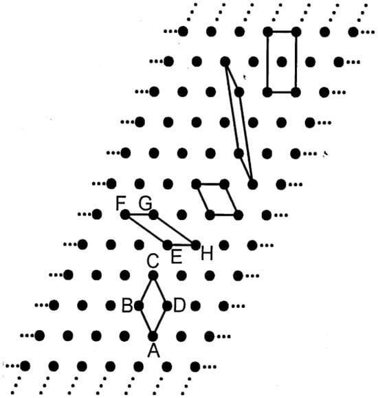
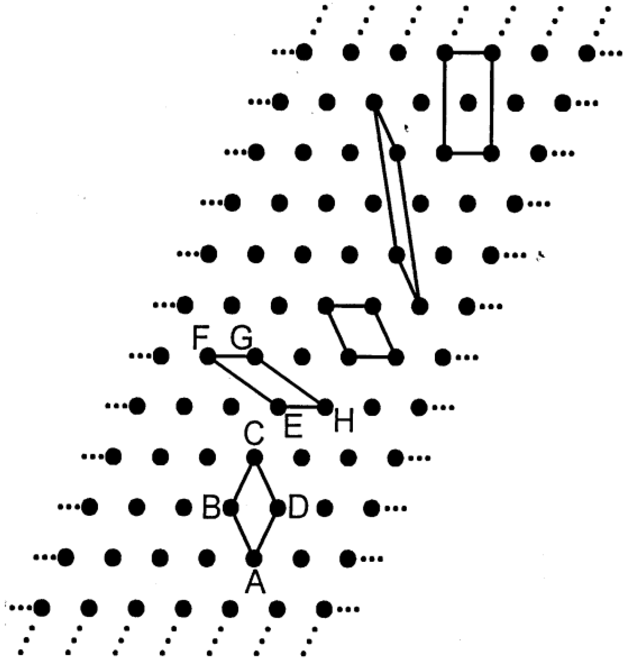
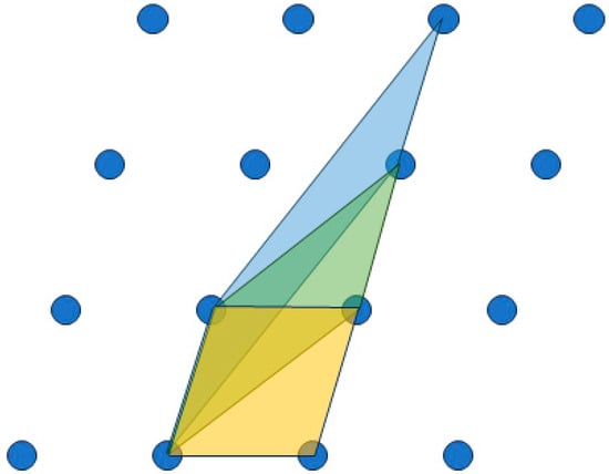
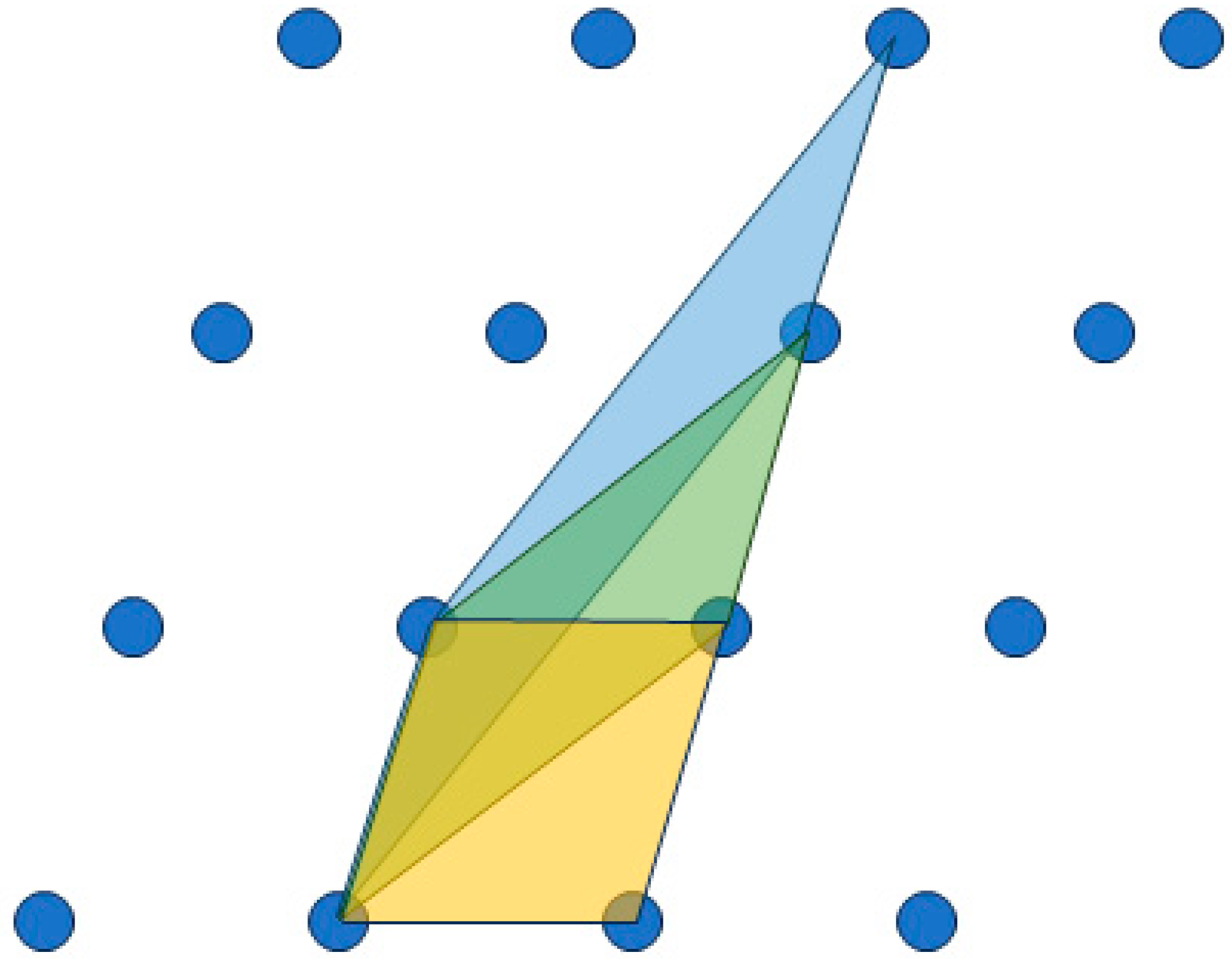
where $h,k\in \mathbb{Z}$ are integer numbers and ${\gamma }_{\parallel }^{*}$ is the enclosed angle between the parallel lattice vector components. We note that $q\left(\mathrm{1,0}\right)=a_{\parallel }^{*}$ and $q\left(\mathrm{0,1}\right)=b_{\parallel }^{*}$, i.e., $a_{\parallel }^{*}$ and $b_{\parallel }^{*}$ are contained within the set of lattice vectors, as is the origin. A well-known problem is that there is an infinite number of choices of ${\stackrel{⃑}{a}}_{\parallel }^{*}$ and ${\stackrel{⃑}{b}}_{\parallel }^{*}$ that can span the same lattice (see Figure 1). However, other than in higher dimensions, there is a well-defined way in two dimensions to uniquely extract a “best” choice of such vectors that was found in classic mathematics of the 18th century. Lagrange in 1773 and Gauss in 1801 independently encountered 2D lattices in the course of their studies on binary quadratic forms [26,27]. The Lagrange–Gauss algorithm can be easily described (see Figure 2): if there are two vectors generating the lattice, let us call the shorter one ${\stackrel{⃑}{a}}_{\parallel }^{*}$ and the other ${\stackrel{⃑}{b}}_{\parallel }^{*}$. Subtract ${\stackrel{⃑}{a}}_{\parallel }^{*}$ from ${\stackrel{⃑}{b}}_{\parallel }^{*}$ to obtain a new vector ${\stackrel{⃑}{b}}_{\parallel }^{*}$. If the new vector ${\stackrel{⃑}{b}}_{\parallel }^{*}$ is shorter, repeat. If ${\stackrel{⃑}{b}}_{\parallel }^{*}$ ends up being shorter than ${\stackrel{⃑}{a}}_{\parallel }^{*}$, exchange their roles. Eventually the length of the ${\stackrel{⃑}{b}}_{\parallel }^{*}$ vector cannot be reduced any further and the “best” base ${\stackrel{⃑}{a}}_{\parallel }^{*}$, ${\stackrel{⃑}{b}}_{\parallel }^{*}$ is found. Gauss proved that this will always be achieved in a finite number of steps; in fact, the algorithm is quite efficient.

This lattice reduction algorithm provides a finite scheme to obtain a unit cell with the two shortest possible lattice vectors ${\stackrel{⃑}{a}}_{\parallel }^{*}$ and ${\stackrel{⃑}{b}}_{\parallel }^{*}$ with lengths $a_{\parallel }^{*}\le b_{\parallel }^{*}$ and an enclosed angle ${\gamma }_{\parallel }^{*}$ close to 90°. In fact, from the algorithm, it follows directly [29,30] that

$$60°\le {\gamma }_{\parallel }^{*}\le 120°$$

(3)

where the equality is assumed for the hexagonal lattice with $a_{\parallel }^{*}=b_{\parallel }^{*}$.

Independent of specific unit cell choices, two 2D lattices are identical if there is a combination of rotations and translations that maps the lattice points onto each other. If we are only interested in the lengths of lattice vectors, as in our further analysis, two such lattices can be said to be equivalent when they can be brought to match if also a mirror reflection is involved. This is the case for any angle $0<\theta <30°$ and lattices that have the same $a_{\parallel }^{*}$ and $b_{\parallel }^{*}$ but ${\gamma }_{\parallel }^{*}=90°+\theta$ and ${\gamma }_{\parallel }^{*}=90°-\theta$. Thus the range of ${\gamma }_{\parallel }^{*}$ for equivalent lattices can be further reduced to

$$60°\le {\gamma }_{\parallel }^{*}\le 90°$$

(4)

Here we chose to have an acute angle between ${\stackrel{⃑}{a}}_{\parallel }^{*}$ and ${\stackrel{⃑}{b}}_{\parallel }^{*}$. This choice is consistent with the use of obtuse angles in real space and acute angles in reciprocal space in crystallography. Lagrange–Gauss reduction considerably reduces the available parameter space for the lattice parameters and also provides a unique parameter set, which has further important properties.

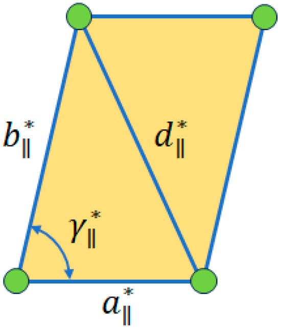
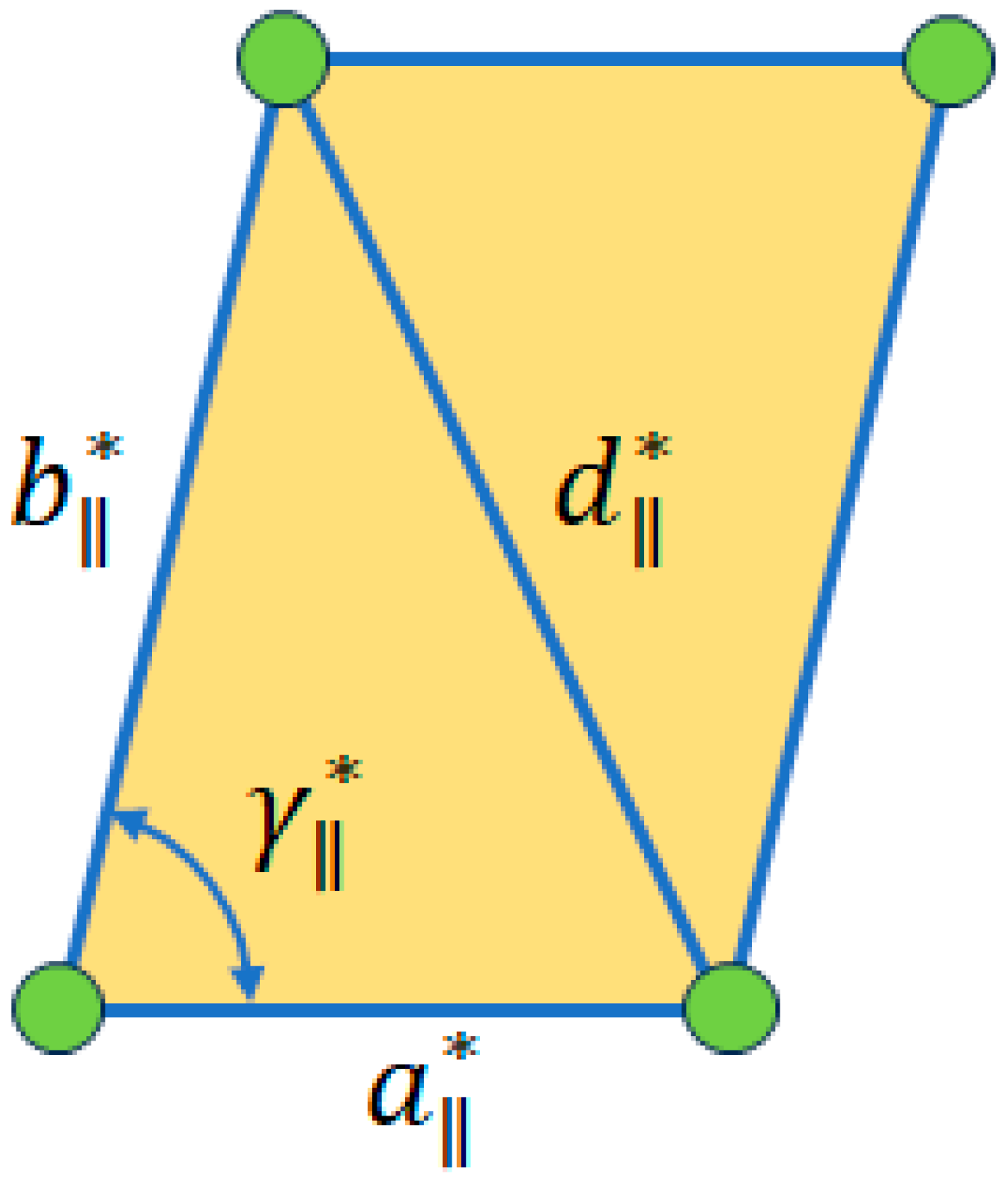
For a unit cell spanned by vectors ${\stackrel{⃑}{a}}_{\parallel }^{*}$ and ${\stackrel{⃑}{b}}_{\parallel }^{*}$, we obtain the lengths of the diagonals:

$$d_{\parallel }^{*}= q\left(-1, 1\right)=\left|{\stackrel{⃑}{b}}_{\parallel }^{*}-{\stackrel{⃑}{a}}_{\parallel }^{*}\right|=\sqrt{a_{\parallel }^{*2} + b_{\parallel }^{*2}-2a_{\parallel }^{*} b_{\parallel }^{*} cos\left({\gamma }_{\parallel }^{*}\right)}$$

(5a)

$${d\prime }_{\parallel }^{*}=q\left(1, 1\right)=\left|{\stackrel{⃑}{a}}_{\parallel }^{*}+{\stackrel{⃑}{b}}_{\parallel }^{*}\right|=\sqrt{a_{\parallel }^{*2}+b_{\parallel }^{*2}+2a_{\parallel }^{*} b_{\parallel }^{*} cos\left({\gamma }_{\parallel }^{*}\right)}$$

(5b)

With the choice of ${\gamma }_{\parallel }^{*}$ to be acute and, hence, $\cos \left({\gamma }_{\parallel }^{*}\right)>0$, $d_{\parallel }^{*}$ is the shorter diagonal (see Figure 3). Moreover, $d_{\parallel }^{*}$ is also the third shortest lattice vector with $b_{\parallel }^{*}\le d_{\parallel }^{*}\le {d\prime }_{\parallel }^{*}<2b_{\parallel }^{*}$, except for colinear multiples of ${\stackrel{⃑}{a}}_{\parallel }^{*}$, which will be ignored. All in all, we obtain an alternative way to uniquely describe the lattice by the set of vectors of shortest lengths $a_{\parallel }^{*}, b_{\parallel }^{*},d_{\parallel }^{*}$ that are not pairwise colinear. This is due to the fact that a triangle is uniquely given by two sides and the enclosed angle or, alternatively, by three sides (see Figure 3). The importance of the cell diagonal was realized in the classic works of Selling and Delaunay as well as Niggli in their efforts to determine a uniquely defined unit cell in three dimensions [31,32,33].

3.4. The Indexing Problem

The latter description of the reduced unit cell is well suited to tackle the indexing problem for the 2D lattice of the parallel components. From the analysis of a GIWAXS image, a series of $q$-values can be derived with

$$q_1<q_2<q_3<\cdots$$

(6)

If we can assume that we have observed a complete set of $q$-values and considering the properties of the “best” unit cell, we can identify the first $q$-values in this sorted set with $a_{\parallel }^{*}, b_{\parallel }^{*}$, and $d$ if we carefully include special cases:

Case 1: Hexagonal lattice

$${a_{\parallel }^{*}=b_{\parallel }^{*}=d_{\parallel }^{*}=q}_1: {\gamma }_{\parallel }^{*}=60°$$

(7)

Case 2: Rhombic lattice (including square)

$$a_{\parallel }^{*}=b_{\parallel }^{*}=q_1, d_{\parallel }^{*}=q_2: {\gamma }_{\parallel }^{*}=\mathrm{a}\mathrm{r}\mathrm{c}\mathrm{c}\mathrm{o}\mathrm{s}\left((2a_{\parallel }^{*2}-d_{\parallel }^{*2})/2a_{\parallel }^{*2}\right)$$

(8)

Case 3: Oblique lattice (including rectangular)

$$a_{\parallel }^{*}=q_1, b_{\parallel }^{*}=q_2,d_{\parallel }^{*}=q_3: {\gamma }_{\parallel }^{*}=\mathrm{a}\mathrm{r}\mathrm{c}\mathrm{c}\mathrm{o}\mathrm{s}\left((a_{\parallel }^{*2}+b_{\parallel }^{*2}-d_{\parallel }^{*2})/2a_{\parallel }^{*} b_{\parallel }^{*}\right)$$

(9)

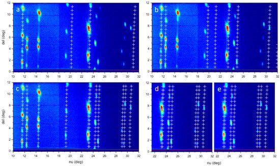
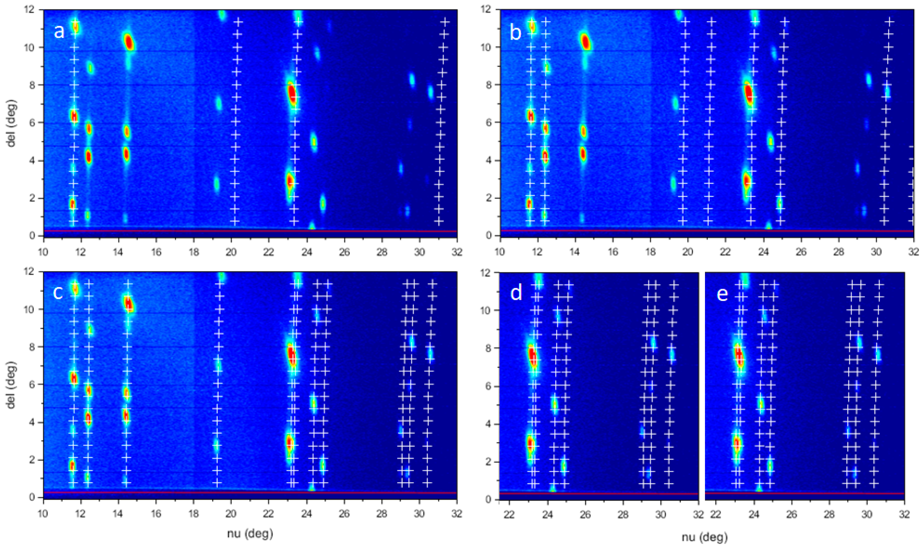
From the best match of these three cases, we can calculate $q\left(h,k\right)$ for a suitable range of $h$ and $k$ and then sort them by length and compare this sequence with the experimentally obtained sequence. This approach avoids guessing of indices $h,k$ but instead relies on sorting $q_i$ by length, which will also be of importance for the further refinement step. Figure 4 illustrates how the scattering rods determined by the three possible cases compare and it can be clearly seen that Case 3 is the correct choice in this example. Figure 4 was generated using the reciprocal space mode of program indexGIXS (Version 2T) [34]. The test data set was obtained from a thin film of the conjugated molecule TES-ADT (5,11-bis (triethyl silylethynyl) anthradithiophene) [35]. For details see the Supplementary Materials.

3.5. Further Refinement

After having established a good starting point, the lattice constants can be refined further. Since we only made use of the first three $q_i$ for the starting point at most, we have to take into account that small experimental errors remain, which can affect the match for the higher $q_i$, in particular for triclinic lattices. Hence it is desirable to include all observed $q_i$ in the refinement, in order to improve the overall match and make full use of the available information. The next task is to relate the calculated spots with the measured sequence. It is important for this step to identify possible overlapping spots or spots that are too weak to be observed. Below, in

Table 1. Sorted $q$-values and their Miller indices $h,k$ based on the initial starting point and matched up with $q$-values from the observed sequence.

$\mathit{h}$	$\mathit{k}$	${\mathit{q}}_{\mathit{i}}^{\mathit{c}\mathit{a}\mathit{l}\mathit{c}}$	${\mathit{q}}_{\mathit{i}}^{\mathit{e}\mathit{x}\mathit{p}}$
1	0	8.82	8.82 *
0	1	9.40	9.40 *
1	1	10.95	10.95 *
1	−1	14.57	14.5
2	1	17.52	17.45 **
2	0	17.64	17.45 **
1	2	18.40	18.33
0	2	18.80	18.75
2	2	21.9	21.8
2	−1	22.18	22.1
1	−2	22.89	22.9

* The initial assignment. ** Closely spaced calculated $q$ vectors get assigned the same experimentally determined $q$-value assuming spots were closely spaced and not resolved, as judged by the scattering pattern and calculated values. In a case where $q$-values should have been resolved but no spot was observed, the $q$-value is eliminated from the refinement.

, the matching of calculated and experimental data is illustrated based on the example shown in Figure 4.

Using this table we now have a system of equations that can be linearized:

$$q_{exp}^2\left(h,k\right)=h^2 X+k^2 Y+hk Z$$

(10)

with

$$X=a_{\parallel }^{*2} ,\hspace{1em}Y=b_{\parallel }^{*2},\hspace{1em}Z=2{ a}_{\parallel }^{*} b_{\parallel }^{*}\cos \left({\gamma }_{\parallel }^{*}\right)$$

(11)

by rewriting Equation (2). This system of equations is overdetermined, but a least-squares optimization can be performed. We construct the matrix M with columns $h^2, k^2$, and $hk$ for all $q_i$:

$$M=\left({ h}^2 \left| k^2 \right| hk\right).$$

(12)

The equation system can be written then as

$$M\left(\begin{array}{c}X\\ Y\\ Z\end{array}\right)=\left(q_{exp}^2\right).$$

(13)

The least-squares problem leads to the normal equations:

$$M^{T}M\left(\begin{array}{c}X\\ Y\\ Z\end{array}\right)=M^T\left(q_{exp}^2\right),$$

(14)

and its solution $X,Y,Z$ yields the refined reciprocal lattice constants:

$$a_{\parallel }^{*} =\sqrt{X}, b_{\parallel }^{*}=\sqrt{Y}, {\gamma }_{\parallel }^{*}=\mathrm{a}\mathrm{r}\mathrm{c}\mathrm{c}\mathrm{o}\mathrm{s}(Z/2{ a}_{\parallel }^{*} b_{\parallel }^{*})$$

(15)

For TES-ADT we found the following lattice parameters for the in-plane components of the reciprocal surface unit cell: $a_{\parallel }^{*}=$ 8.76 nm⁻¹, $b_{\parallel }^{*}=$ 9.39 nm⁻¹, and ${\gamma }_{\parallel }^{*}=$ 73.66°.

3.6. Reconstructing the 3D Surface Unit Cell

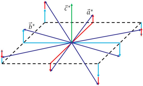
When the 2D lattice of the parallel lattice vector components has been found, it is straightforward to obtain the perpendicular components. If the data set covers the $\left(00l\right)$ scattering rod, $c^{*}$ can be determined directly from the $q_{\perp }$-value of the lowest diffraction spot along the scattering rod. Similarly $a_{\perp }^{*}$ and $b_{\perp }^{*}$ can be directly obtained from the $\left(10l\right)$ and $\left(01l\right)$ scattering rods, respectively, by determining the position of the diffraction spots with the lowest perpendicular components (see Figure 5). If $\left(00l\right)$ is not part of the data set, $c^{*}$ can be obtained by matching the spacing of the diffraction spots on the two special scattering rods. Then a similar refinement as outlined in Section 3.5 can be performed, now for the full 3D lattice associated with the reciprocal surface unit cell [5]. With this information the 3D lattice vectors of the reciprocal surface unit cell can be reconstructed

$${\stackrel{⃑}{a}}^{*}=\left(\begin{array}{c}{a}_{\parallel }^{*}\\ 0\\ a_{\perp }^{*}\end{array}\right),\hspace{1em}{\stackrel{⃑}{b}}^{*}=\left(\begin{array}{c}{b}_{\parallel }^{*} \mathrm{c}\mathrm{o}\mathrm{s}\left({\gamma }_{\parallel }^{*}\right)\\ b_{\parallel }^{*} \mathrm{s}\mathrm{i}\mathrm{n}\left({\gamma }_{\parallel }^{*}\right)\\ b_{\perp }^{*}\end{array}\right),\hspace{1em}{\stackrel{⃑}{c}}^{*}=\left(\begin{array}{c}0\\ 0\\ c^{*}\end{array}\right)$$

(16)

and then back-transformed to the more familiar real-space surface unit cell.

Finally the standard lattice parameters are obtained as the lengths of the lattice vectors and the angles between the lattice vectors [5]. As for the example shown in Figure 4, the thin-film surface unit cell for triclinic TES-ADT was found to have the lattice parameters $a=$ 0.70 nm, $b=$ 0.75 nm, $c=$ 1.76 nm, $\alpha =$ 96.6°, $\beta =$ 92.3°, and $\gamma =$ 106.0°, slightly distorted from the bulk unit cell parameters $a=$ 0.67 nm, $b=$ 0.73 nm,$c=$ 1.67 nm, $\alpha =$ 98.1°, $\beta =$ 94.5°, and $\gamma =$ 103.9°.

3.7. Forbidden Scattering Rods

For monoclinic lattices with the common space group p2₁/a, the whole $\left(10l\right)$ scattering rod is forbidden when (001) is the texture plane parallel to the surface. Note that this is a rather restrictive condition; it only occurs for glide planes and only for a specific orientation of the molecular planes so that the glide translation vector lies in the molecular plane. Nonetheless this situation is not uncommon; for instance, polymorphs of anthracene, pyrene, and perylene assume such thin-film structures [5].

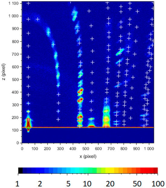
The whole $\left(10l\right)$ scattering rod being forbidden means that we have to assign $q_1$ as $b_{\parallel }^{*}$ and $q_2$ as $d_{\parallel }^{*}$. Next we have to consider all higher $q_i$ with $i\ge 3$, for which $q_i/2<d_{\parallel }^{*}$, and then tentatively assign ${ a}_{\parallel }^{*}$ to be $q_i/2$. We should find a promising match of experimental and calculated $q_i$ in a finite number of trials. This process is illustrated in

Table 2. Identification of lattice parameter ${ a}_{\parallel }^{*}$ for a monoclinic unit cell with a glide plane that renders the $\left(10l\right)$ rod forbidden. The headers indicate which $q_i$ was tested to be a candidate for $2{ a}_{\parallel }^{*}=q(2,0)$.

${\mathit{a}}_{\parallel }^{\mathit{*}}={\mathit{q}}_3/2$	${\mathit{a}}_{\parallel }^{\mathit{*}}={\mathit{q}}_4/2$	${\mathit{a}}_{\parallel }^{\mathit{*}}={\mathit{q}}_5/2$	${\mathit{a}}_{\parallel }^{\mathit{*}}={\mathit{q}}_6/2$	${\mathit{a}}_{\parallel }^{\mathit{*}}={\mathit{q}}_7/2$	${\mathit{q}}_{\mathit{e}\mathit{x}\mathit{p}}$
8.00	8.00	8.0	8.00	8.00	8.0
8.00	9.60	10.65	11.40	8.10	— *
8.89	11.64	13.3	13.30	9.07	13.30 **
13.30	13.30	13.34	14.53	13.30	13.30
14.91	16.00	16	16.00	15.07	16.00
14.91	17.51	19.19	18.76	15.03	19.2
16.00	19.20	19.26	20.50	16.00	19.2
16.00	19.74	21.30	22.80	16.20	21.30
17.79	19.78	22.73	23.45	18.15	(22.80) ***
20.44	21.77	22.78	24.00	20.40	(22.80) ***
20.44	23.27	12.00	24.86	20.57	— ****
22.21	24.00	26.23	25.59	22.36	26.2
22.21	24.62	26.29	26.60	29.36	26.2

* Forbidden by glide plane, ** assigned as $d$, *** very weak reflections, **** not observed—too weak.

for the case of C8-BTBT (2,7-dioctyl [1]benzothieno [3,2-b][1]benzothiophene), a conjugated molecule with excellent charge mobility [36]. Figure 6 shows a typical GIWAXS pattern for a thin film of C8-BTBT deposited on a silicon wafer, which could be indexed following this procedure. The streak-like shape on the diffraction spots is due to the small sample-detector distance compared to the width of the sample [37]. For details see the Supplementary Materials.

It is straightforward to generate the trial assignments for ${ a}_{\parallel }^{*}$ using Equation (2) and see also the Supplementary Materials. Correlation with the measured values takes some careful reasoning with regard to resolution and to identify unobserved reflections. Nonetheless, it becomes quickly clear that only choice of $q_5$ provides an overall good match with $q_{exp}$. Following the procedure outlined in Section 3.5 and Section 3.6 the thin-film lattice of C8-BTBT was found to be identical to the bulk structure [36] with lattice parameters $a=$ 0.593 nm, $b=$ 0.788 nm, $c=$ 2.918 nm, and $\beta =$ 92.4°.

We note that this procedure can also be applied to molecule lattices with space group p2₁/c and a (100) growth plane by transforming the lattice to yield space group p2₁/a [24]. Space group p2₁/a was highlighted here, because it fits in a natural way with the conventions of the surface unit cell. This scheme can also be employed in case there is reason to believe that one of the first three scattering rods is too weak to be observed.

Finally we note that space-group forbidden scattering rods can also occur in the orthorhombic system when the low-index molecular planes (100), (010), or (001) are formed parallel to the substrate surface. According to the current statistics of the Cambridge Structural Database, only 5.5% of known molecular structures have a higher symmetry, while triclinic (26.2%) and monoclinic structures (51.4%) are the most common [38].

3.8. Multiples of $a_{\parallel }^{*}$

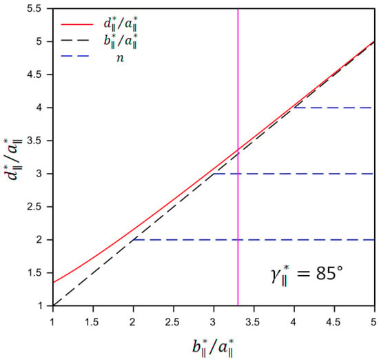
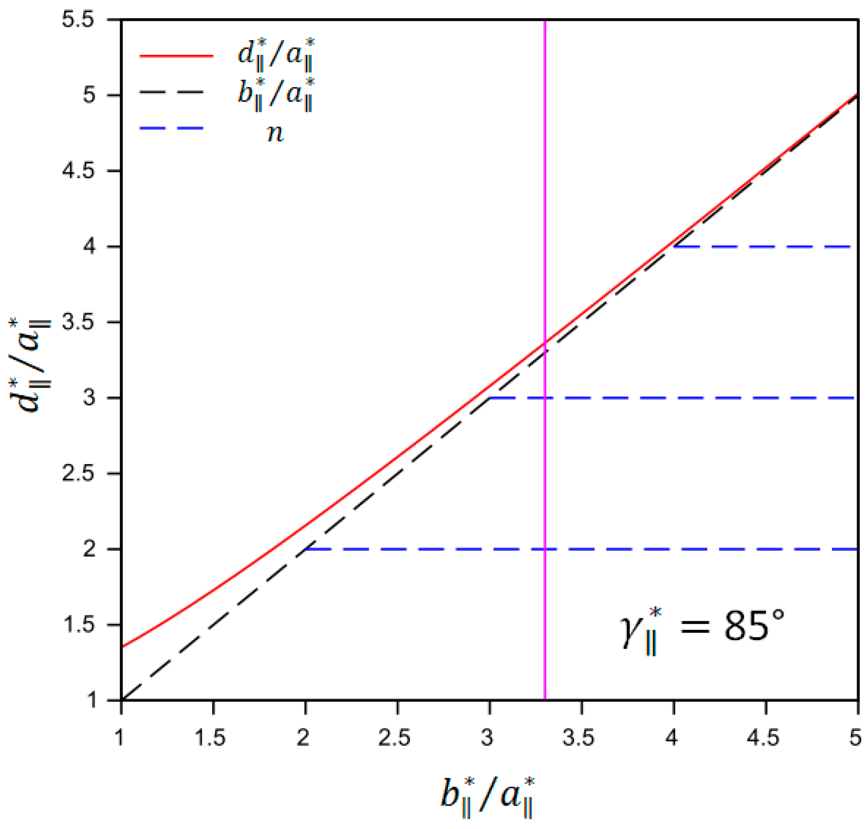
Multiples of ${ a}_{\parallel }^{*}$ can be a problem when ${ a}_{\parallel }^{*}$ is much smaller than $b_{\parallel }^{*}$, i.e., when 2${ a}_{\parallel }^{*}$ and so forth are smaller than $b_{\parallel }^{*}$ or $d_{\parallel }^{*}$. However, such $q$-values can be easily identified and skipped over when assigning $b_{\parallel }^{*}$ and $d_{\parallel }^{*}$. Another issue to consider here is that $b_{\parallel }^{*}$ and $d_{\parallel }^{*}$ will be very close and may not be resolved, i.e., $b_{\parallel }^{*}\approx d_{\parallel }^{*}$ (see Figure 7). Equation (9) can be rewritten in this case as

$$a_{\parallel }^{*}=q_1, b_{\parallel }^{*}=d_{\parallel }^{*}=q_2,: {\gamma }_{\parallel }^{*}=\mathrm{a}\mathrm{r}\mathrm{c}\mathrm{c}\mathrm{o}\mathrm{s}\left(a_{\parallel }^{*}/2 b_{\parallel }^{*}\right)$$

(17)

which can be considered as Case 4. Otherwise the analysis can proceed the same way as in Case 3.

In such a case it should also be checked whether $q_1$ is not ${ a}_{\parallel }^{*}$ but actually $2{ a}_{\parallel }^{*}$, i.e., if the lattice is monoclinic with a forbidden scattering rod. If a match is still not successful, it should also be checked whether $b_{\parallel }^{*}$ accidentally coincides with a multiple of ${ a}_{\parallel }^{*}$ by constructing a similar table as Table 2.

3.9. Other Complications

Finally there can be additional reflections from either the substrate, another film polymorph, and some other impurity in the film. First thing to look for is whether there is a difference in the radial and tangential spot widths or the overall spot shape in order to identify such interlopers and remove them from consideration. Other than that, there would be multiple trials needed, with various combinations of spots taken out of consideration. In such a situation recent computational methods may be a better option [39,40,41,42]. This case is the worse case scenario for any kind of indexing approach but, fortunately, the likelihood that such a $q$-value would be among the first three $q$-values of the film is finite.

4. Conclusions

A systematic approach to indexing 2D powders is presented that makes use of results based on classic mathematical work by Lagrange and Gauss. The reduced reciprocal unit cell of a thin film has important properties; in particular, it establishes that the shortest in-plane $q$-vectors can be identified with $a_{\parallel }^{*}=q$(1, 0), $b_{\parallel }^{*}=q\left(0, 1\right)$, and $d_{\parallel }^{*}=q(1,-1)$. The method is particularly useful for primitive lattices of triclinic and monoclinic symmetry, which are formed by the vast majority of small molecules. Crystallographers have tackled such problems for 3D powder diffraction and found similar lattice reduction schemes in 3D, resulting in the modern convention for assigning bulk unit cells [43]. The case of 2D powders lies somewhere in between pure 2D and 3D systems, with the six lattice constants of highly textured molecular thin films separating into 3 + 3 parameters for the surface unit cell in reciprocal space. Making use of complete scattering rods to identify the in-plane $q_i$ should help to overcome the problem of missing reflections. For space-group forbidden scattering rods, a way to recover the missing $q$-value has been discussed.

The approach has been successfully applied to indexing triclinic and monoclinic lattices in organic semiconductors. While the focus here was on low-symmetry lattices, we note that the approach does not preclude application to lattices with higher symmetry. However, there are more extended glide-plane symmetries, in particular for the orthorhombic system, which can lead to more missing scattering rods. Such lattices are much less common for small molecules, though, and hence the presented approach should cover a large variety of molecular thin films. Although not exhaustively complete, the outlined approach provides a good starting point to find an indexation for the reciprocal surface unit cell from which the 3D surface unit cell in real space can then be obtained.

References

- Sirringhaus, H.; Brown, P.J.; Friend, R.H.; Nielsen, M.M.; Bechgaard, K.; Langeveld-Voss, B.M.W.; Spiering, A.J.H.; Janssen, R.A.J.; Meijer, E.W.; Herwig, P.; et al. Two-dimensional charge transport in self-organized, high-mobility conjugated polymers. Nature 1999, 401, 685–688. [Google Scholar] [CrossRef] [Scilit]
- Breiby, D.W.; Bunk, O.; Andreasen, J.W.; Lemke, H.T.; Nielsen, M.M. Simulating X-ray diffraction of textured films. J. Appl. Crystallogr. 2008, 41, 262–271. [Google Scholar] [CrossRef] [Scilit]
- Steele, J.A.; Solano, E.; Hardy, D.; Dayton, D.; Ladd, D.; White, K.; Chen, P.; Hou, J.; Huang, H.; Saha, R.A.; et al. How to GIWAXS: Grazing Incidence Wide Angle X-Ray Scattering Applied to Metal Halide Perovskite Thin Films. Adv. Energy Mater. 2023, 13, 2300760. [Google Scholar] [CrossRef] [Scilit]
- Werzer, O.; Kowarik, S.; Gasser, F.; Jiang, Z.; Strzalka, J.; Nicklin, C.; Resel, R. X-ray diffraction under grazing incidence conditions. Nat. Rev. Methods Primers 2024, 4, 15. [Google Scholar] [CrossRef] [Scilit]
- Smilgies, D.-M. Probing Functional Thin Films with Grazing Incidence X-Ray Scattering: The Power of Indexing. Crystals 2025, 15, 63. [Google Scholar] [CrossRef] [Scilit]
- Smilgies, D.-M.; Blasini, D.R.; Hotta, S.; Yanagi, H. Reciprocal space mapping and single-crystal scattering rods. J. Synchrotron Radiat. 2005, 12, 807–811. [Google Scholar] [CrossRef] [Scilit] [PubMed]
- Yoshida, H.; Inaba, K.; Sato, N. X-ray diffraction reciprocal space mapping study of the thin film phase of pentacene. Appl. Phys. Lett. 2007, 90, 181930. [Google Scholar] [CrossRef] [Scilit]
- Schiefer, S.; Huth, M.; Dobrinevski, A.; Nickel, B. Determination of the crystal structure of substrate-induced pentacene polymorphs in fiber structured thin films. J. Am. Chem. Soc. 2007, 129, 10316–10317. [Google Scholar] [CrossRef] [Scilit]
- Mannsfeld, S.C.B.; Tang, M.L.; Bao, Z. Thin film structure of triisopropylsilylethynyl-functionalized pentacene and tetraceno[2,3-b]thiophene from grazing incidence X-ray diffraction. Adv. Mater. 2011, 23, 127–131. [Google Scholar] [CrossRef] [Scilit] [PubMed]
- Li, R.; Ward, J.W.; Smilgies, D.-M.; Payne, M.M.; Anthony, J.E.; Jurchescu, O.D.; Amassian, A. Direct structural mapping of organic field-effect transistors reveals bottlenecks to carrier transport. Adv. Mater. 2012, 24, 5553–5558. [Google Scholar] [CrossRef] [Scilit]
- Lamport, Z.A.; Li, R.; Wang, C.; Mitchell, W.; Sparrowe, D.; Smilgies, D.-M.; Day, C.; Coropceanu, V.; Jurchescu, O.D. Organic thin films with charge-carrier mobility exceeding that of single crystals. J. Mater. Chem. C 2017, 5, 10313–10319. [Google Scholar] [CrossRef] [Scilit]
- Mas-Torrent, M.; Rovira, C. Role of Molecular Order and Solid-State Structure in Organic Field-Effect Transistors. Chem. Rev. 2011, 111, 4833–4856. [Google Scholar] [CrossRef] [Scilit]
- Hiszpanski, A.M.; Loo, Y.-L. Directing the film structure of organic semiconductors via post-deposition processing for transistor and solar cell applications. Energy Environ. Sci. 2014, 7, 592–608. [Google Scholar] [CrossRef] [Scilit]
- Jones, A.O.F.; Chattopadhyay, B.; Geerts, Y.H.; Resel, R. Substrate-Induced and Thin-Film Phases: Polymorphism of Organic Materials on Surfaces. Adv. Funct. Mater. 2016, 26, 2233–2255. [Google Scholar] [CrossRef] [Scilit]
- Giri, G.; Verploegen, E.; Mannsfeld, S.C.B.; Atahan-Evrenk, S.; Kim, D.H.; Lee, S.Y.; Becerril, H.A.; Aspuru-Guzik, A.; Toney, M.F.; Bao, Z. Tuning charge transport in solution-sheared organic semiconductors using lattice strain. Nature 2011, 480, 504–508. [Google Scholar] [CrossRef] [Scilit]
- Diao, Y.; Shaw, L.; Bao, Z.; Mannsfeld, S.C.B. Morphology control strategies for solution-processed organic semiconductor thin films. Energy Environ. Sci. 2014, 7, 2145–2159. [Google Scholar] [CrossRef] [Scilit]
- Wan, J.; Li, L.; Ulbrandt, J.G.; Smilgies, D.-M.; Hollin, J.; Whalley, A.C.; Headrick, R.L. Transient phases during fast crystallization of organic thin films from solution. APL Mater. 2016, 4, 016103. [Google Scholar] [CrossRef] [Scilit]
- Richter, L.J.; DeLongchamp, D.M.; Amassian, A. Morphology Development in Solution-Processed Functional Organic Blend Films: An In Situ Viewpoint. Chem. Rev. 2017, 117, 6332–6366. [Google Scholar] [CrossRef] [Scilit] [PubMed]
- Chen, M.; Peng, B.; Huang, S.; Chan, P.K.L. Understanding the Meniscus-Guided Coating Parameters in Organic Field-Effect-Transistor Fabrications. Adv. Funct. Mater. 2020, 30, 1905963. [Google Scholar] [CrossRef] [Scilit]
- Lu, Z.; Wang, C.; Deng, W.; Achille, M.T.; Jie, J.; Zhang, X. Meniscus-guided coating of organic crystalline thin films for high-performance organic field-effect transistors. J. Mater. Chem. C 2020, 8, 9133–9146. [Google Scholar] [CrossRef] [Scilit]
- Ren, C.; Cao, L.; Wu, T. Meniscus-Guided Deposition of Organic Semiconductor Thin Films: Materials, Mechanism, and Application in Organic Field-Effect Transistors. Small 2023, 19, 2300151. [Google Scholar] [CrossRef] [Scilit]
- Krause, B.; Dürr, A.C.; Ritley, K.; Schreiber, F.; Dosch, H.; Smilgies, D. Structure and growth morphology of an archetypal system for organic epitaxy: PTCDA on Ag (111). Phys. Rev. B 2002, 66, 235404. [Google Scholar] [CrossRef] [Scilit]
- Smilgies, D.-M.; Boudet, N.; Struth, B.; Yamada, Y.; Yanagi, H. Highly oriented POPOP films grown on the KCl (001) surface. J. Cryst. Growth 2000, 220, 88–95. [Google Scholar] [CrossRef] [Scilit]
- Feidenhans’l, R. Surface structure determination by X-ray diffraction. Surf. Sci. Rep. 1989, 10, 105–188. [Google Scholar] [CrossRef] [Scilit]
- Robinson, I.K.; Tweet, D.J. Surface X-ray diffraction. Rep. Prog. Phys. 1992, 55, 599–651. [Google Scholar] [CrossRef] [Scilit]
- Lagrange, J.-L. Recherches d’arithmétique. In Nouveaux Mémoires de l’Académie Royale des Sciences et Belles-Lettres de Berlin; Chrétien Fréderic Voss: Berlin, Germany, 1773; pp. 265–312. [Google Scholar]
- Gauss, C.F. Disquisitiones Arithmeticæ; Gerhard Fleischer: Leipzig, Germany, 1801. [Google Scholar]
- Mighell, A.D.; Karen, V.L.; Munro, R. Determination of Reduced Cells in Crystallography. Available online: https://nvlpubs.nist.gov/nistpubs/sp958-lide/188-190.pdf (accessed on 24 October 2025).
- Vallée, B. Gauss’ Algorithm Revisited. J. Algorithms 1991, 12, 556–572. [Google Scholar] [CrossRef] [Scilit]
- Hoffstein, J.; Pipher, J.; Silverman, J.H. An Introduction to Mathematical Cryptography; Springer: New York, NY, USA, 2008. [Google Scholar]
- Selling, E. Ueber die binären und ternären quadratischen Formen. J. Reine Angew. Math. (Crelle’s J.) 1874, 1874, 143–229. [Google Scholar]
- Delaunay, B. Neue Darstellung der geometrischen Kristallographie. Z. Kristallogr. 1933, 84, 109–149. [Google Scholar] [CrossRef] [Scilit]
- Niggli, P. Kristallographische und strukturtheoretische Grundbegriffe. In Handbuch der Experimentalphysik; Akademische Verlagsgesellschaft: Leipzig, Germany, 1928. [Google Scholar]
- Smilgies, D.-M.; Li, R. indexGIXS—Software for visualizing and interactive indexing of grazing-incidence scattering data. ChemRxiv 2022. [Google Scholar] [CrossRef] [Scilit]
- Lee, S.S.; Tang, S.B.; Smilgies, D.-M.; Woll, A.R.; Loth, M.A.; Mativetsky, J.M.; Anthony, J.E.; Loo, Y.-L. Guiding Crystallization Around Bends and Sharp Corners. Adv. Mater. 2012, 24, 2692–2698. [Google Scholar] [CrossRef] [Scilit]
- Izawa, T.; Miyazaki, E.; Takimiya, K. Molecular Ordering of High-Performance Soluble Molecular Semiconductors and Re-evaluation of Their Field-Effect Transistor Characteristics. Adv. Mater. 2008, 20, 3388–3392. [Google Scholar] [CrossRef] [Scilit]
- Smilgies, D.-M. Scherrer Grain-Size Analysis Adapted to Grazing-Incidence Scattering with Area Detectors. J. Appl. Cryst. 2009, 42, 1030–1034. [Google Scholar] [CrossRef] [Scilit]
- Cambridge Structural Database (CSD). CSD Crystal System Statistics 2025. Available online: https://www.ccdc.cam.ac.uk/media/CSD-Crystal-System-Statistics-2025.pdf (accessed on 24 December 2025).
- Simbrunner, J.; Simbrunner, C.; Schrode, B.; Röthel, C.; Bedoya-Martinez, N.; Salzmann, I.; Resel, R. Indexing of Grazing-Incidence X-Ray Diffraction Patterns: The Case of Fibre-Textured Thin Films. Acta Crystallogr. A Found. Adv. 2018, 74, 373–387. [Google Scholar] [CrossRef] [Scilit] [PubMed]
- Simbrunner, J.; Salzmann, I.; Resel, R. Indexing of Grazing-Incidence X-Ray Diffraction Patterns. Crystallogr. Rev. 2023, 29, 19–37. [Google Scholar] [CrossRef] [Scilit]
- Kainz, M.P.; Legenstein, L.; Holzer, V.; Hofer, S.; Kaltenegger, M.; Resel, R.; Simbrunner, J. GIDInd: An Automated Indexing Software for Grazing-Incidence X-Ray Diffraction Data. J. Appl. Crystallogr. 2021, 54, 1256–1267. [Google Scholar] [CrossRef] [Scilit]
- Savikhin, V.; Steinrück, H.G.; Liang, R.Z.; Collins, B.A.; Oosterhout, S.D.; Beaujuge, P.M.; Toney, M.F. GIWAXS-SIIRkit: Scattering Intensity, Indexing and Refraction Calculation Toolkit for Grazing-Incidence Wide-Angle X-Ray Scattering of Organic Materials. J. Appl. Crystallogr. 2020, 53, 1108–1129. [Google Scholar] [CrossRef] [Scilit]
- Mighell, A.D. Lattice Symmetry and Identification—The Fundamental Role of Reduced Cells in Materials Characterization. J. Res. Natl. Inst. Stand. Technol. 2001, 106, 983–995. [Google Scholar] [CrossRef] [Scilit] [PubMed]
Disclaimer/Publisher’s Note: The statements, opinions and data contained in all publications are solely those of the individual author(s) and contributor(s) and not of MDPI and/or the editor(s). MDPI and/or the editor(s) disclaim responsibility for any injury to people or property resulting from any ideas, methods, instructions or products referred to in the content. |
© 2026 by the author. Licensee MDPI, Basel, Switzerland. This article is an open access article distributed under the terms and conditions of the Creative Commons Attribution (CC BY) license.