Measuring Optical Scattering in Relation to Coatings on Crystalline X-Ray Scintillator Screens

Abstract

Scattered light makes up a significant amount of recorded intensities during tomographic imaging, thereby leading to severe misinterpretation and artifacts in the reconstructed volume images. Correcting artificial intensities that stem from scattered light, therefore, is of primary interest and demands quantitative measurements. While numerous methods have been developed to reduce X-ray scattering artifacts, fewer methods deal with optical scattering. In this study, a measurement method for determining optical scattering in scintillators is presented with the aim of further developing correction algorithms. A theoretical model based on internal multiple reflections was developed for this purpose. This model assumes an additive exponential kernel with a certain scattering length to the system’s point spread function. This assumption was confirmed, and the scatter length was estimated from three new different kinds of experiments (hgap, rect, and LSF) on the BM18 beamline of the European synchrotron. The experiments further revealed significant differences in scattering proportion and length when different coatings are applied to the front and back faces of crystalline LuAG scintillators. Anti-reflective coatings on the backside show an effect of reducing the scattering magnitude while reflective coatings on the front side increase the proportion of the unscattered signal and, thus, show proportionally less scattering than black coating or no front coating. In particular, roughened black coating is found to worsen optical scattering. In summary, our results indicate that a combination of reflective (front) and anti-reflective (back) coatings yields the least optical scattering and, hence, the best image quality.

1. Introduction

X-ray Computed Tomography (CT) attempts to reconstruct an object’s optical density by back-projecting attenuated rays that are recorded by detector pixels. While the microscopic mechanisms of attenuation can be either photoelectric absorption or scattering (Rayleigh or Compton), it is generally assumed that neither object-scattered photons nor secondary (fluorescent) photons reach the detector screen to a point where they would change the ray sums, which, therefore, obey an exponential attenuation law.

A similar assumption is made when modeling the detector screen, e.g., for image corrections. In the common case of energy integrating scintillators, the latter convert X-rays into bursts of optical photons. The optical diffusion of these photons, e.g., Mie scattering inside powder screens, is known to cause image blur in the range of a few pixels [1]. Li developed a composite scintillator to reduce light scattering in perovskite scintillators, enhancing spatial resolution and imaging performance [2]. Meanwhile, optical scattering in the range of several dozens, if not hundred pixels, is rarely mentioned.

Both object scattering and optical scattering inside the converter screen may occur simultaneously and constitute primary sources of error for the numerical reconstruction (hence, CT artifacts) of the object’s volumetric density. In both cases, further intensity is recorded by the detector pixels in addition to the correctly attenuated ray sums. Partridge et al. identified multiple reflections between the scintillation screen and mirrors as the main source of scattering and suggested using a louvre grid on the screen to reduce scattered light, significantly enhancing image quality [3]. Siewerdsen and Jaffray examined X-ray scatter in Cone Beam Computed Tomography systems with flat-panel imagers, quantifying parasitic scatter via scatter-to-primary energy fluence ratio (SPR). High SPR values (>100%) for large objects and wide cone angles caused artifacts like cup and streak distortions and impaired the reconstruction accuracy [4]. Engel et al. found that parasitic scatter intensities in CT scale with illuminated volume, with dual-source CT showing doubled scatter-induced artifacts, such as streaks and cupping, reducing Contrast-to-Noise Ratio [5]. Numerous methods have been developed to correct image artifacts caused by X-ray scattering. Some methods are based on modified measurement setups. Siewerdsen et al. recommended antiscatter grids to reduce artifacts like cupping and improve image uniformity under high scatter conditions [6], while Endo et al. proposed focused collimators and conventional grids, with collimators significantly reducing scatter and improving image noise [7]. While others have used algorithmic methods based on simulations or convolutions, Seibert and Boone used deconvolution with a point spread function (PSF) to remove X-ray scatter via Fourier domain filtering [8], and Maltz et al. employed frequency modulation with a modulator grid and non-linear Fourier filtering to attenuate scatter in cone-beam CT [9]. Other methods first perform measurements on a phantom, followed by artifact removal using this data [10].

In most cases, the artificial intensities constitute a ‘scatter image’, which is often depicted as a low pass filtered reflection of the correct attenuation image. Meanwhile, in the case of optical detector scattering, this filter kernel can be a reasonably assumed invariant to the position and orientation of the object (hence, it would not change during a scan), coherent as well as incoherent scattering by the object yield artificial values that need to be computed for every new object pose and that strongly depend on the object–detector distance as well as the solid angle captured by each detector pixel.

At synchrotron beamlines, CT imaging generally sets a long distance between the object and detector to allow for propagation-based phase contrasts to emerge. While laboratory micro-CT scanners often place the object at 50 cm or closer to a large area detector (typ. 40 cm side length), synchrotron experiments feature a small detector area (5 cm$\times 1.6$ cm or less) and the parallel beam allows for setting it several meters downstream of the object without a noticeable loss in flux. Consequently, incoherent Compton scattering is generally neglected in the error-discussion of synchrotron micro-CT scans while it remains a major issue in medical and industrial CT scanners even if those employ similar photon energies as the synchrotrons.

Note that the opposite is true for coherent Rayleigh scattering, which may alter the pixel intensities of synchrotron detectors, which capture a very small solid angle compared to their laboratory counterparts. Another difference between laboratory and synchrotron detectors is that the latter mostly employ transparent single crystals as converter screens while the former use the consolidated powder of micro structured translucent polycrystalline screens. In transparent crystals the phenomenon of optical scattering mainly occurs on the back and front surfaces of the screen. Hence, coating the latter can change the internal reflectivity and alter the characteristics of optical scattering inside the scintillator.

To date, only a few methods have been developed for measuring and potentially correcting optical scattering in scintillators. In this context, we aim to present a measurement method for determining optical scattering that can serve as a reference for the development of further improved algorithms [3,11]. We recently managed to improve the light collection efficiency of such a lens-coupled indirect detector (LCID), which used 2 mm thick LuAG with different front and back coatings. Observations showed, however, that a significant part of the recorded intensities from these screens stems from optically scattered light and, thus, constitutes an artificial signal.

2. Materials and Methods

2.1. Experimental Setup

The present study focuses on X-ray imaging by sychrotron light. In contrast to laboratory X-ray imaging, synchrotron light emerges from high-energy electrons (6 GeV) that emit hard X-ray beams of extreme brightness when interacting with magnetic dipoles in a particle storage ring [12]. Compared to laboratory cone-beam, synchrotron light is defined by quasi-parallel beam geometry.

BM18 was commissioned as a new phase-contrast microtomography instrument at the European Synchrotron ESRF [13]. The $1.56\mathrm{T}$ three-pole wiggler (3PW) source produces a continuous and coherent spectrum of up to $350\mathrm{keV}$. Multiple filters can be used to adjust the average energy of the polychromatic beam from $25\mathrm{keV}$ to $350\mathrm{keV}$ without affecting spatial coherence [14]. The present experiment uses $5\mathrm{mm}$ sapphire and $170\mathrm{mm}$ glassy carbon filters for defining an average photon energy of $106.4\mathrm{keV}$. These filters represent a standard configuration of BM18.

The exit window to the experimental hutch is located at $172\mathrm{m}$ downstream of the 3PW source. On the backside of the exit window, a quinary pair of horizontal and vertical slits (20 mm thick tungsten blades) restricts the footprint of the beam and, hence, the field of view (FoV) to a rectangular window of variable size. Typically, the window is set so that only the FoV of the active detector is illuminated. The experimental hutch houses, behind the sample stage, a large slide carrying multiple detectors. The latter can be placed at an arbitrary distance ranging from $5\mathrm{m}$ to $39\mathrm{m}$ with respect to the exit window and the slits. The measurement setup is shown schematically in Figure 1.

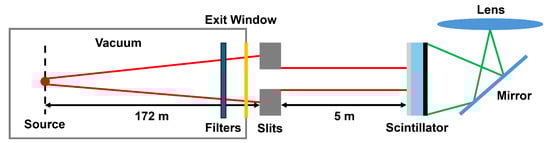
Figure 1. Schematic measurement setup. The source generates the extremely bright X-ray beam, which travels 172 m through a vacuum tube and attenuation filters. Behind the vacuum exit window, a two-axis collimator defines the X-ray beam. The detector (LCID) is positioned 5 m downstream of these quinary slits and uses an exchangeable scintillator that converts X-rays to optical photons. The latter are detected by a sCMOS camera and a lens.

In the present case, the detector is at $5\mathrm{m}$ downstream of the quinary slits, which act as the object that is imaged by the detector screen. The detector design is a lens-coupled indirect detector (LCID) with a $2\mathrm{mm}$ thick LuAG crystalline scintillator screen coupled to an 15 Megapixel ($5056\times 2968$) IRIS-15 sCMOS camera (Teledyne Photometrics, Tucson, AZ 85706, USA) with a 73% peak quantum efficiency and $4.25\mathsf{\mu }\mathrm{m}$ pixel pitch. The lens was a single f4/120 mm Hasselblad macro plana lens. All images were recorded with a sampling of $14.84\mathsf{\mu }\mathrm{m}$ in object (quinary slit) coordinates. The FoV covers $47\times 11.8{\mathrm{mm}}^2$ on the detector screen.

The measurements were each performed with four LuAG scintillators with different coatings. The first scintillator is the reference scintillator with the size of $55\times 85\mathrm{mm}$ and has no coating on the front (beam direction) or back (camera direction). The other scintillators are $35\times 50\mathrm{mm}$ and have an anti-reflection coating (AR) of ${\mathrm{SiO}}_2$ with 0.5% reflectance at a $535\mathrm{nm}$ wavelength ($100\mathrm{nm}$ FWHM) on the back. The AR coating was applied to the polished back surface using electron-beam physical vapor deposition. In order to measure the effects of AR coating, the front side of one of the scintillators was not coated. The remaining two had a reflective (R) coating or black (B) coating on the front. For the reflective coating, the front surface was optically polished and then coated with a reflective aluminum (Al) coating and a protective ${\mathrm{SiO}}_2$ coating, resulting in reflectance above 90% at a $535\mathrm{nm}$ wavelength [15,16]. The Al layer was deposited with a physical vapor deposition and had a thickness of about $100\mathrm{nm}$ to $150\mathrm{nm}$. Afterwards, 80 to $100\mathrm{nm}$ ${\mathrm{SiO}}_2$ was applied by Electron Beam Physical Vapor Deposition (EB-PVD). For the black coating, the front of the last scintillator was roughened 0.1–0.2$\mathsf{\mu }\mathrm{m}$ with sandpaper and then sprayed with a black graphite-based optical paint with high expected absorption.

For the uncoated reference scintillator, the FoV was $60.7\times 11.8{\mathrm{mm}}^2$. Note that the edges of the collimator blades were not directly aligned to the direction of propagation of the beam. A wedge of about $1^{\circ }$ made the edges free of phase contrast in the images. In the following, the scintillator screens are labeled with the abbreviation of the coating on the front and back. For example, the uncoated reference screen is labeled No/No.

With the beam limited by the slits to the full FoV of the R/AR scintillator screen, all intensities were recorded with an exposure time of $20\mathrm{ms}$ an average of 50 times. The electron ring had a current of $195\mathrm{mA}$ in a 7/8 multibunch mode, and the average beam energy was $106.4\mathrm{keV}$. The intensity distribution of the beam at the detector plane along the horizontal and vertical axes of the detector pixels is shown in Figure 2. Note that these profiles were taken from a fully illuminated detector image and include the scattered intensities that are examined by this study.

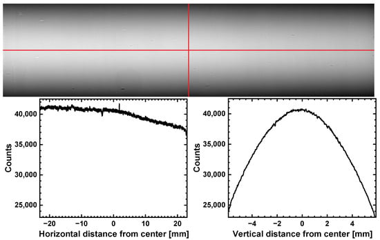
Figure 2. The projection and intensities across horizontal (left) and vertical (right) beam axes with an R/AR scintillator. The red lines show the used pixel for the line profiles. The beam is converted to optical photons by the R/AR scintillator while the collimator is fully open ($47\mathrm{mm}\times 11.8\mathrm{mm}$ at a $195\mathrm{mA}$ beam current and an average energy of $106.4\mathrm{keV}$).

2.2. Scattering

2.2.1. Theory

In the scintillator, an absorbed X-ray generates a burst of optical photons (cf. Figure 3). These primary photons are either directly or indirectly (after reflection on the front side) collected by the lens. The resulting counts are defined as the primary image $I_0$.

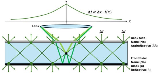
Figure 3. Schematic representation of photon generation and detection in the scintillator. An X-ray photon, indicated by the black spot in the scintillator, is converted into visible light. The visible photons are either directly detected by the lens (light green) or after the reflection at the front surface (green). Scattering occurs at the interfaces (dark green), where each scattering event leads to a loss of intensity $\Delta N$, which is also detected. Due to this attenuation, an exponential decay along the length of the scintillator (x) can be assumed (see the graph above). To influence the scattered light, the front side of the scintillator was either not coated (No) or coated in black (B) or a reflective layer (R). Meanwhile, the back side was either uncoated (No) or had an anti-reflective coat (AR).

In addition to the primary image, we expect scattered photons traveling between the two faces of the screen. With every bounce on the back or front side, some scattered photons are transmitted ($\Delta I$). One portion of the decreasing scattered intensity is, thus, collected by a camera and lens while the rest travels further. With this incremental loss, $\Delta I$ proportional to the intensity $I\left(x\right)$ and the path increment $\Delta x$; an exponential spread across the scintillator can be assumed. In summary, the following relationship can be defined for the scattered intensity $I_{scatt}$ along the scintillator length x:

$$\begin{array}{c}\hfill \Delta I\propto \Delta x·I\left(x\right)\to I_{scatt}\left(x\right)=c·I_0·exp\left(-{\displaystyle \frac{\left|x\right|}{d_{scat}}}\right)\end{array}$$

(1)

In order to distinguish scattered intensity from the primary image, we assume a constant portion c of the primary light is scattered. The scattering length $d_{scat}$ is a parameter for the spread of the scattered light. A higher value of $d_{scat}$ indicates a greater reach of the light scattering. Note that c as well as the scattering length $d_{scat}$ will most likely depend on the transmission/reflectivity of the front and back faces of the screens.

During conversion by the scintillator screen, we consider the X-ray image $I_0(x,y)$ to split into a sum of two images, both obtained by separate convolution kernels:

$$\begin{array}{c}\hfill I(x,y)=I_0(x,y)\ast \left[c·h_{\mathrm{scat}}(x,y)+h_{\mathrm{PSF}}(x,y)\right]\end{array}$$

(2)

$$\begin{array}{c}\hfill \mathrm{with}{h}_{\mathrm{scat}}(x,y)={\displaystyle \frac{1}{2d_{\mathrm{scat}}}}exp\left(-{\displaystyle \frac{\sqrt{x^2+y^2}}{d_{\mathrm{scat}}}}\right)\mathrm{and}c\in [0,1]\end{array}$$

(3)

On synchrotron beamlines, $h_{\mathrm{PSF}}$ is primarily defined by the optical blur of the LCID, i.e., by the aperture diffraction and limited depth of focus of the imaging lens [17]. Approximating the exponent in Equation (3) by its first-order Taylor terms yields the following:

$$\begin{array}{c}\hfill \sqrt{x^2+y^2}\approx \left|x\right|+\left|y\right|-{\displaystyle \frac{\left|x\right|\left|y\right|}{\left|x\right|+\left|y\right|}}=\left\{\begin{array}{cc}\left|x\right|& \mathrm{for}y\ll x\\ \left|y\right|& \mathrm{for}x\ll y\\ \left|x\right|+\left|y\right|& \mathrm{for}x,y\ll 1\end{array}\right\}\end{array}$$

(4)

$$\begin{array}{c}\hfill \mathrm{hence}{h}_{\mathrm{scat}}(x,y)\approx {\displaystyle \frac{1}{2d_{\mathrm{scat}}}}\left(e^{-{\displaystyle \frac{\left|x\right|}{d_{\mathrm{scat}}}}}·e^{-{\displaystyle \frac{\left|y\right|}{d_{\mathrm{scat}}}}}·e^{{\displaystyle \frac{1}{d_{\mathrm{scat}}}}{\displaystyle \frac{\left|x\right|\left|y\right|}{\left|x\right|+\left|y\right|}}}\right)\end{array}$$

(5)

Convoluting a rectangular aperture $W(x,y)$ with horizontal and vertical openings $g_H$ and $g_V$, respectively, with $h_{\mathrm{scat}}$ from Equation (5) simply yields the convolution of the unscattered intensity $I_0(x,y)$ with the integral bounds W:

$$\begin{array}{c}\hfill I_{\mathrm{scat}}(x,y)\approx c·{\int \int }_W{I}_0\left(x^{\prime },y^{\prime }\right)·h_{\mathrm{scat}}(x-x^{\prime },y-y^{\prime })d{x}^{\prime }d{y}^{\prime }\end{array}$$

(6)

2.2.2. Hgap Experiment

In this first setting, the two-axis quinary slit system of BM18 is used to shape a rectangular aperture with constant vertical opening $g_V=12$ mm and variable horizontal opening $g_H$ increasing from 5 mm to 50 mm by steps of 5 mm. Intensity is evaluated at the image center, $W(x,y)$, while assuming $I_0(x,y)=I_0$ in this region. If $g_V>d_{\mathrm{scat}}$, it is justified to consider only convolution in x and put all terms in Equation (5) that depend on y into a factor $c_H$:

$$\begin{array}{c}\hfill \begin{array}{cc}\hfill I_{\mathrm{hgap}}\left(g_H\right)& =I_0+c_H·I_0{\int }_{{\displaystyle \frac{-g_H}{2}}}^{{\displaystyle \frac{g_H}{2}}}exp\left(-{\displaystyle \frac{\left|x\right|}{d_{scat,H}}}\right)dx\hfill \\ \hfill & =I_0+2·c_H·I_0·d_{Scat,H}·\left(1-exp\left(-{\displaystyle \frac{g_H}{2·d_{Scat,H}}}\right)\right)\hfill \\ \hfill & =\left(I_0+2·c_H·I_0·d_{Scat,H}\right)-2·c_H·I_0·d_{Scat,H}·exp\left(-{\displaystyle \frac{g_H}{2·d_{Scat,H}}}\right)\hfill \\ \hfill & =I_{0,H}-I_{\mathrm{S}\mathrm{c}\mathrm{a}\mathrm{t}\mathrm{,}\mathrm{H}}·exp\left(-{\displaystyle \frac{g_H}{2·d_{Scat,H}}}\right)\hfill \end{array}\end{array}$$

(7)

The resulting curve is again a growing exponential, defined by the length $d_{scat,H}$, which does not necessarily equal $d_{scat}$ from (s. Appendix A.1). The experimental procedure is shown schematically in Figure 4 (left). Average detector count rates in a square of $25\times 25$ pixels at the center of $W(x,y)$ are evaluated as a function of $g_H$ using Equation (7) as a fitting function.

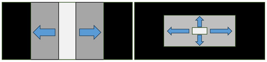
Figure 4. Schematic representation of the hgap (left) and rect measurement procedures (right). The arrows indicate the movement of the slits.

2.2.3. Rect Experiment

In a second experimental setting, W(x,y) was used to define a rectangular window of constant ratio $g_H/g_V=5$ and increasing area. The initial area of the window was $1\mathrm{mm}\times 5\mathrm{mm}$. Step-wise enlarging $g_H$ by $5\mathrm{mm}$, therefore, leads to enlarging $g_V$ by $1\mathrm{mm}$ with each step. This experimental procedure is shown schematically in Figure 4 (right).

Normalizing the measured detector count rate $I_{\mathrm{rect}}(g_H,g_V)$ with respect to $I_{\mathrm{hgap}}\left(g_H\right)$ for the same values of $g_H$ in the previous experiment should approximate the scattering contribution in the vertical direction. Assuming that horizontal and vertical contributions factorize in this setting, the ratio $R_V=I_{\mathrm{rect}}/I_{\mathrm{hgap}}$ would fit an exponentially growing function, which would be unity at $g_V=12$ mm. As a result, $R_V$ as a function of $g_V$ becomes

$$\begin{array}{c}\hfill R_V\left(g_V\right)={\displaystyle \frac{I_{rect}}{I_{hgap}}}=1-I_{Gain,V}·exp\left(-{\displaystyle \frac{g_V}{d_{\mathrm{s}\mathrm{c}\mathrm{a}\mathrm{t}\mathrm{,}\mathrm{V}}}}\right)\end{array}$$

(8)

Note that the condition that $R_V$ converges to unity is motivated by the steep intensity drop in the vertical beam direction (cf. Figure 2). After subtracting scattered light, there is hardly any beam intensity beyond $g_V=12$ mm.

2.3. Modulation Transfer Function

Modulation transfer (MTF or $H(u_x,u_y)$) is the absolute value of the 2D Fourier transform of the system’s point spread function (PSF or $h(x,y)$). The latter is commonly approximated by the line spread function (LSF) measured across an opaque knife edge in the image. Here, we must deviate from this concept since, obviously, h includes the optical scattering inside the scintillator according to Equation (2).

$$\begin{array}{c}\hfill H\left(u\right)=H_{\mathrm{scat}}\left(u\right)+H_{\mathrm{PSF}}\left(u\right)\end{array}$$

(9)

The contribution $H_{\mathrm{PSF}}$ is the Fourier transform of $h_{\mathrm{PSF}}$ while $H_{\mathrm{scat}}$ represents the optical scattering of interest. For the sake of simplicity, we only consider the radial component of h and H by writing $u=\sqrt{u_x^2+u_y^2}$. While disentangling $h_{\mathrm{scat}}$ and $h_{\mathrm{PSF}}$ in real space is only possible if one of these two is precisely known, one might succeed in obtaining $H_{\mathrm{scat}}$ and $H_{\mathrm{PSF}}$ simultaneously if both contributions are confined in separate frequency bands. If $d_{\mathrm{scat}}\gg {\sigma }_{\mathrm{PSF}}$, then $H_{\mathrm{scat}}$ will only show in the low-frequency band where $H_{\mathrm{PSF}}$ is unity. The latter will solely constitute the higher frequencies where $H_{\mathrm{scat}}=0$.

For measuring the convolution kernel, one vertical blade of the quinary slit system was set in the middle of the detector, covering half its FoV. The sum of three Gaussian functions is used to model $H_{PSF}\left(u\right)$:

$$\begin{array}{c}\hfill H_{PSF}\left(u\right)=\sum _{n=1}^3{A}_{n}exp\left(-2{\pi }^2·{\sigma }_n^2·u^2\right)\end{array}$$

(10)

For practical reasons the measured $H\left(u\right)$ is first fitted to Equation (10) by eclipsing low frequencies below $\left|u\right|<0.2$ LP/mm. The resulting fit is subtracted from $H\left(u\right)$, and the residual is fitted to a Lorentzian function, i.e., the Fourier transform of an exponential:

$$\begin{array}{c}\hfill H_{\mathrm{scat}}\left(u_x\right)=\mathcal{F}\left[A·exp\left(-{\displaystyle \frac{\left|x\right|}{d_{\mathrm{M}\mathrm{T}\mathrm{F}\mathrm{,}\mathrm{s}\mathrm{c}\mathrm{a}\mathrm{t}}}}\right)\right]={\displaystyle \frac{A}{u_x^2+\frac{1}{d_{\mathrm{M}\mathrm{T}\mathrm{F}\mathrm{,}\mathrm{s}\mathrm{c}\mathrm{a}\mathrm{t}}^2}}}\end{array}$$

(11)

Here, A stands for the amplitude of $H_{Scat}$, i.e., the strength of the scattering component in the signal. Note that the standard deviation $\sigma$ of a 2D Gaussian does not change when the latter is projected vertically, i.e., when LSF is measured instead of PSF and fitted to a 1D Gaussian. The same is not true for a 2D exponential (cf. Equation (1)):

$$\begin{array}{c}\hfill h_{\mathrm{s}\mathrm{c}\mathrm{a}\mathrm{t}\mathrm{,}\mathrm{L}\mathrm{S}\mathrm{F}}\left(x\right)={\int }_{-\infty }^{\infty }{h}_{\mathrm{scat}}(x,y)dy={\int }_{-\infty }^{\infty }exp\left(-{\displaystyle \frac{\sqrt{x^2+y^2}}{d_{scat}}}\right)dy\end{array}$$

(12)

Despite not having an analytical expression for $h_{\mathrm{s}\mathrm{c}\mathrm{a}\mathrm{t}\mathrm{,}\mathrm{L}\mathrm{S}\mathrm{F}}\left(x\right)$, it is obviously not an exponential. Fortunately, the Lorentzian from Equation (11) remains a good approximation of its Fourier transform $h_{\mathrm{s}\mathrm{c}\mathrm{a}\mathrm{t}\mathrm{,}\mathrm{L}\mathrm{S}\mathrm{F}}\left(u_x\right)$ with significant deviations only in the functions’ tails (cf. Appendix A.2). Consequently, one has to keep in mind that $d_{\mathrm{s}\mathrm{c}\mathrm{a}\mathrm{t}\mathrm{,}\mathrm{L}\mathrm{S}\mathrm{F}}\ne d_{\mathrm{scat}}$, i.e., a factor $1.385$ has to be applied for upscaling $h_{\mathrm{s}\mathrm{c}\mathrm{a}\mathrm{t}\mathrm{,}\mathrm{L}\mathrm{S}\mathrm{F}}$.

3. Results

3.1. Hgap Experiment

Figure 5 shows the measured count rates for the four different scintillator coatings as a horizontal line profile along the equator of $W(x,y)$. The horizontal opening of the latter was $5\mathrm{mm}$ (lined) and $25\mathrm{mm}$ (dashed), while $g_V=12$ mm was constantly open.

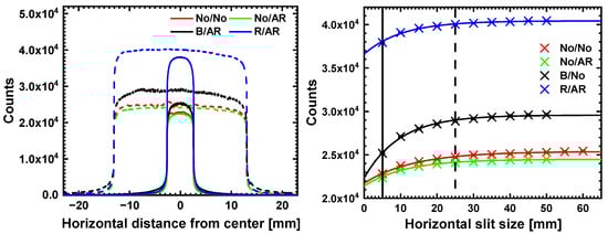
Figure 5. Left: Measured counts of the four scintillators with different coatings along the horizontal axis for slit sizes of $5\mathrm{mm}$ (solid line) and $25\mathrm{mm}$ (dashed line). Right: Averaged counts at the center plotted against the slit size. The positions of the measurements displayed on the left are marked by solid and dashed lines. The values were fitted using Equation (7).

The scintillator with a reflective coating (R/AR) visibly yields higher count rates, whereas the black coating (B/AR) shows moderately higher count rates compared to No/No and No/AR, which are similar in that respect. Furthermore, a larger horizontal opening yields higher count rates for all scintillator coatings because an increasingly large amount of scattered light is collected. This contribution from optical scattering would be maximum if the entire screen were illuminated by X-rays. The ratios of count rates among the coatings persists when $g_H$ is raised, with a minor exception: No/No shows a faintly higher rate compared to No/AR while the opposite is observed for $g_H=5$ mm.

In order to test Equation (7), the average counts at the center of $W(x,y)$ were plotted as a function of $g_H$ (cf. Figure 5). Equation (7) was fitted to this data, yielding the fit parameters $d_{\mathrm{s}\mathrm{c}\mathrm{a}\mathrm{t}\mathrm{,}\mathrm{H}}$, $I_{0,H}$ and $I_{\mathrm{s}\mathrm{c}\mathrm{a}\mathrm{t}\mathrm{,}\mathrm{H}}$. These numbers as well as their confidence bounds are displayed for all scintillators in Table 1. From the result we computed $I_H(g_H=0)$ as well as $c_{\mathrm{S}\mathrm{c}\mathrm{a}\mathrm{t}\mathrm{,}\mathrm{H}}$, i.e., the ratio between $I_{\mathrm{s}\mathrm{c}\mathrm{a}\mathrm{t}\mathrm{,}\mathrm{H}}$ and $I_H(g_H=0)$, the strength of the scattered light with respect to the unscattered light.Both $d_{\mathrm{s}\mathrm{c}\mathrm{a}\mathrm{t}\mathrm{,}\mathrm{H}}$ and $c_{\mathrm{s}\mathrm{c}\mathrm{a}\mathrm{t}\mathrm{,}\mathrm{H}}$ were corrected through comparison with analytical simulations to approximate the actual $d_{\mathrm{Scat}}$ and c from Equation (1) (cf. Appendix A). The corrected values $d_{\mathrm{scat},\mathrm{H}}^{\prime }$ and $c_{\mathrm{scat},\mathrm{H}}^{\prime }$ can also be found in Table 1.

Table 1. Results from fitting an exponential law to the hgap data. Fit parameters according to Equation (7) are $d_{\mathrm{scat}\mathrm{,}\mathrm{H}}$ and the relative portion of scattering counts $c_{\mathrm{scat},\mathrm{H}}$ from Figure 5 (right). $d_{\mathrm{scat}}^{\prime }$ and $c_{\mathrm{scat},\mathrm{H}}^{\prime }$ are the corrected values obtained through numerical simulations (cf. Appendix A).

	No/No	No/AR	B/AR	R/AR
$I_H(g_H\to \infty )$	25,379$\pm 47$	24,482$\pm 41$	29,572$\pm 69$	40,420$\pm 49$
$I_{Scat,H}$	$3647\pm 93$	$3077\pm 202$	$7230\pm 220$	$3821\pm 267$
$I_H(g_H=0)$	21,732$\pm 104$	21,404$\pm 206$	22,342$\pm 231$	36,600$\pm 272$
$c_{\mathrm{Scat},\mathrm{H}}$	$0.1678\pm 0.0051$	$0.144\pm 0.011$	$0.324\pm 0.014$	$0.104\pm 0.083$
$d_{Scat,H}\left[\mathrm{mm}\right]$	$6.81\pm 0.44$	$5.7\pm 0.5$	$4.90\pm 0.28$	$5.19\pm 0.48$
$c_{\mathrm{scat},\mathrm{H}}^{\prime }$	$0.432\pm 0.013$	$0.319\pm 0.024$	$0.634\pm 0.027$	$0.213\pm 0.017$
$d_{\mathrm{scat}}^{\prime }\left[\mathrm{mm}\right]$	$6.10\pm 0.39$	$4.99\pm 0.43$	$4.20\pm 0.24$	$4.48\pm 0.41$

The uncoated (No/No) and the AR backside-coated (No/AR) scintillators seem to yield the same amount of unscattered light: 21,732 vs. 21,404 counts, respectively. Yet, the uncoated scintillator displays a $20\%$ higher amount of scattered light: 3647 vs. 3077. The corrected ratios $c_{\mathrm{Scat},\mathrm{H}}^{\prime }$ for the uncoated and the No/AR screens are $43.2\%$ and $31.9\%$, respectively. Additional reflective front-coating (R/AR) produces a $71\%$ higher rate of unscattered light (36,600 counts). Meanwhile, the amount of scattered intensity is only faintly larger than the uncoated scintillator, making R/AR the screen with the lowest count ratio ($21.3\%$ after correction). Grinding and coating the front side with black paint (B/AR) yields a faint increase in $I_H(g_H=0)$ (22,342) while scattered intensity doubles (7230) with respect to the uncoated screen. The ratio $c_{\mathrm{Scat},\mathrm{H}}^{\prime }$ for B/AR is $63.4\%$, i.e., twice as high as No/AR and thrice as high as R/AR.

Regarding scattering length $d_{\mathrm{Scat},\mathrm{H}}^{\prime }$, B/AR displays the shortest ($4.2$ mm) while the uncoated screen has the longest value ($6.1$ mm). The No/AR and R/AR screens have intermediate values: $4.99$ mm and $4.48$ mm, respectively.

3.2. Rect Experiment

During this experiment the vertical opening of W increased alongside $g_H$, whereby the ratio $g_H/g_V=5$ was constant. Figure 6 displays horizontal intensity profiles for the four different scintillator coatings at $(g_H,g_V)=(5$ mm,$1$ mm) as well as (25 mm,$5$ mm). Regarding intensity ratios, the observations from the hgap experiment are confirmed with one notable exception: the (5 mm,$1$ mm) opening sets all coatings at the same count rate (≈20,000) except for R/AR, which displays ≈34,000 counts, hence a $70\%$ higher value.

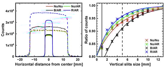
Figure 6. Left: Measured counts for all four scintillators along the horizontal axis for pinhole sizes of $1\times 5\mathrm{mm}$ (solid line) and $5\times 25\mathrm{mm}$ (dashed line). Right: Ratio of the counts at the center of Figure 6 (left) to Figure 5 (left) plotted against the vertical slit size. The positions of the measurements displayed on the left are marked by solid and dashed lines. The values were fitted using Equation (8).

This observation is in strong contrast to the graph that displays the ratio $R_V\left(g_V\right)$ (cf. Equation (8)) of the rect with respect to the hgap intensities at matching horizontal openings $g_H$ as a function of $g_V$. The profiles for No/No, No/AR, and R/AR converge towards $0.8$ at $g_V=0$. The ratio for the B/AR coating, however, deviates significantly from the other three: when the vertical gap closes, the drop in terms of count rate is much more significant for B/AR.

Toward $g_V=12$ mm, all four profiles converge to unity, confirming the assumption of a quasi-zero beam intensity beyond this window size. Fitting these profiles to Equation (8) yields estimates for $I_{\mathrm{Gain},\mathrm{V}}$ as well as $d_{\mathrm{Scat},\mathrm{V}}$. The latter is corrected trough analytical simulations yielding $d_{\mathrm{Scat},\mathrm{V}}^{\prime }$, which approximates the actual scatter length from Equation (1) (see Table 2).

Table 2. Resulting fit parameters according Equation (8) from Figure 6 (right).

	No/No	No/AR	B/AR	R/AR
$I_{Gain,V}$	$0.1961\pm 0.0083$	$0.1979\pm 0.0091$	$0.2892\pm 0.0055$	$0.196\pm 0.015$
$d_{scat,V}\left[\mathrm{mm}\right]$	$2.19\pm 0.14$	$1.836\pm 0.089$	$2.097\pm 0.069$	$1.58\pm 0.13$
$d_{scat,V}^{\prime }\left[\mathrm{mm}\right]$	$3.36\pm 0.21$	$3.31\pm 0.16$	$3.26\pm 0.11$	$3.86\pm 0.32$

All values $d_{\mathrm{Scat},\mathrm{V}}^{\prime }$ fall short of $d_{\mathrm{Scat},\mathrm{H}}^{\prime }$, which is shown in Table 1. While B/AR still features the shortest scattering length ($3.26$ mm), the highest value is now obtained for R/AR: $3.86$ mm with intermediate values for No/No and No/AR. The values of $I_{Gain,V}$ all coincide with the ratio $g_V/g_H=0.2$, except for B/AR, which features $I_{Gain,V}=0.289$.

3.3. Modulation Transfer Function

One vertical blade from the quinary slits was positioned on one side at the beam center to measure the LSF. Meanwhile, the vertical opening was constantly $g_V=12$ mm. The resulting horizontal line profiles that were obtained from transmission images of the edge on the different screens are shown in Figure 7 on a linear as well as on a normalized semi-log scale. The net difference in count rates from the four screens as it was measured by the hgap and rect experiments defines the bright side of the profile, while the scattered portion of the light and its exponential decrease away from the edge feature on the dark side, i.e., in the shadow of the blade.

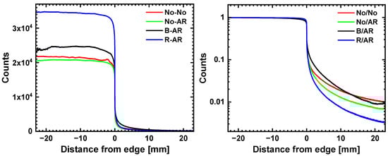
Figure 7. Left: Measured counts at the center with a $20\mathrm{mm}$ thick tungsten edge for the four different scintillators. Right: Normalized transmissions in the shadow of the blade.

Similarly to hgap, R/AR displays the highest count rate (34,465), followed by B/AR (24,606), while No/AR and No/No feature similarly low rates: 20,722 and 21,712, respectively. For the semi-log display of the scattered portion of these bright count rates, the profiles are normalized with respect to the latter. Figure 7 (right) reveals stark differences in the relative amount of scattered light (area covered by the dark side of the line profiles) for the different screen coatings. While No/No and B/AR appear to have the highest amount of scattered light, the rates at which the latter decreases away from the edge differ a lot (B/AR starts with a higher amount but decreases faster). Meanwhile, No/AR and R/AR show a similarly slow decrease, yet the relative amount of scattered light is visibly less for No/AR and a lot less for R/AR with respect to the No/No screen.

These qualitative results are corroborated by quantitative estimates of $H\left(u\right)$. To obtain the latter, LSF was calculated by differentiating and then Fourier-transforming the normalized line profiles in Figure 7 with respect to x. The resulting 1D MTF of the No/No screen is displayed in Figure 8 along with function fits for $H_{\mathrm{PSF}}$ and $H_{\mathrm{Scat}}$, which were computed in this order. The part of the spectrum with $\left|u\right|<0.2$ LP/mm was eclipsed for fitting $H_{\mathrm{PSF}}$ with the sum of three Gaussians; then, the resulting fit was subtracted from $H\left(u\right)$ to fit $H_{\mathrm{Scat}}$ (again for $\left|u\right|<0.2$ LP/mm) with a Lorentzian.

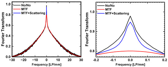
Figure 8. Left: Determined $H\left(u\right)$ of No/No with the $H\left(u\right)$ fit, both with and without scattering. Right: Low frequency range of MTF ($\left|u\right|<0.2$ LP/mm) with a Lorentzian fit for the uncoated screen.

The fitting parameters of $H_{\mathrm{PSF}}$ were very similar for all four scintillators. All scintillator screens had a thickness of $2\mathrm{mm}$, and Diez et al. showed that different coatings had a little effect on the MTF [18]. Rather, the dominant factor influencing resolution was the lens used, which was identical in all cases. In this study, $H_{\mathrm{PSF}}$ is not the focus of the investigation and is, therefore, not considered in further detail.

The relative magnitude and range of $H_{\mathrm{Scat}}$ reflect the relative portion of scattered light in the screens. Note that $d_{\mathrm{Scat}}$ had to be multiplied with a factor of $1.385$ to correct for the difference between 1D and 2D Fourier transforms of the exponential $h_{\mathrm{Scat}}(x,y)$ (cf. Equation (3)). The resulting fit parameters from Equation (11) as well as the corrected scattering length $d_{\mathrm{Scat}}^{\mathrm{LSF}}$ are listed in Table 3 for the four screen coatings.

Table 3. Resulting fit parameters according to Equation (11) from Figure 8. The last line shows corrected values of $d_{\mathrm{scat}}$ estimated from fitting LSF measures to Lorentzian peaks (normalization factor $1.385$).

	No/No	No/AR	B/AR	R/AR
A	$0.1479\pm 0.0049$	$0.153\pm 0.017$	$0.2464\pm 0.0082$	$0.1248\pm 0.0082$
$d_{scat}$ [mm]	$4.18\pm 0.29$	$3.23\pm 0.61$	$4.13\pm 0.28$	$3.15\pm 0.36$
$d_{\mathrm{scat}}^{\mathrm{LSF}}\left[\mathrm{mm}\right]$	$4.74\pm 0.34$	$3.65\pm 0.65$	$4.68\pm 0.32$	$3.57\pm 0.40$

In agreement with the hgap and rect experiments, the B/AR coating produces the highest amount of scattered light (A; hence, the zero-frequency amplitude of $H_{\mathrm{Scat}}\left(u\right)$ with respect to $H\left(u\right)$ in Figure 8), i.e., $A=0.2464$, while R/AR yields less than half this value: $0.1248$. The uncoated screen No/No and the No/AR backside-coated screen feature intermediate values of $A=0.1479$ and $A=0.153$, respectively. After correction, $d_{\mathrm{Scat}}^{\mathrm{LSF}}$ is almost equal for No/No and B/AR with $4.74$ mm and $4.68$ mm, respectively, while shorter scattering lengths are obtained for No/AR and R/AR: $3.65$ mm and $3.57$ mm, respectively.

4. Discussion

4.1. Measurements Method

The present study compares three experimental routes for measuring the optical scattering inside transparent crystalline scintillator screens by using a two-dimensional slit collimator. Opening the horizontal gap step-wise, with the vertical gap open, yields an increasing intensity that fits to a limited exponential growth (hgap). Simultaneously, first closing then opening the vertical gap stepwise while keeping the ratio $g_H/g_V=5$ constant and normalizing intensity to the value from the same horizontal opening in hgap yields an intensity ratio that also fits a similar exponential law (rect).

We assume that the observed intensities are convolutions of the collimator window with a radially symmetric exponential kernel. To deduce the amplitude c and scattering length $d_{\mathrm{scat}}$ from the fitting exponential’s parameters, we recreated the convolution numerically by using similar parameters for $d_{\mathrm{scat}}$ and for the beam intensity profile.

In the hgap experiment, the horizontal slit was opened step-wise up to the horizontal size of the field-of-view, i.e., $47\mathrm{mm}$ (note: the horizontal size of the No/No screen was $85\mathrm{mm}$, whereas the other screens were $50\mathrm{mm}$ wide). Fitting an exponential law to the measured intensities produced a good match whereby different levels of saturation (in units of counts) were reached for each screen.

While for the hgap and the rect experiments the scattered intensity as a function of the slit openings is not described by an analytical formula (cf. Equation (5)), numerical simulations are able to perform the convolution explicitly and obtain the ground truth for matching fitting parameters of the experimental results ($d_{\mathrm{scat},\mathrm{H}}$) to the actual values of $d_{\mathrm{scat}}$ and c (cf. Appendix A.1). For hgap, the simulations predict a downscaling of $d_{\mathrm{scat},\mathrm{H}}$ as well as an upscaling of c, e.g., $d_{\mathrm{scat},\mathrm{H}}=5.19\mathrm{mm}$ for R/AR coating, which becomes $4.48\mathrm{mm}$ after correction. Likewise, for the same screen, the proportion of the scattered light with respect to the unscattered intensity is measured $0.104$ but becomes $0.213$ after correction. Despite these differences, all measurement data fitted well to the exponential model with confidence bands in the range of 5–10%.

In the rect experiment, we used the results of hgap to normalize the measured count rates when the slits were additionally closed in the vertical direction with a constant aspect ratio $g_H/g_V=5$. These resulting normalized intensities could be fitted to an exponential law that was also reproduced in the simulations, allowing for a similar correction of the observed values of $d_{\mathrm{scat},\mathrm{V}}$.

However, the resulting scattering lengths were significantly shorter than those observed by hgap, e.g., $3.86\mathrm{mm}$ for rect vs. $4.48\mathrm{mm}$ for hgap. Note that in the simulations we included a strong vertical drop in primary intensity from the beam center to the vertical edge of the field-of-view to mimic the experimentally observed beam profile (cf. Figure 2). However, in order to achieve a good match in the normalized intensities (cf. Figure 6) between the rect experiment and simulations, an assumption was made regarding the portion of scattered light in the recorded beam profile.

For rect, these corrections led to a significant upscaling of $d_{\mathrm{scat},\mathrm{V}}$, e.g., $d_{scat,V}=1.58\mathrm{mm}$ for R/AR coating was corrected to $d_{\mathrm{scat}}=3.86\mathrm{mm}$. Yet, even after correction, all scattering lengths stayed short of the values from the hgap experiment.

In the last method, we calculated MTF by Fourier-transforming the line spread function (LSF) as it was measured across a single blade of the collimator. In order to obtain the shape and portion of scattered light from the MTF, our analysis assumed a clear separation of these two components in the spatial frequency domain, i.e., the scattering MTF is confined to a very low frequency band where the image blur yields only a constant offset.

The resulting fit (Lorentzian, after subtraction of the offset and restriction to frequencies between $\pm 0.2\mathrm{LP}/\mathrm{mm}$) yielded another estimate of $d_{\mathrm{scat}}$ that was upscaled by a factor 1.385. The latter was obtained from calculating the convolution of a radial exponential kernel with a line and fitting the Lorentzian to its Fourier transform (cf. Appendix A.2).

The data, however, indicates that the assumption of the frequency bands for blur and scatter MTF perfectly separating is only partly valid and the shape of the presumably scattering MTF peak only matches the Lorentzian at its center and not in the tails of the MTF. One obvious result of this limited validity is that the MTF analysis estimates dscat of B/AR coating to be similar to the other screens ($4.68\mathrm{mm}$ and $4.74\mathrm{mm}$), even though the edge intensity profile (Figure 7) indicates a visibly steeper slope for B/AR.

Nevertheless, the resulting estimates of $d_{\mathrm{scat}}$ lie remarkably close to the value of hgap and rect, e.g., $3.57\mathrm{mm}$ for R/AR coating. We estimated the portion of scattered light by comparing the amplitude of the scatter MTF while setting the maximum of the combined MTF to unity. These values are similar but generally smaller than the estimates of scattering light fractions from hgap.

4.2. Potential Error Sources

Transmission images (hgap, rect, and LSF for each screen) were recorded in relatively quick acquisition sequences. During one sequence the synchrotron ring current ($195\mathrm{mA}$) did not change significantly. Therefore, the count rates constitute an absolute scale for each sequence. The hgap as well as the rect experiment sequences each began with the quinary slits closed. The latter were opened increasingly step by step, horizontally for hgap and area-wise for rect. If the intense synchrotron beam was to cause a bright burn or strong remanence in the scintillator, the newly illuminated areas would appear darker than the rest of the bright field. Such an effect was not observed from the present data. It can, therefore, be assumed that the measured intensities either represent the primary image or the scattered light.

While simulations helped in correcting errors made by assuming the factorization of horizontal and vertical scatter components in Equation (1), the underlying model ignored the edges of the scintillators. At least in the horizontal direction, the latter were not far from the edges of the FoV, possibly affecting the recorded intensities, e.g., by reflecting scattered light on their blunt uncoated surfaces.

Regarding the converted X-rays, a higher mean photon energy yields more optical photons. However, the Compton scattering of X-rays at very high energies will likely add an image blur to the primary intensities, which will depend on the screen thickness. For the $106\mathrm{keV}$ mean energy of this study, we can assume that Compton scattering is negligible, and attenuation in the screen is purely due to the photoelectric effect.

4.3. Differences Between the Coatings

One of the scintillators had no coating at all. Here, the intention was to verify the assumption that coating the backside of transparent screens would reduce the total amount of scattered light by allowing the latter an easier exit through the backside of the screen. This assumption is strongly corroborated by the hgap experiment, which reveals a larger amount of scattered light in No/No with respect to No/AR (0.432 vs. 0.319 after corrections) as well as a larger scattering length ($6.10\mathrm{mm}$ vs. $4.99\mathrm{mm}$). The rect experiment is likely insensitive to the absolute portion of scattered light since it is already normalized with respect to hgap. Meanwhile, No/No and No/AR feature almost identical amplitudes in the MTF analysis (0.148 and 0.153) while this method still predicts the longest $d_{scat}$ for the uncoated scintillator ($4.74\mathrm{mm}$).

The black front coating B/AR was applied after roughening the front side of the screen to test whether such a coating would improve or worsen the scattering properties of the scintillator. From our observations it can clearly be concluded that the latter is the case. Most obviously, it yields a much higher portion of scattered light in the hgap experiment. In hgap and rect, B/AR also features the shortest values of $d_{scat}$, indicating that scattering is relatively stronger and shorter-ranged than in all other screens. The only exception is the MTF results, which feature a long scattering length ($4.68\mathrm{mm}$) that, however, is contradictory with the visual observation of the corresponding edge profile that clearly shows a steeper decrease (see above).

Diffuse scattering at the rough, blackened surface most likely causes these effects. At the same time, the blackened surface reduced the reflectivity of the front side, yielding a lesser portion of primary image intensity. This interpretation is corroborated by measurements of SNR power spectra that we recently published on the same coated screens [18].

The very large amount of scattered light in the images from the B/AR screen also shows in Figure 6 where B/AR has a higher count rate than No/No and No/AR for a large collimation ($5\times 25\mathrm{mm}$) while it has the same count rate for a small collimation ($1\times 5\mathrm{mm}$).

Meanwhile, the reflective coating generally improves the optical scattering effects in the R/AR screen by increasing the internal reflectivity of the front surface. The latter yields a significantly higher gain in primary intensity while it does not worsen the amount of scattered light with respect to the No/AR screen. In comparison to No/AR, R/AR yields approx. 90% more primary signals while the increase in scattered intensity is much less. This observation is corroborated by the SNR power spectra, which we recently published on the same screens [18].

We do not observe a significant difference in terms of scattering length between No/AR and R/AR. This indicates that $d_{scat}$ is mainly influenced by the AR backside coating (i.e., No/No features larger values of $d_{scat}$ compared to No/AR and R/AR) as well as by the black coating on the front of B/AR, which shows shorter values of $d_{scat}$.

We do not report on the estimates of $H_{PSF}$, which was fitted to a sum of Gaussians during the MTF analysis. This fit produced the same (primary) image sharpness for all four screens. This confirms previous results from the same screens that estimated MTF from line patterns [18].

5. Conclusions

5.1. Reliable Measurement of Optical Scattering

Regarding potential error sources, being the only direct measure, the hgap method appears relatively robust while the rect and MTF analyses depend more strongly on assumptions made by simulations. If the approximate value of $d_{\mathrm{scat}}$ had been known, using one image from a single round pinhole might have been sufficient. The diameter of the pinhole needs to be carefully chosen (larger than the PSF while much smaller than $d_{\mathrm{scat}}$; here, approx. $50 \mathsf{\mu }\mathrm{m}$ would be a good choice). However, for additionally estimating the relative portion c of scattered light, hgap appears to be the most reliable method.

Using these findings for correcting the scattered intensity prior to tomographic imaging (back projection) will likely yield significant improvements to the latter [13]. Even in the best case (R/AR), scattered light amounted to >20% of the unscattered intensity.

5.2. Benefits from Coated Scintillators

To summarize, a reflective coating on the front and an anti-reflective coating on the back turn out to be a good choice for scintillators. Both coatings reduce the effects of optical scattering and even increase the light output compared to other scintillators.

In terms of image quality, the R/AR coating clearly yields the best results. The primary signal is amplified by the reflective coating with no notable difference in image sharpness. Meanwhile, the amount of scattered light, which increases detector count without contributing to the actual signal, is only mildly greater than in the No/AR scintillator.

The application of the measurements in this study to the powder screens in laboratory flat-panel detectors may prove interesting, also with regard to possible coatings of these screens [19]. Optical scattering in these screens is different from transparent scintillator screens but causes similar problems/artifacts for tomographic imaging.

Appendix A.1

Considering Equation (3) valid, the scattering lengths $d_{\mathrm{scat},\mathrm{H}}$ and $d_{\mathrm{scat},\mathrm{V}}$ are bound to deviate from the actual value $d_{\mathrm{scat}}$ due to the entanglement of the vertical and horizontal components of the window formed by the pair of slits.

Recreating the scattered light image by means of numerical simulation is the easiest way to estimate and correct the measurements of $d_{\mathrm{scat},\mathrm{H}}$ and $d_{\mathrm{scat},\mathrm{V}}$. For each measurement step, a rectangular window $W(x,y)$ on a black background defines the slits’ aperture from the experiment of hgap or rect. Virtual images are ${\left(2000\right)}^2$ pixels and sampled with a pixel size of $\Delta x=0.05$ mm. W includes multiplication with a parabolic vertical intensity profile to reproduce the profile in Figure 2. The simulated scattered light is computed by convolving W with $h_{\mathrm{scat}}(x,y)$, cf. Equation (3):

$$\begin{array}{c}\hfill \begin{array}{c}\hfill I_{\mathrm{scat}}(x,y)=(W\ast h_{\mathrm{scat}})={\mathrm{FT}}^{-1}\left[\mathrm{FT}\left\{W\right\}·\mathrm{FT}\left\{h_{\mathrm{scat}}\right\}\right]\\ \hfill \mathrm{with}{h}_{\mathrm{scat}}(x,y)=h_{\mathrm{scat}}\left(r\right)={\displaystyle \frac{1}{2d_{\mathrm{scat}}}}exp\left(-{\displaystyle \frac{r}{d_{\mathrm{scat}}}}\right)\end{array}\end{array}$$

(A1)

assuming a radial exponential kernel with unit area and $r=\sqrt{x^2+y^2}$. Figure A1 displays the normalized intensities in the center of the window W after the convolution of the latter with $h_{\mathrm{scat}}(x,y)$ for a horizontal opening from 5 mm to 60 mm, $g_V=\mathrm{const}.=12$ mm and $d_{\mathrm{scat}}=6$ mm. Fitting an exponential (Equation (7)) to these values yields $d_{\mathrm{scat},\mathrm{H}}=6.71$ mm and $I_{\mathrm{scat},\mathrm{H}}=0.460$; hence, vertical clipping by the slits yields $46\%$ of the total scattered intensity.

Recreating the rect experiment, i.e., keeping the ratio of horizontal and vertical openings constantly 5:1 and normalizing the intensity with respect to hgap for the same horizontal openings, also produces an exponential that is unity for $(g_H,g_V)=(60\mathrm{mm},12\mathrm{mm})$. Curve fitting yields $d_{\mathrm{scat},\mathrm{V}}=2.85$ mm. Equivalent fits were produced by the same workflow for $d_{\mathrm{scat}}=5$ mm and $d_{\mathrm{scat}}=4$ mm, yielding estimates for $d_{\mathrm{scat},\mathrm{H}}$ and $d_{\mathrm{scat},\mathrm{V}}$ for these values (cf. Table A1). A quadratic polynomial $d_{\mathrm{scat}}^{\prime }=a+b·d_{\mathrm{scat},\mathrm{H}}+c·d_{\mathrm{scat},\mathrm{H}}^2$ was created from these results to estimate the correct length $d_{\mathrm{scat}}^{\prime }$. Likewise, a polynomial for estimating the correct portion of scattered light $I_{\mathrm{scat}}^{\prime }$ from measurements of $I_{\mathrm{scat},\mathrm{H}}$ was created.

Table A1. Results from simulation of Hgap and rect experiments for different values of $d_{\mathrm{scat}}$. The numbers $I_{\mathrm{scat},\mathrm{H}}$, $d_{\mathrm{scat},\mathrm{H}}$, and $d_{\mathrm{scat},\mathrm{V}}$ were obtained from fitting an exponential (Equation (7)) to the simulated intensities.

${\mathit{d}}_{\mathbf{scat}}\left[\mathbf{mm}\right]$	${\mathit{I}}_{\mathbf{scat},\mathbf{H}}$	${\mathit{d}}_{\mathbf{scat},\mathbf{H}}\left[\mathbf{mm}\right]$	${\mathit{d}}_{\mathbf{scat},\mathbf{V}}\left[\mathbf{mm}\right]$
4	0.606	4.70	2.45
5	0.524	5.71	2.68
6	0.460	6.71	2.85

Table A1. Results from simulation of Hgap and rect experiments for different values of $d_{\mathrm{scat}}$. The numbers $I_{\mathrm{scat},\mathrm{H}}$, $d_{\mathrm{scat},\mathrm{H}}$, and $d_{\mathrm{scat},\mathrm{V}}$ were obtained from fitting an exponential (Equation (7)) to the simulated intensities.

${\mathit{d}}_{\mathbf{scat}}\left[\mathbf{mm}\right]$	${\mathit{I}}_{\mathbf{scat},\mathbf{H}}$	${\mathit{d}}_{\mathbf{scat},\mathbf{H}}\left[\mathbf{mm}\right]$	${\mathit{d}}_{\mathbf{scat},\mathbf{V}}\left[\mathbf{mm}\right]$
4	0.606	4.70	2.45
5	0.524	5.71	2.68
6	0.460	6.71	2.85

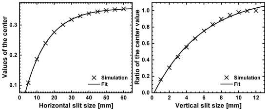
Figure A1. (left) Simulated normalized intensity for the Hgap experiment with $g_H=\mathrm{const}.=12$ mm and $d_{\mathrm{scat}}=6$ mm. The curve fits an exponential (Equation (7)) to the simulated data, yielding $d_{\mathrm{scat},\mathrm{H}}=6.792$ mm and $I_{\mathrm{scat},\mathrm{H}}=0.460$. (right) Ratio of simulated intensities from the rect experiment with respect to the same horizontal opening in Hgap based on $d_{\mathrm{scat}}=6$ mm. The curve fits an exponential (Equation (7)) to the simulated data yielding $d_{\mathrm{scat},\mathrm{V}}=2.68$ mm.

Appendix A.2

Estimating $h(x,y)$ from edge profiles, i.e., calculating MTF from LSF, does not reproduce $d_{\mathrm{scat}}$ correctly. Since $h_{\mathrm{scat}}(x,y)$ is not Gaussian, LSF is not a line profile across PSF but a convolution of the latter with Dirac’s delta distribution:

$$\begin{array}{c}\hfill \begin{array}{cc}\hfill \mathrm{LSF}\left(x\right)& =({\delta }_D\left(x\right)\ast h_{\mathrm{scat}}(x,y))\hfill \\ \hfill & ={\mathcal{F}}^{-1}\left[\mathcal{F}\left\{{\delta }_D\left(x\right)\right\}·\mathcal{F}\left\{h_{\mathrm{scat}}(x,y)\right\}\right]\hfill \\ \hfill & ={\mathcal{F}}^{-1}\left[{\delta }_D\left(u_y\right)·H_{\mathrm{scat}}(u_x,u_y)\right]\hfill \end{array}\end{array}$$

(A2)

Hence, in Fourier space, $\mathrm{MTF}\left(u_x\right)$ is indeed a line profile $H_{\mathrm{scat}}(u_x,0)$. However, since $H_{\mathrm{scat}}(u_x,u_y)$ is not available analytically (Hankel transform of $h_{\mathrm{scat}}\left(r\right)$ in Equation (A1), we calculate its Fourier transform numerically.

Figure A2 compares $\mathrm{MTF}\left(u_x\right)$ to a Lorentzian, i.e., the 1D Fourier transform of the exponential in Equation (1), as well as $\mathrm{LSF}\left(x\right)$ according to Equation (A2) to the same exponential. Fitting a Lorentzian to $\mathrm{MTF}\left(u_x\right)$ yields a good match for the peak and a moderate for the tails. However, the simulation shows that $d_{\mathrm{scat}}$ is overestimated by a factor of $1.385$ this way.

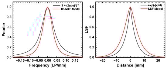
Figure A2. (left) Simulation of $\mathrm{MTF}\left(u_x\right)$ compared to Lorentzian (FT of 1D exponential). (right) Simulation of $\mathrm{LSF}\left(x\right)$ compared to 1D exponential (Equation (1)). Both assume $d_{\mathrm{scat}}=5$ mm.

References

- Riechert, F.; Bastian, G.; Lemmer, U. Laser speckle reduction via colloidal-dispersion-filled projection screens. Appl. Opt. 2009, 48, 3742–3749. [Google Scholar] [CrossRef] [PubMed]
- Li, Y.; Xu, Y.; Yang, Y.; Jia, Z.; Tang, H.; Patel, J.B.; Lin, Q. Template-Assisted Fabrication of Flexible Perovskite Scintillators for X-Ray Detection and Imaging. Adv. Opt. Mater. 2023, 11, 2300169. [Google Scholar] [CrossRef]
- Partridge, M.; Evans, P.M.; Symonds-Tayler, J.R.N. Optical scattering in camera-based electronic portal imaging. Phys. Med. Biol. 1999, 44, 2381–2396. [Google Scholar] [CrossRef] [PubMed]
- Siewerdsen, J.H.; Jaffray, D.A. Cone-beam computed tomography with a flat-panel imager: Magnitude and effects of X-ray scatter. Med. Phys. 2001, 28, 220–231. [Google Scholar] [CrossRef] [PubMed]
- Engel, K.J.; Herrmann, C.; Zeitler, G. X-ray scattering in single- and dual-source CT. Med. Phys. 2007, 35, 318–332. [Google Scholar] [CrossRef] [PubMed]
- Siewerdsen, J.H.; Moseley, D.J.; Bakhtiar, B.; Richard, S.; Jaffray, D.A. The influence of antiscatter grids on soft-tissue detectability in cone-beam computed tomography with flat-panel detectors: Antiscatter grids in cone-beam CT. Med. Phys. 2004, 31, 3506–3520. [Google Scholar] [CrossRef] [PubMed]
- Endo, M.; Tsunoo, T.; Nakamori, N.; Yoshida, K. Effect of scattered radiation on image noise in cone beam CT. Med. Phys. 2001, 28, 469–474. [Google Scholar] [CrossRef] [PubMed]
- Seibert, J.A.; Boone, J.M. X-ray scatter removal by deconvolution. Med. Phys. 1988, 15, 567–575. [Google Scholar] [CrossRef] [PubMed]
- Maltz, J.; Blanz, W.E.; Hristov, D.; Bani-Hashemi, A. Cone beam X-ray scatter removal via image frequency modulation and filtering. In Proceedings of the 2005 IEEE Engineering in Medicine and Biology 27th Annual Conference, Shanghai, China, 17–18 January 2005; pp. 1854–1857. [Google Scholar] [CrossRef]
- Siewerdsen, J.H.; Daly, M.J.; Bakhtiar, B.; Moseley, D.J.; Richard, S.; Keller, H.; Jaffray, D.A. A simple, direct method for X-ray scatter estimation and correction in digital radiography and cone-beam CT. Med. Phys. 2005, 33, 187–197. [Google Scholar] [CrossRef] [PubMed]
- Baker, S.; Brown, K.; Curtis, A.; Lutz, S.S.; Howe, R.; Malone, R.; Mitchell, S.; Danielson, J.; Haines, T.; Kwiatkowski, K. Scintillator efficiency study with MeV X-rays. In Proceedings of the Hard X-Ray, Gamma-Ray, and Neutron Detector Physics XVI, San Diego, CA, USA, 17–21 August 2014; Burger, A., Franks, L., James, R.B., Fiederle, M., Eds.; SPIE: Bellingham, WA, USA, 2014; Volume 9213, p. 92130H. [Google Scholar] [CrossRef]
- Thompson, A.C.; Attwood, D.T.; Howells, M.R.; Kortright, J.B.; Robinson, A.L.; Underwood, J.H.; Kim, K.J.; Kirz, J.; Lindau, I.; Pianetta, P.; et al. X-Ray Data Booklet; Lawrence Berkeley Laboratory, University of California: Berkeley, CA, USA, 2009. [Google Scholar]
- Vijayakumar, J.; Dejea, H.; Mirone, A.; Muzelle, C.; Meyer, J.; Jarnias, C.; Dollman, K.; Zabler, S.; Paolasini, L.; Bellier, A.; et al. Multiresolution Phase-Contrast Tomography on BM18, a New Beamline at the European Synchrotron Radiation Facility. Synchrotron Radiation News; Taylor & Francis: Abingdon, UK, 2024; pp. 1–10. [Google Scholar]
- Cianciosi, F.; Buisson, A.L.; Tafforeau, P.; Van Vaerenbergh, P. BM18, the New ESRF-EBS Beamline for Hierarchical Phase-Contrast Tomography. In Proceedings of the 11th Mechanical Engineering Design of Synchrotron Radiation Equipment and Instrumentation, MEDSI2020, Chicago, IL, USA, 24–29 July 2021. [Google Scholar] [CrossRef]
- Rakić, A.D.; Djurišić, A.B.; Elazar, J.M.; Majewski, M.L. Optical properties of metallic films for vertical-cavity optoelectronic devices. Appl. Opt. 1998, 37, 5271. [Google Scholar] [CrossRef] [PubMed]
- Polyanskiy, M.N. Refractiveindex.info database of optical constants. Sci. Data 2024, 11, 94. [Google Scholar] [CrossRef] [PubMed]
- Koch, A.; Raven, C.; Spanne, P.; Snigirev, A. X-ray imaging with submicrometer resolution employing transparent luminescent screens. J. Opt. Soc. Am. A 1998, 15, 1940. [Google Scholar] [CrossRef]
- Diez, M.; Saeidnezhad, N.; Tafforeau, P.; Zabler, S. Benefits of front coating crystalline scintillator screens for phase-contrast synchrotron micro-tomography. Opt. Express 2024, 32, 41790. [Google Scholar] [CrossRef] [PubMed]
- Michail, C.M.; Fountos, G.P.; Valais, I.G.; Kalyvas, N.I.; Liaparinos, P.F.; Kandarakis, I.S.; Panayiotakis, G.S. Evaluation of the Red Emitting Gd2O2S:Eu Powder Scintillator for Use in Indirect X-Ray Digital Mammography Detectors. IEEE Trans. Nucl. Sci. 2011, 58, 2503–2511. [Google Scholar] [CrossRef]
Disclaimer/Publisher’s Note: The statements, opinions and data contained in all publications are solely those of the individual author(s) and contributor(s) and not of MDPI and/or the editor(s). MDPI and/or the editor(s) disclaim responsibility for any injury to people or property resulting from any ideas, methods, instructions or products referred to in the content. |
© 2025 by the authors. Licensee MDPI, Basel, Switzerland. This article is an open access article distributed under the terms and conditions of the Creative Commons Attribution (CC BY) license (https://creativecommons.org/licenses/by/4.0/).