The Influence of Annealing Temperature on the Microstructure and Performance of Cold-Rolled High-Conductivity and High-Strength Steel

Abstract

Low-carbon micro-alloyed steel has become a wire material with great potential for further development due to its excellent comprehensive performance; however, there is still a lack of insight into the evolution of its electrical conductivity during annealing treatment after undergoing deformation. In this present contribution, we systematically explored the intrinsic correlation between the microstructural characteristics (including grain size evolution, dislocation density change, etc.) and performance indexes of cold-rolled high-conductivity high-strength steels and their mechanisms, using the annealing temperature, a key process parameter, as a variable. Characterization methods were used to comprehensively investigate the variation rule of the electrical conductivity of low-carbon micro-alloyed steels containing Ti-Nb elements under different annealing temperatures, as well as their influencing factors. The results show that for the ultra-low-carbon steel (0.002% C), the dislocation density continuously decreases with the increasing annealing temperature. Both experimental steels underwent complete recrystallization at 600 °C, with grain growth increasing at higher temperatures (with ultra-low-carbon steel being finer than low-carbon steel (0.075% C)). Dislocation density in ultra-low-carbon steel decreased steadily, whereas low-carbon steel exhibited an initial decline followed by an increase due to carbon-rich precipitate pinning. The yield ratio decreased with the annealing temperature, with optimal performance being at 700 °C for ultra-low-carbon steel (lowest resistivity: 13.75 μΩ/cm) and 800 °C for low-carbon steel (best conductivity: 14.66 μΩ/cm). Yield strength in ultra-low-carbon steel was dominated by grain and precipitation strengthening, while low-carbon steel relied more on precipitation and solid solution strengthening. Resistivity analysis confirmed that controlled precipitate size enhances conductivity.

1. Introduction

Grid transmission lines play a crucial role in the transmission, regulation, and configuration of electric energy in power grids. Among these, the wire is the main carrier of power transmission, which operates in a variety of geographical and climatic environments. Therefore, the wire material needs to possess excellent tensile strength and electrical conductivity. Microalloying technology, a significant advancement in the 20th-century steel industry, typically incorporates elements such as Nb, Mo, Ti, and V into lower-carbon steel to improve tensile strength and plasticity. Thus, low-carbon micro-alloyed steels are promising candidates for wire materials. To realize the unity of high strength and electrical conductivity in alloys, researchers have conducted in-depth studies on the microstructure and performance of alloys. Wang et al. [1] found that the addition of Fe and P could promote the precipitation of a large number of Cr and Cr₃P particles with even and finely dispersed features in the Cu-0.8Cr alloy. The progressive enhancement of precipitate particles is accompanied by an improvement in conductive properties, thereby optimizing the conductivity and tensile strength simultaneously. Wang Song et al. [2] studied the influences of the precipitation and growth processes of precipitated phases and the morphology of precipitated phases on the conductivity of Cu-4Ag-0.8Cr alloys. The conductivity of these alloys was significantly promoted through the precise tailoring of the micromorphology, the grain size, and the arrangement of alloy precipitates. Jiang et al. [3] prepared Al-Zr nanophases with a size of approximately 6 nm in Al-Zr alloys through a nanostructuring strategy, resulting in the highest degree of precipitation reinforcement, the smallest local strain field, and reduced scattering of electron motion, achieving the unification of high strength and high conductivity in alloys. In recent years, research on low-carbon micro-alloy steels has mainly focused on second-phase precipitation strengthening. Among them, Ti primarily scavenges nitrogen, inhibits grain growth, and improves weldability [4,5,6]. Nb exhibits a strong grain refinement effect in steel, and a small amount of Nb can significantly enhance steel toughness [7,8,9,10]. Ti-Nb composite microalloying is considered a significant means of satisfying the property requirements in steel. (Nb, Ti)(C, N) nanoparticles in steel hinder dislocation motion, serving as the primary strengthening mechanism [11,12,13]. Research has shown that the addition of micro-alloy components that contain Ti, Nb, and V may improve the grain structure of steel wires and enhance their strength ductility synergy. Nevertheless, there has been relatively little attention paid to the kind of steel wire [14,15], and there is a noted lack of systematic studies on the wire’s electrical properties [16]. Therefore, progress in the domain of high-strength and highly-conductive micro-alloyed steel can significantly benefit industries that require mechanical robustness and electrical efficiency, such as power transmission and automotive systems. This study also provides a theoretical reference for expanding the application scope of micro-alloyed steel.

This paper investigates the intrinsic relationship and variation mechanisms between the critical factor of annealing temperature and the microstructure (e.g., grain size, dislocation density) and performance of cold-rolled high-strength and high-conductivity steel in order to obtain a theoretical basis and practical reference point for optimizing steel performance to meet diverse engineering requirements. The annealing temperature serves as a critical parameter that modulates the material’s recrystallization kinetics while simultaneously governing its microstructural defect concentration. This dual influence exerts a significant influence on both electrical transport characteristics and mechanical integrity through microstructure evolution mechanisms. To identify the optimal annealing temperature for enhancing electrical conductivity and mechanical performance, this study examines the conductivity variations and influencing factors in micro-alloyed steel containing Ti and Nb with a low carbon content after annealing at various temperatures. It systematically analyzes the steel’s microstructure, mechanical behavior, and electrical conductivity while elucidating the impact mechanisms of precipitate morphology, size, and distribution with respect to material performance.

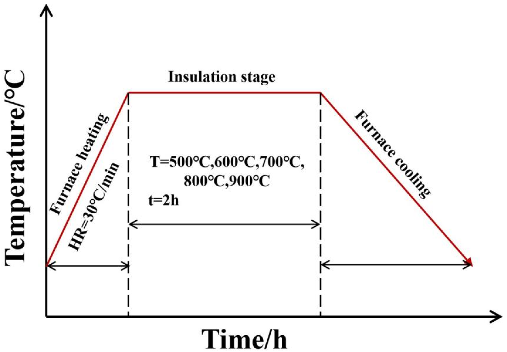
2. Experimental Materials and Methods

2.1. Experimental Material

This study used two micro-alloyed steels: ultra-low-carbon (1# steel) and low-carbon (2# steel). These were smelted in a laboratory vacuum induction furnace and cast into billets. The billets were then hot-rolled, pickled, and cold-rolled into plates. Their chemical compositions are shown in

Table 1. Component of experimental steel (wt.%).

	C	Si	Mn	P	S	Al	Nb	Ti	B	Fe
1#	0.0025	0.0120	0.3330	0.0294	0.0042	0.0452	0.0230	0.0393	0.0001	Bal.
2#	0.0579	0.0370	0.7130	0.0170	0.0039	0.0300	0.0159	0.0011	0.0003	Bal.

. Samples were taken from the cold-rolled steel plate along the rolling direction and annealed. The annealing heat treatment was conducted in a chamber electric furnace, with an annealing range of 500–900 °C, a gradient of 100 °C, and a holding time of 2 h, and the cooling method is furnace cooling. The specific annealing process is displayed in Figure 1.

2.2. Microstructure Characterization

Metallographic structure observation was conducted under a metallographic microscope. The observation surface was the rolled cross-section of the sample. After grinding the samples and polishing the ones, the steels suffered from corrosion with 4% alcohol nitrate solution and Marshall’s solution (A: 100 mL of distilled water, 8 g of oxalic acid, and 5 mL of sulfuric acid; B: 30% hydrogen peroxide solution; Liquid A was mixed with Liquid B in equal proportions). Subsequently, the microstructure changes of the rolled cross-section (RD-ND) were analyzed and characterized by FE-SEM with EBSD. The preparation of EBSD specimens is almost identical to that of the SEM specimens in terms of processing. The difference lies in the final step, where electrolytic polishing with a 10% perchloric acid–alcohol solution is required to remove surface stresses from the specimen. The EBSD results were obtained by the software of HKL Channel 5 (2019 v5.12), and the recrystallization volume fraction was obtained by analyzing the EBSD data through Channel 5 software. We calculate the grain orientation spread (GOS) value of each grain in Channel 5 and set the threshold value (GOS < 1° for recrystallized grains, GOS > 2° for deformed grains, and the middle is the restitution region), and the software statistically obtains the volume percentage of recrystallized grains. Finally, the dislocation distribution, composition, grain size, and arrangement of the precipitated nano-phase were explored and analyzed using TEM.

The phase composition and dislocation density of the samples were analyzed and calculated using X-ray diffraction. According to the report of Gay et al. [17], with the evolution of the half-height and width of the diffraction peak, the dislocation density ρ may be obtained via the Dunn formula [18]:

$$\rho ={\displaystyle \frac{{\beta }^2}{2\mathit{ln}2\pi b^2}}$$

(1)

where β is the half the width and height of the diffraction peak, the size of which can be analyzed by Jade software (pro 8.7); and b is the ferritic Berschner vector (0.248 nm).

2.3. Transmission Electron Microscopy Analysis

Microstructure observation and crystal structure analysis were performed using TEM with selected-area electron diffraction (SAED) and an energy-dispersive X-ray spectroscopy (EDX) detector. Samples were cut into 12 mm × 12 mm × 0.3 mm sheets, ground to a 0.06 mm thickness using 400–3000 grit metallographic sandpaper, and punched into Φ3 mm discs. The thin foils were prepared using electrolytic double-jet polishing in a 10% HClO₄ + 90% ethanol solution at 25 V DC and −20 °C (transmittance: 100%) for samples of TEM. Polished samples were washed with ethanol, air-dried, and placed in TEM holders.

2.4. Inductively Coupled Plasma Optical Emission Spectrometer (ICP-OES) Analysis

A powder sample with a medium mass of 1 g was taken from the test steel file using a file and added to a container containing an HCl + HNO₃ (aqua regia) dissolvent. The container was put in a water bath, heated to 70 °C, and held at a constant temperature for 6 h to ensure that the sample powder could be completely dissolved. When the dissolution process was finished, the solution could be filtered using a quantitative filter paper, and the solution was poured into a volumetric flask marked with L mL. After the filtration was completed, the container was rinsed with distilled water, the filter paper was rinsed with hydrochloric acid, and finally, the filter paper was rinsed one last time with distilled water. The solution in the volumetric flask was analyzed by an ICP-OES. The standard curve was obtained by configuring Ti and Nb standard solutions (1000 μg/mL) with concentration gradients of 0.01, 0.1, 1, and 10 μg/mL for the ICP test and linearly fitting the concentration points. Thereafter, by comparing with the standard curves of Ti and Nb with known concentrations, the concentrations of Ti and Nb in the solution were determined to be X µg/mL. We calculated the contents of solid-dissolved Ti and Nb in the sample according to the following formula:

$$w={\displaystyle \frac{X{L}_1}{M\times {10}^6}}\times 100\mathrm{\%}$$

(2)

2.5. Comprehensive Performance Test

Electrical resistivity was measured using a four-point probe tester on samples sized 12 mm × 12 mm × 1 mm. Each sample was measured five times, and the average value was taken. Meanwhile, the maximum and minimum values were excluded. Mechanical properties were evaluated via tensile testing on a universal testing machine (UTM) at a normal temperature. Tensile specimens (gauge length: 10 mm) were machined from heat-treated strips and tested at a crosshead speed of 0.01 mm/s. Three parallel tests were conducted per group, and the results were averaged.

3. Results

3.1. Microstructure Analysis

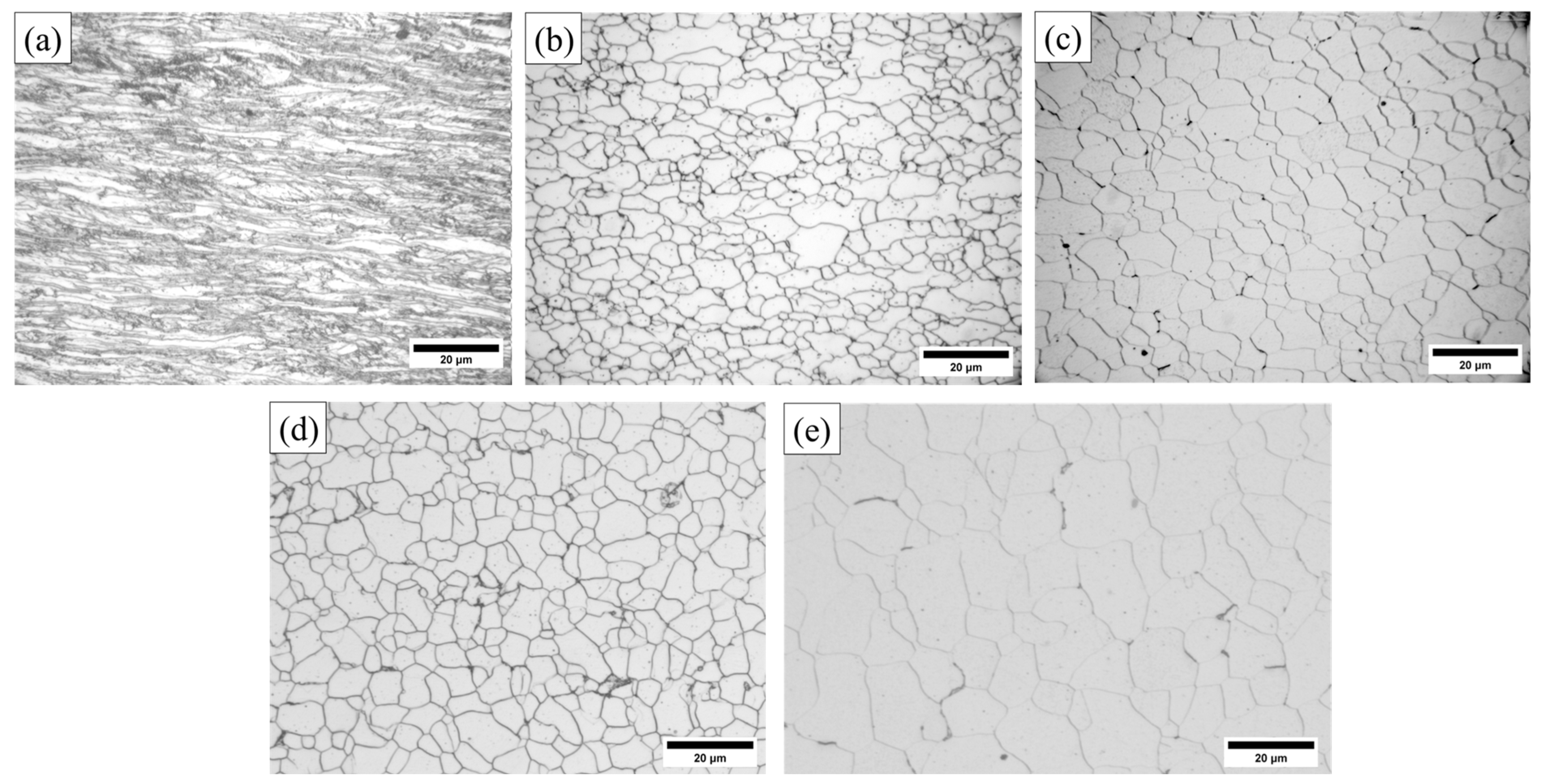
3.1.1. Metallographic Structure

Figure 2 shows the microstructural structure evolution of 1# steel after 2 h of isothermal annealing at various temperatures. As the annealing temperature rises from 500 °C, the initially elongated ferrite grains along the rolling direction gradually undergo homogenization, accompanied by distinct grain boundary formation and significant grain growth. This microstructural transformation stems from enhanced grain boundary mobility [19,20], where the grain growth rate directly correlates with boundary mobility. Consequently, elevated annealing temperatures promote grain boundary migration, leading to accelerated grain growth and ultimately resulting in coarser grains under a fixed annealing duration.

Figure 3 illustrates the microstructural evolution of experimental steel 2# following 2 h annealing at various temperatures. The microstructural transformation demonstrates a distinct temperature dependency, wherein the grain size gradually increases at elevated annealing temperatures. At 600 °C, the initially fragmented grains transitioned to equiaxed morphology, indicating complete recrystallization at this temperature.

Comparative analysis of the recrystallization behavior reveals that under identical annealing conditions, steel 2# exhibits significantly finer grains than 1# steel. This grain refinement effect stems from the higher percentage of carbon for 2# steel, which promotes the presence of microalloying carbon precipitates that effectively inhibit grain growth.

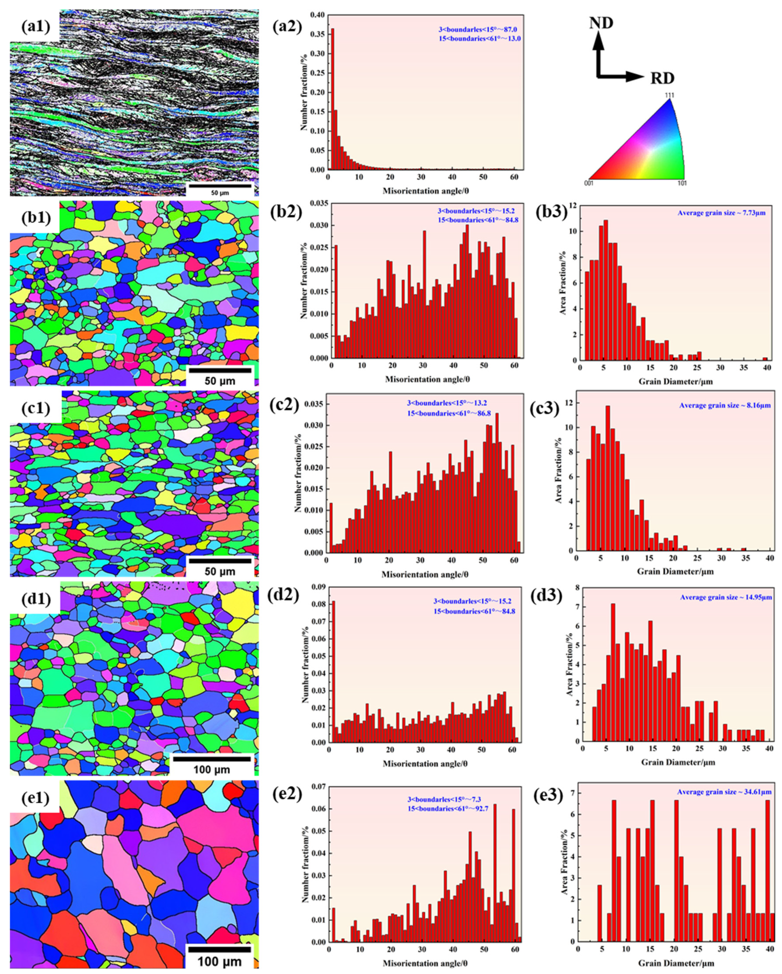
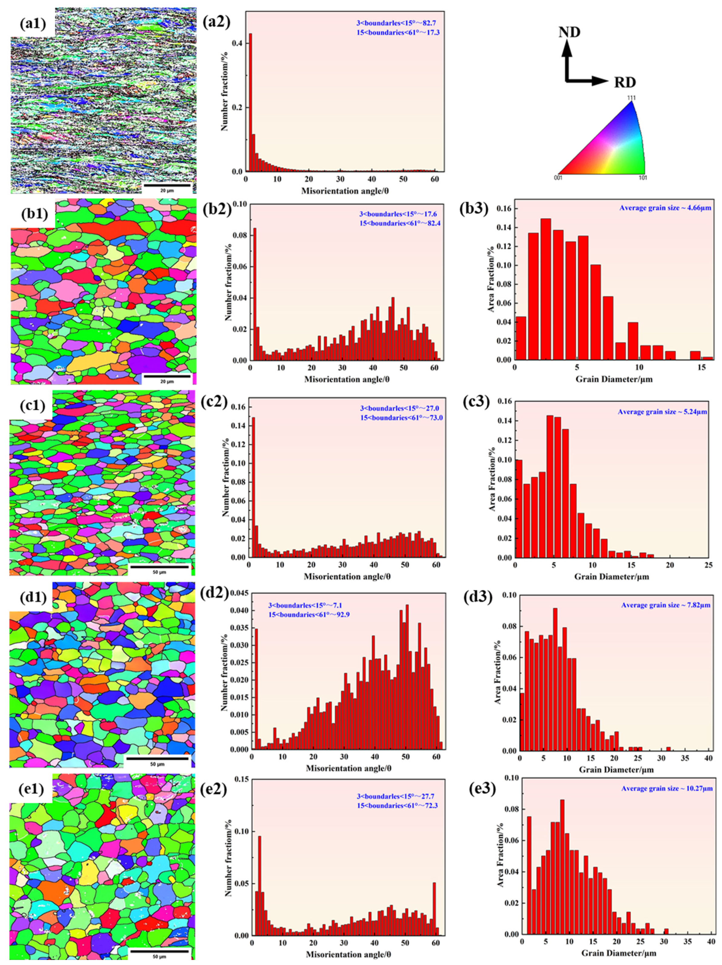
3.1.2. EBSD Analysis

Figure 4 exhibits the corresponding inverse pole figure (IPF) for the grain orientation difference and grain size distribution for 1# steel during recrystallization. In the IPF diagram, different colors express different grain orientations, in which the blue, red, and green parts indicate <111>//ND, <001>//ND, and <101>//ND directions, respectively. Black and white represent high-angle grain boundaries (HAGB) and low-angle grain boundaries (LAGB), respectively. It can be observed that with the increase in annealing temperature, the ratio of the <111>//ND and <001>//ND directions in 1# steel gradually increases, among which <111>//ND increases more. When the annealing temperature is 500 °C, the fibrous grain of 1# steel appears, and the density of the LAGB in the sample is higher (about 87.0%). These details indicate that the recrystallization process has not yet begun. When the annealing temperature rises, the average grain size increases, and the density of HAGB increases gradually. When the annealing temperature is 600 °C, the density of HAGB comes to 84.8%, and the deformed grains become equiaxed. In this case, the grain distribution is mostly small-diameter grains with an average size of 7.73 μm, which indicates that the recrystallization of the experimental steel has been completed. After that, the grain grows continuously with a continuously increasing annealing temperature, and the small-size grains grow faster than the large-size grains. Therefore, with the increase in the annealing temperature, although the grain is growing, the growth rate is gradually flattening. When the annealing temperature comes to 900 °C, the average grain size reaches 34.61 μm for 1# steel, and the grain distribution at this time is formed of mostly large-diameter grains.

The corresponding IPF and grain orientation difference in the recrystallization process of 2# steel are indicated in Figure 5. It can be seen that the proportions of the <111>//ND and <101>//ND orientations in 2# steel gradually increase with the increase in the annealing temperature, and the <101>//ND increases more. As with 1# steel, 2# steel has polygonal grains at 600 °C, the proportion of HAGB is about 82.4%, and grain recrystallization occurs. An average grain size of 4.66 μm is obtained. The ferrite grains grow gradually, accompanied by a gradual increase in annealing temperature. This is because the nucleation and grain growth rate increase when the annealing temperature increases, and the activation energy required for grain boundary movement decreases. When the annealing temperature is high, the recrystallization process will be completed in a short holding period; then, with the lengthening of holding time, the grains will continue to grow. Therefore, when the holding time is fixed, the higher the annealing temperature is, the coarser the grain becomes.

Table 2. Recrystallization fraction of both steel samples at various annealing temperatures.

	1#-500 °C	1#-600	1#-700	1#-800	1#-900	2#-500	2#-600	2#-700	2#-800	2#-900
Recrystallized	4.2	98.2	99.2	89.6	96.1	16.1	95.1	87.1	66.4	73.7
In transit	0.6	1.7	0.7	10.1	3.9	8.1	4.6	11.9	33.5	24.6
Uncrystallized	95.1	0.06	0.02	0.2	0.006	75.8	0.3	1.0	0.1	1.7

presents the recrystallization fractions of both steel samples under various temperature conditions. The recrystallization fraction of 1# steel does not vary considerably with an increase in the annealing temperature; instead, only the grain growth process varies. However, the recrystallization fraction of 2# steel changes dramatically when the annealing temperature is above 700 °C, showing a trend of decreasing and then increasing again. As the annealing temperature rises, a notable increase in grain size is observed, indicating that secondary recrystallization occurs at this time. This is due to the fact that the content of C in 2# steel is higher than that in 1# steel, and the microalloying elements Ti and Nb combine with C to form a second phase, which obstructs grain growth. Therefore, the grains finish recrystallizing at 600 °C, although they still contain smaller grains. As the annealing temperature rises, the smaller grains are absorbed by the larger grains, and the recrystallization fraction shows a trend of decreasing and then increasing.

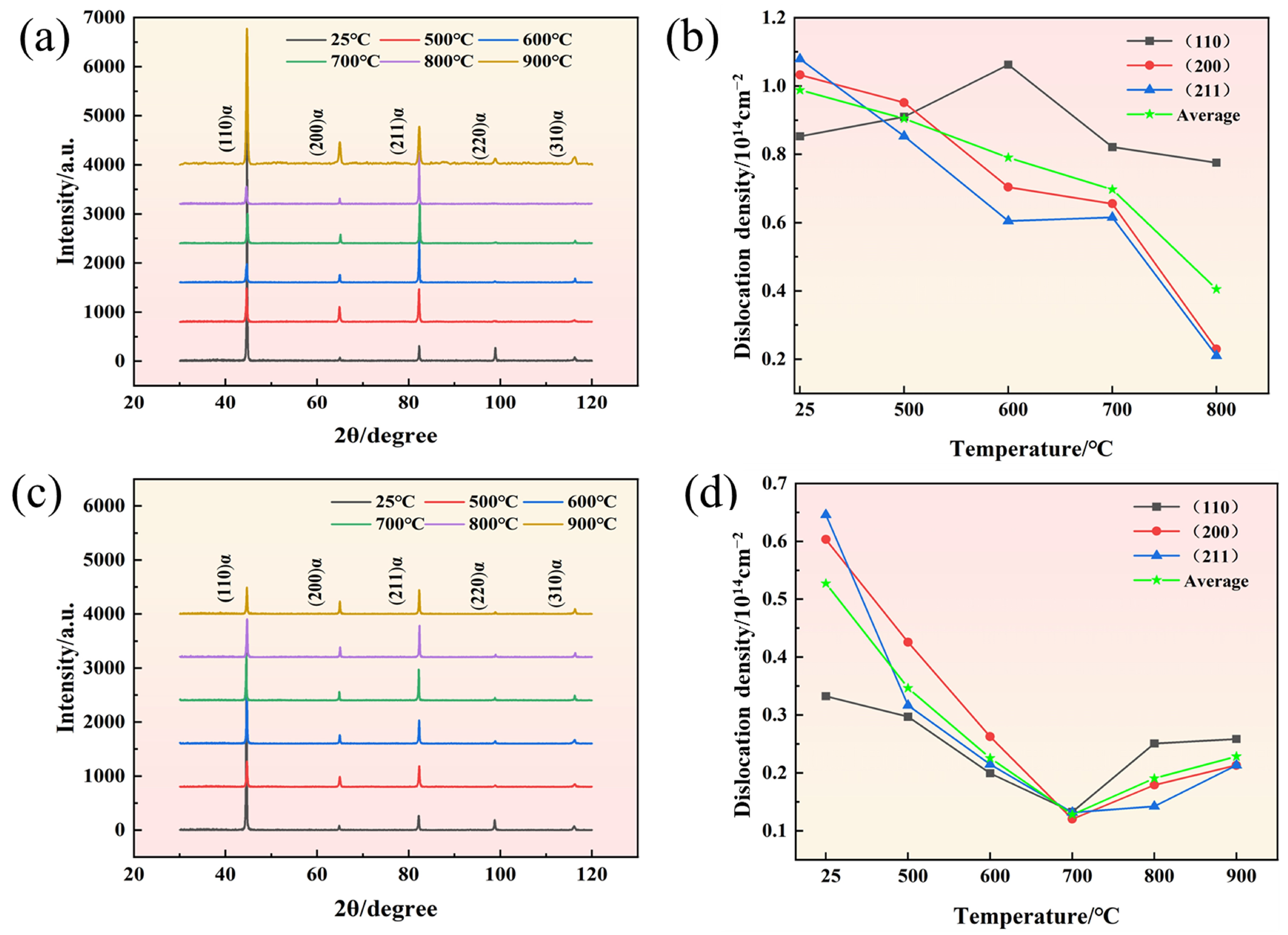
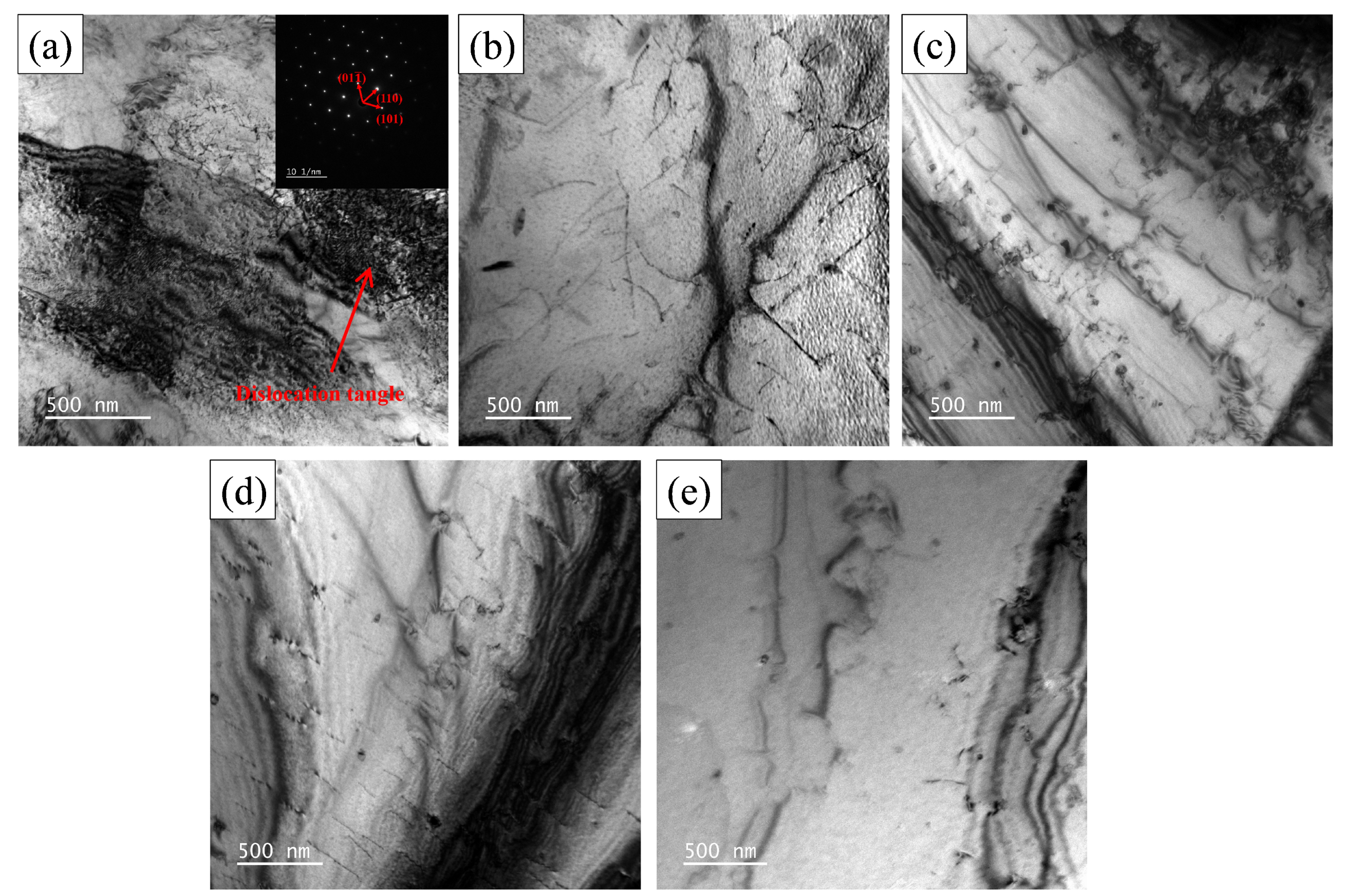
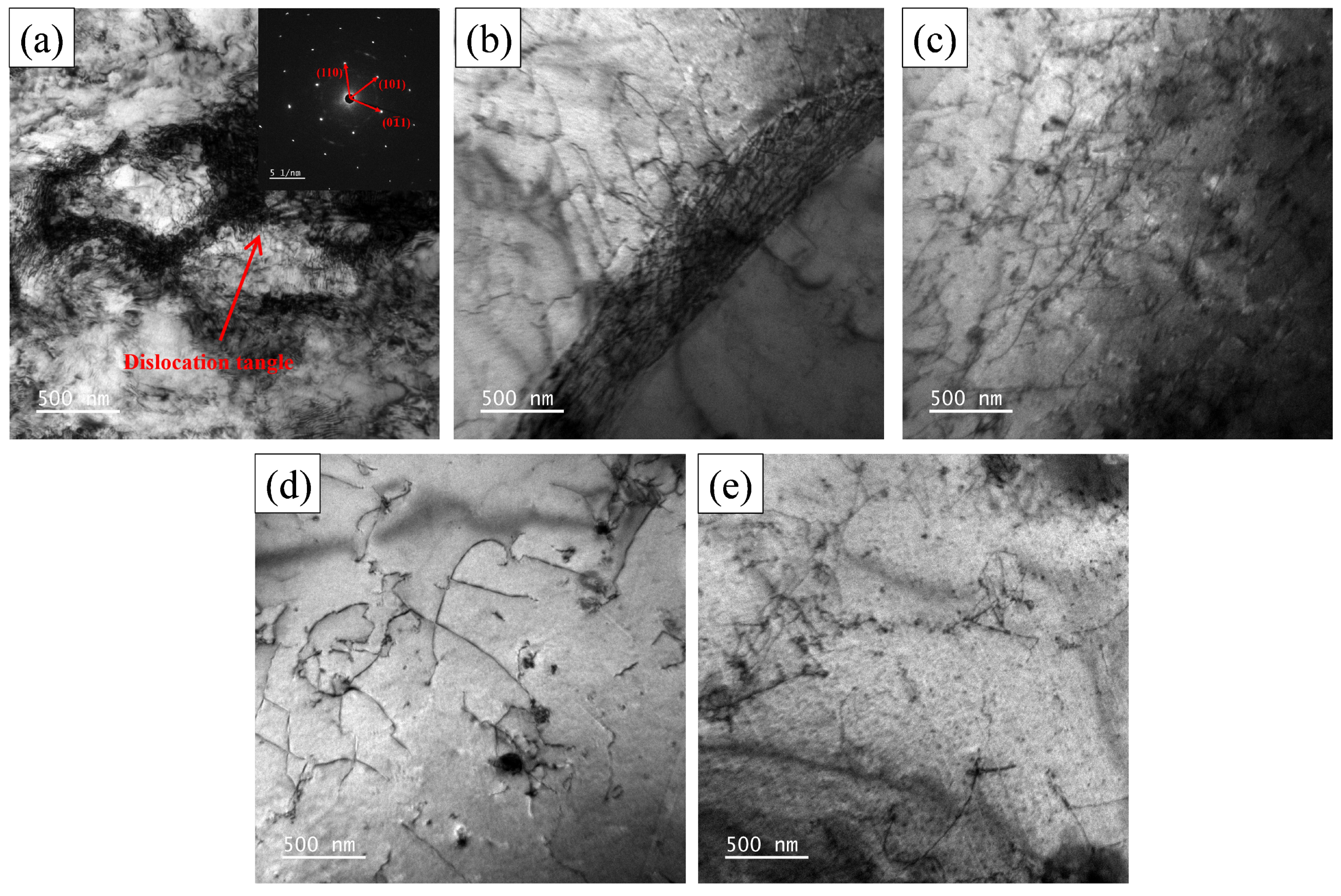
3.1.3. Dislocation Analysis

Figure 6a,b show the XRD pattern and the calculation results for the internal dislocation density of 1# steel after annealing at various temperatures. More obvious (110), (200), and (211) ferritic peaks were detected in 1# steel. The average internal dislocation density of 1# steel exhibited a declining trend as the annealing temperature increased. Higher annealing temperatures resulted in reduced internal dislocation density. Figure 6c,d show the XRD pattern and the calculation results of the internal dislocation density of 2# steel subjected to various heat treatment processes. At various annealing temperatures, 2# steel contains ferrite without the formation of new phases. The average internal dislocation of 2# steel exhibits a trend of initially decreasing and then subsequently increasing as the annealing temperature rises. At high annealing temperature, 2# steel contains more C, and the nanoscale precipitated phase is continuously precipitated, which has a cold-rolling effect on the dislocation and hinders the movement of the dislocation. The precipitated phase first precipitates at grain boundaries and then defects at lower temperatures. The first precipitated particles grow continuously, and the precipitated phase at the grain boundary causes lattice distortion in the grain and then produces new dislocation. The combination of the aforementioned factors leads to an increase in the dislocation density of 2# steel.

Figure 7 illustrates the temperature-dependent microstructural evolution of 1# steel as revealed by transmission electron microscopy (TEM). At 500 °C, the microstructure exhibits pronounced cellular dislocation networks with abundant low-angle grain boundaries (LAGBs), indicating residual stress retention and the predominance of recovery-dominated deformation mechanisms. The dislocation in the microstructure of 1# steel disappears significantly when the annealing temperature is 600 °C, indicating that there are new recrystallized grains in the microstructure and that the sample is in the recrystallization stage. Above 600 °C, with the increase in annealing temperature, the dislocation density in the 1# steel structure decreases significantly, and the dislocations are distributed in the grains in the shape of broken lines.

Figure 8 shows the TEM morphologies of 2# steel under various annealing temperatures. It can be observed that in the range of certain annealing temperatures, the dislocation density in the experimental steel structure drops with the increase in annealing temperature. When the annealing temperature is below 700 °C, the subgrain boundaries (the dislocation tangle shown by the red arrow in Figure 8a) and dislocation walls (Figure 8b) caused by dislocation entanglement can be observed. However, at an annealing temperature of 700 °C, the dislocation density decreases significantly, but there are still some dislocations that are pinned by the precipitated phase and remain.

In summary, the difference in the variation trend of dislocation density in 1# steel and 2# steel can be ascribed to the number of internal precipitates in the steel. When the annealing temperature increases, the internal dislocation density of the two steels decreases continuously. However, the content of C in 2# steel is high, the carbide precipitates grow continuously, and the number of precipitates increases at higher annealing temperatures. This, in turn, obstructs the movement of the dislocation and promotes the dislocation density.

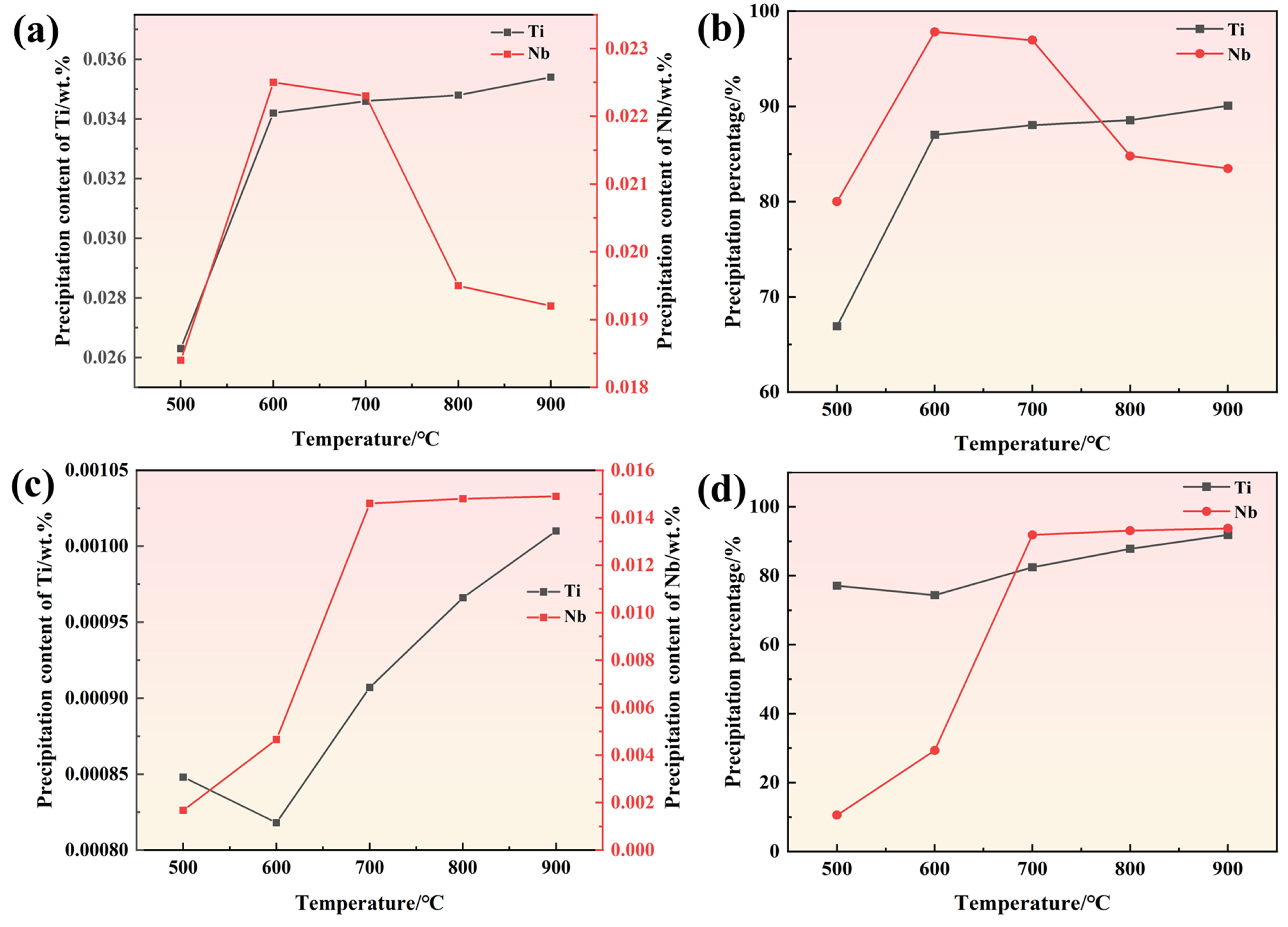
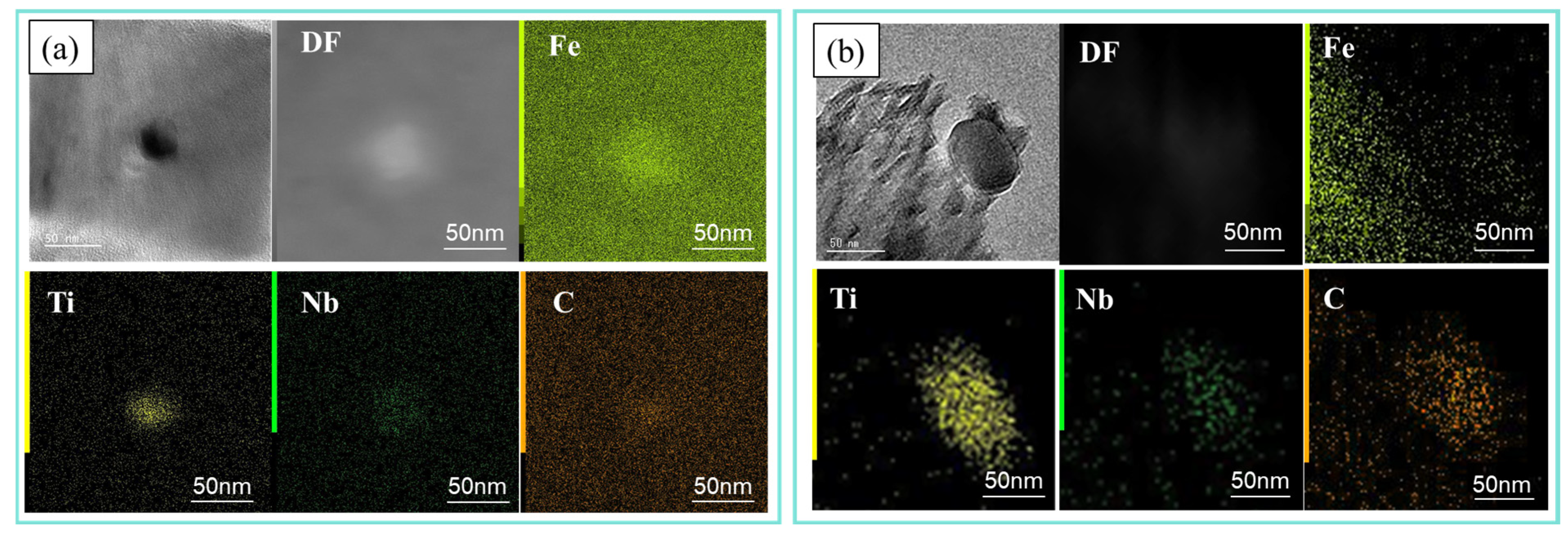
3.1.4. Precipitation Analysis

Figure 9 exhibits the distribution of precipitated phases of 1# steel held for 2h at various annealing temperatures. When the annealing temperature is 500 °C, a large number of dislocation entanglements exist, and no obvious precipitated particles are found. When the annealing temperature is 600 °C, the precipitated particles are found near the dislocation, and the size of the precipitated phase is small, which has a nail-rolling effect on the dislocation and further strengthens the steel. However, the decrease in dislocation density results in a decrease in the overall strength of the experimental steel. With the further increase in annealing temperature, the number of smaller precipitated phases increases, which results in a decrease in the resistivity of the experimental steel. However, when the annealing temperature is high, the size further increases, and the quantity gradually decreases for the precipitated phase.

The analysis of the composition of the precipitate phase was carried out using ICP technology. Figure 10 show the precipitates from 1# and 2# steel after 2 h of annealing at different temperatures. It can be observed that the precipitated mass fraction of Ti is generally larger than that of Nb because the Ti component in 1# steel is larger than that of Nb. With the increase in the annealing temperature, the precipitated mass fraction of Ti shows an increasing trend and eventually tends towards a stable value, but the precipitated mass fraction of Nb exhibits a trend of increasing initially and then decreasing. When the annealing temperature is low, the relative precipitation content of Nb is high, and the relative precipitation content reaches more than 95% with the increase in the annealing temperature within a certain temperature range. However, when the annealing temperature is high, the relative precipitation content of the Nb element shows a downtrend, and the relative precipitation content of the Ti element can reach 90%. According to ref. [21], in terms of thermal stability, the Ti in carbides is higher than Nb, and its resolution temperature is also higher. Therefore, it can be inferred that at a higher annealing temperature, the Nb in the precipitated phase will be solid-dissolved into the matrix again. Figure 10c,d show the mass fraction curve and relative percentage curve of Ti and Nb precipitated from 2# steel after annealing for 2 h at various temperatures. It can be observed that with the increase in annealing temperature, the precipitated mass fraction of Nb shows an increasing trend and eventually tends to a stable value, but the precipitated mass fraction of Ti shows an increasing trend in general. On account of the low content of Ti, the precipitation amount accounts for 80% of the total content when the annealing temperature is low. Meanwhile, the relative precipitation content of Nb is low, but with the increase in the annealing temperature, the relative precipitation content continues to increase. Within a certain temperature range, the relative precipitation content reaches more than 95% with the increase in annealing temperature. The higher the carbon content, the more carbon can participate in the formation of precipitates under the same conditions, providing more favorable conditions for the formation of precipitates. However, the mass fraction of the precipitate formed in 1# steel is higher than that in 1# steel (with a higher carbon content). This is because the relatively high content of Ti and Nb in the original sample is present, as shown in Table 1.

Figure 11 exhibits the distribution of the precipitated phase of 2# steel held for 2h at various annealing temperatures. At 500 °C, there are a large number of dislocation entanglements inside the 2# steel sample. When the annealing temperature is 600 °C, precipitated particles are found near the dislocation. With the increase in annealing temperature, the size of the precipitated phase increases further; however, the precipitated phase experiences a rapid increase in size at 900 °C.

Figure 12a shows the STEM-EDS spectrum of the precipitated phase of 1# steel annealed at 900 °C. It can clearly be observed that there is an enrichment of Ti, Nb, and C in the precipitated phase, and it can be inferred that the precipitated phase of the experimental sample is (Ti,Nb) C phase. Figure 12b shows the STEM-EDS spectrum of the precipitated phase of 2# steel at 900 °C. It can clearly be observed that there is an enrichment of Ti, Nb and C in the precipitated phase, and the precipitated phase is the same as that of 1# steel, which is (Ti,Nb) C phase. The DF in Figure 12 refers to the dark field image. The precipitates inside the two experimental steels are (Ti, Nb) C phases. Generally, a higher carbon content offers more carbon resources for precipitate formation under identical circumstances, thus creating more conducive conditions for the generation of precipitates. For example, in Ti/Nb micro-alloyed steel, the increase in carbon content leads to an uptrend in the number of precipitates (Ti/NbC). When the Ti/Nb content remains the same, based on theoretical analysis, the mass fraction of precipitates in 2# steel (characterized by a higher carbon content) should surpass that of precipitates in 1# steel. Nevertheless, the significantly higher Ti content in 1# steel actually displays a decisive effect in the precipitation process, over-riding the influence of carbon content on precipitate formation.

3.2. Comprehensive Performance

3.2.1. Mechanical Property

Figure 13 indicates the stress–strain relationship and mechanical properties of two experimental steels at various annealing temperatures. When the annealing temperatures were 600 °C and above, a significant yield plateau was observed in 1# steel. The cold-rolled samples before and after annealing at 500 °C did not show an obvious yielding plateau, and both showed continuous yield elongation. This can be attributed to the fact that the carbon component in 1# steel is very low, and after adding a certain amount of microalloying elements, the carbon atoms are fixed as carbides, thus eliminating the interaction between the gap atoms and the dislocation, so the uniaxial tensile properties exhibit continuous yielding characteristics. The yield and tensile strength of 1# steel continue to drop with the increase in the annealing temperature, and the yield strength ratio also shows a decreasing trend. The yield and tensile strength of the 1# steel cold-rolled sample decreased rapidly when the annealing temperature changed from 500 °C to 600 °C. Above 600 °C, the yield strength and tensile strength dropped slowly with the increase in annealing temperature. However, when the temperature was 900 °C, the yield strength was higher than that at 800 °C, and the yield ratio increased suddenly. In conjunction with Figure 11, it can be deduced that an overall increase in the strength of the experimental steels is obtained when the Nb is dissolved alone in the matrix at 900 °C. The elongation of 1# and 2# steel exhibits an initial increase followed by a decrease with the increase in annealing temperature. When the annealing temperature is under 700 °C, the gradual release of residual stresses and the significant reduction in dislocation density within the material, accompanied by pronounced recovery and recrystallization processes, lead to a remarkable improvement in plasticity and a continuous increase in elongation. However, when the annealing temperature reaches the 700–900 °C range, excessive temperature causes noticeable grain coarsening, and this microstructural degradation ultimately results in decreased elongation.

However, as shown in Figure 13b, there exists a clear yield stage in the stress–strain curve of the annealed state of 2# steel. This may be related to the dislocation motion [22]. In alpha Fe, the carbon atoms formed a Cauchy air mass (Cottrell atmosphere), pinning dislocation through their interaction with the dislocation, resulting in a higher yield after the dislocation motion was blocked. When the dislocation removes the pinning of the Cauchy air mass, it forms a lower yield after moving under low stress [23,24]. Simultaneously, the yield and tensile strength of 2# steel continue to drop with the increase in annealing temperature, while the yield strength ratio shows a decreasing trend.

During annealing, the steel undergoes recovery and recrystallization, effectively eliminating work hardening. This is accompanied by a significant reduction in dislocation density, primarily due to the partial annihilation of the initially entangled dislocation network. As a result, the barriers to the dislocation motion are weakened, leading to reduced strength and enhanced plasticity [25,26]. It is clear that a lower annealing temperature corresponds to a smaller grain size and, consequently, a higher tensile strength. The 2# steel sample has a smaller grain size and a higher tensile strength. Grain boundaries significantly hinder dislocation movement. Reducing grain size increases grain boundary density, strengthening dislocation pinning effects and overall deformation resistance.

3.2.2. Conductivity

Figure 14 shows the electrical resistivity and strength–resistance ratio of experimental steels with various annealing temperatures. The electrical resistivity of both experimental steels first decreases and then increases with the higher annealing temperature. The electrical resistivity of 1# steel is the lowest at an annealing temperature of 700 °C, while that of 2# steel is the lowest at an annealing temperature of 800 °C, indicating that the steel has the best conductivity. The strength–resistance ratio of both steels shows a decreasing trend with the increase in the annealing temperature. The difference in the strength-to-resistance ratio between the experimental steel annealed at 700 °C and 800 °C is not significant, but the difference in resistivity is significant. Therefore, the comprehensive performance of 1# steel is the best when annealed at 700 °C, but the comprehensive performance of 2# steel is the best when annealed at 800 °C. The fundamental reason for metal resistance is that the lattice scatters the movement of electrons, and the test steel conductivity is affected by the scattering of impurities caused by various defects that are caused, in turn, by the thermal vibration of atoms in the crystal [27]. Therefore, the more serious the lattice distortion within the tissue, the stronger the scattering of electrons, and the lower the conductivity of the test steel. However, in the case of increasing grain size, the resistivity does not continuously decrease, which indicates that the grain size is not the primary factor affecting conductivity in this experiment.

3.2.3. Phase Transition

Extensive investigations have been conducted into the phase transformations and their effects on the recrystallization and dislocation evolution of cold-rolled high-conductivity and high-strength steel containing Ti-Nb, with the annealing temperatures ranging from 500 °C to 900 °C [28]. At 500 °C, the nucleation and growth of nanoscale (Nb, Ti) (C, N) precipitation phases mainly occur in the Ti-Nb micro-alloyed steel. These precipitation phases pinned dislocations through the Orowan mechanism, but the dislocation density still shows a decreasing trend [29]. Recrystallization is almost completely inhibited at this stage, and the precipitation phases impede the migration of HAGB through the Zener pinning effect. At 600 °C, the grain size for the precipitation phases increases, leading to discontinuous characteristics in the kinetics of recrystallization. The dislocation network begins to decompose into movable dislocation segments, but the chemical interaction between the precipitation phases and dislocations (such as the Suzuki effect) still dominates the hardening behavior [30]. At 700 °C, the recrystallization process accelerates, with a completion degree of >90%. The grain size distribution tends to be uniform. Residual precipitation phases are enriched at the austenite/ferrite phase boundaries, leading to the hindrance of local grain growth and the formation of a bimodal grain structure [31]. At 800 °C, the temperature exceeds the dissolution critical point of the precipitation phases, and NbC begins to dissolve. The volume ratio of the precipitation phases drops below 0.1%. At 900 °C, the phase change from ferrite to austenite results in an increase in grain boundary mobility by 2–3 orders of magnitude, and the dislocation density drops below 10% of that in the initial cold-rolled state [32]. The TiN particles are completely dissolved; the tendency towards abnormal grain growth is significant [33].

4. Discussion

4.1. Strengthening Mechanism

We estimated the individual effect of each reinforcement mechanism using various methods described in the literature. The enhancing contribution of experimental steel can be calculated using Equation (3) [34,35,36]:

$${\sigma }_y={\sigma }_0+{\sigma }_{ss}+{\sigma }_g+{\sigma }_{\rho }+{\sigma }_p$$

(3)

where σ₀ indicates lattice strengthening; (the value of σ₀ in this article is 48 MPa [37]); σ_ss indicates solid solution strengthening; σ_g indicates fine crystal strengthening; σ_ρ indicates dislocation strengthening; and σ_p indicates precipitation strengthening. Their units are all in MPa.

Solution strengthening is estimated by the following formula [38,39]:

$${\sigma }_{ss}=37\left[Mn\right]+83\left[Si\right]+470\left[P\right]+4570\left[C\right]+3750\left[N\right]$$

(4)

where [M] (M = C, N, Mn, etc.) represents the mass percentage of elements in the ferrite [39]. Silicon, manganese, and phosphorus atoms are generally considered to be completely solid-soluble. Steel does not contain nitrogen, and the value of [N] is considered to be 0. The component of [C] in 1# steel is low, and it is considered that the [C] element is completely precipitated.

The grain size and substructure characteristics, as intrinsic strengthening elements of metallic materials, have a significant regulatory effect on their mechanical properties. At present, the Hall–Petch relationship is still the main theoretical model for quantitatively characterizing the strengthening effect, and its incremental strength (σ_g) can be predicted by establishing a quantitative analysis model. The specific mathematical expression is as follows [39,40]:

$${\sigma }_g=k{d^{-}}^{{\displaystyle \frac{1}{2}}}$$

(5)

where k denotes the Hall–Petch coefficient (MPa m^1/2); d represents the mean ferritic grain size (m); and for high-strength micro-alloyed steels, the k value is experimentally determined as 0.55 MPa·m^1/2 [39].

The dislocation density inside the specimen gradually increases in the course of cold rolling, causing an increase in the yield strength (σ_y), which can be obtained using the Taylor equation [39,41,42]:

$${\sigma }_{\rho }=\alpha MGb{\rho }^{{\displaystyle \frac{1}{2}}}$$

(6)

where α denotes the geometric constant (α ≈ 0.38); M represents the Taylor factor for dislocation glide (M = 2.2 in body-centered cubic ferritic grains); G corresponds to the shear modulus (G = 81.6 GPa characteristic of low-carbon steels); b indicates the magnitude of the Burgers vector (b = 2.5 × 10⁻¹⁰ m, as defined by the steel’s crystal structure); and ρ specifies the spatial distribution density of mobile dislocations within the microstructure [39,42].

In order to quantitatively and deeply understand the influence of precipitation enhancement, it is generally believed that the role of the precipitated phases is achieved via the bypass method with respect to particles with unchanged shapes. In terms of Gladman’s way, the Ashby–Orowan modified model is adopted, and precipitation strengthening is expressed via the following equation [43]:

$${ \sigma }_p={\displaystyle \frac{5.9\sqrt{f}}{r}}ln\left({\displaystyle \frac{r}{2.5\times {10}^{-4}}}\right)$$

(7)

where r indicates the radius (μm) of the emerging particle; and f is the volume ratio of the particle, derived from Archimedes’ formula for density, volume, and mass:

$$f={\displaystyle \frac{f_m\times {\rho }_{Fe}}{{\rho }_p}}$$

(8)

where f_m is the mass percentage of emerging particles, which may be analyzed and obtained via physical and chemical technology; and ρ_p is the density of the precipitated phase [38].

Figure 15 presents a comparative analysis between the experimental yield strength and the theoretical yield strength for the two steel samples. The yield strength of 2# steel is generally higher than that of 1# steel, which is associated with the C content presence in the experimental steel. Due to the coarse grain size of 1# steel following annealing at 900 °C, its grain strengthening calculation formula becomes inapplicable, leading to a substantial discrepancy between the calculated and experimental values. Without considering the intrinsic enhancement, the yield strength of the 1# sample is mainly contributed by fine grain and precipitation enhancing, and the yield strength of the 2# sample is briefly derived from precipitation and solution enhancing. Therefore, it can be concluded that the precipitated phases may promote the strength of the samples to a certain extent.

4.2. Influence Mechanism of Conductivity

The total resistivity of materials can be expressed according to Mattiessen’s rule as follows [18,44]:

$${\rho }_{total}={\rho }_0+{\rho }_{ss}+{\rho }_d+{\rho }_{GB}+{\rho }_p$$

(9)

where ρ_total represents the total resistivity of the sample; ρ₀ represents the inherent resistivity of original sample, which, in this experiment, is 9.78 μΩ·cm [39]; and ρ_ss, ρ_d, ρ_GB, and ρ_p denote the resistivities due to solute atoms, dislocations, grain boundaries, and precipitates, respectively.

In the various influencing parameters, grain boundaries and solute atoms have a significant impact on the conductivity of the test sample, while the influence of dislocations and precipitated phases is relatively weak. In particular, the scattering behavior of solute atoms displays a crucial effect in determining the whole electrical resistivity of the sample [45]. Based on this, it can be inferred that the annealing temperatures exceeds 700 °C. As the solute atomic content increases, the electrical resistivity of the test sample will increase, which will significantly affect its conductivity.

When the grain is treated as equiaxed, the resistivity (ρ_GB) caused by grain boundaries may be calculated by Equation (10) [46]:

$${\rho }_{GB}=3{\displaystyle \frac{{\rho }_{GB}^0}{d}}$$

(10)

where ${\rho }_{GB}^0$ represents the resistivity for the unit area density at the grain boundary in the equilibrium state, and d shows the grain size.

The dislocation-induced resistivity (ρ_d) can be calculated by Equation (11) [47]:

$${\rho }_{\mathrm{d}}=K_{SD}\times \lambda$$

(11)

where K_SD is the specific dislocation resistivity and λ indicates the dislocation density. The dislocation-induced resistivity is directly proportional to the dislocation density.

The resistivity (ρ_ss) due to the solution can be calculated by the following formula [22]:

$${\rho }_{ss}=X\times \Delta \rho$$

(12)

where X (at. %) expresses the percentage of solute atoms, and Δρ represents the rising value of the sample’s resistivity when the number of solid-solution atoms increases by 1 at.%.

Since there is no interaction between the precipitated phases, the approximate expression of the alloy conductivity can be established based on the conductivity and volume percentage of the precipitates dispersed on the alloy matrix according to the Schroder formula [22]:

$${\rho }_p={\rho }_{total}-{\rho }_m$$

(13)

$${\displaystyle \frac{1}{{\rho }_{total}}}={\displaystyle \frac{1}{{\rho }_m}}\left(1-{\displaystyle \frac{2}{3}}f\right)$$

(14)

where f denotes the volume percentage of precipitates, and ρ_m denotes the resistivity of the inner steel, including grain boundaries, dislocations, solute atoms, and other factors.

The resistivity, known grain size, dislocation density, and solid solution atom content obtained by the experiment are put into the following formula:

$$\begin{array}{cc}{\rho }_{total}& ={\rho }_0+3{\displaystyle \frac{{\rho }_{GB}^0}{d}}+K_{SD}\times \lambda +X\times \Delta \rho +{\displaystyle \frac{2f}{3-2f}}{\rho }_m\\ & =9.78+{\displaystyle \frac{3A}{d}}+B\times \lambda +X\times C\\ & +{\displaystyle \frac{2f}{3-2f}}\left({\displaystyle \frac{3A}{d}}+B\times \lambda +X\times C\right)\\ & =9.78+{\displaystyle \frac{3}{3-2f}}({\displaystyle \frac{3A}{d}}+B\times \lambda +X\times C)\end{array}$$

(15)

By inserting the known data of the experimental steel into the above equation, we obtain A = 8.126, B = 0.542, C = 91.482; then, the above equation can be converted to the following:

$${\rho }_{total}=9.78+{\displaystyle \frac{3}{3-2f}}\left({\displaystyle \frac{24.378}{d}}+0.524\lambda +91.482X\right)$$

(16)

We substituted all the data into the formula for verification and obtained the resistivity data given in

Table 3. Resistivity calculation and test values.

	1-600	1-700	1-800	1-900	2-600	2-700	2-800	2-900
Test value	13.99	13.75	15.02	13.77	15.16	15.14	14.66	15.40
Calculated value	13.99	13.74	12.25	10.99	15.89	14.76	13.19	12.43
Error	0	0	18%	20.18%	4.8%	2.5%	10%	19%

. The formula obtained has a large degree of error in calculating large particle size samples; therefore, this formula is only applicable to small-particle-size samples. Following this, the specific ρ_ss, ρ_d, ρ_GB, and ρ_p values of the sample with a small grain size can be calculated according to the above formula.

Figure 16 shows the proportion of other factors contributing to resistivity in different states (after removing the intrinsic resistivity). The main resistivity of the two experimental steels comes from the grain boundary at different annealing temperatures. The contribution ratio of precipitation relative to resistivity of 1# steel under two different annealing temperatures is basically unchanged, but the total resistivity decreases with the increase in the annealing temperature, so it can be said that the specific contribution of precipitation relative to resistivity is reduced; that is, the precipitated phase is conducive to electrical conductivity. In addition, compared with annealing at 600 °C and 700 °C, the contribution ratio of precipitation relative to resistivity in 2# steel increases, which can be attributed to the large amount of precipitated phase at this time, and the scattering of electrons to the precipitated phase is intensified. However, compared with annealing at 700 °C and 800 °C, the contribution ratio of precipitation relative to resistivity is basically unchanged, most of the precipitated phase is in the growth stage, and the total resistivity decreases; that is, the specific value of the contribution of precipitation relative to resistivity is reduced. Therefore, the precipitated phase itself is favorable for electrical conductivity. Through a comparative analysis of the strengthening and conductivity mechanisms of two types of experimental steel, it is evident that precise regulation of the characteristic parameters of precipitated phases, including size, content, and distribution, enables the experimental steel to attain an optimal balance between mechanical and electrical properties.

5. Conclusions

Through obtaining a deep insight into the microstructure, mechanical properties, and electrical conductivity of two micro-alloyed steel samples, the key findings can be summarized as follows:

(1)

Two experimental steels underwent rapid recrystallization at an annealing temperature of 600 °C. The grain size increases as the annealing temperature increases. Compared to 1# steel, the average grain size of 2# steel is smaller. The dislocation density of 1# steel decreases with increasing annealing temperature, while 2# steel shows a trend of first decreasing and then increasing. This is mainly due to the formation of more carbon-containing precipitates with higher carbon content, which effectively fix the dislocations and hinder their movement.

(2)

The yield ratio of both experimental steels exhibited rapid decline with increasing annealing temperature. The 1# steel sample demonstrated superior comprehensive performance at 700 °C annealing, achieving a minimum resistivity of 13.75 μΩ/cm. Conversely, the 2# steel sample attained optimal electrical conductivity (14.66 μΩ/cm) and the best overall performance when annealed at 800 °C.

(3)

According to our calculations, without considering intrinsic strengthening, fine grain enhancing and precipitation enhancing make significant contributions to the yield strength of 1# steel, whereas for 2# steel, the primary contributions come from precipitation strengthening and solid solution strengthening. Based on the resistivity contribution formula and known parameters, the resistivity calculation formula was derived. The resistivity contribution of samples with small grain sizes was then calculated, and we concluded that the precipitated phase is beneficial to electrical conductivity within a certain precipitate size range.

Through the precise tailoring of the precipitate size, the volume fraction, and the dispersion, materials can simultaneously attain high electrical conductivity and exceptional mechanical strength, achieving a synergistic balance between electrical and mechanical performance.

References

1. Wang, Y.; Fu, H.; Wang, J.; Zhang, H.; Li, W.; Xie, J. Enhanced combination properties of Cu-0.8Cr alloy by Fe and P additions. J. Nucl. Mater. 2019, 526, 151753. [Google Scholar] [CrossRef]
2. Pospelov, I.D.; Matveeva, D.V. Effect of Isothermal Annealing Before Cold Rolling on the Mechanical Properties of Hypereutectoid Steel for High-Strength Cold-Rolled Strips. Met. Sci. Heat Treat. 2025, 66, 606–610. [Google Scholar] [CrossRef]
3. Jiang, S.Y.; Wang, R.H. Manipulating nanostructure to simultaneously improve the electrical conductivity and strength in microalloyed Al-Zr conductors. Sci. Rep. 2018, 8, 6202. [Google Scholar] [CrossRef]
4. Li, X.L.; Wang, Z.D. Interphase precipitation behaviors of nanometer-sized carbides in a Nb-Ti-bearing Low-carbon microalloyed steel. Acta Metal. Sin. 2015, 51, 417–424. [Google Scholar]
5. Singh, N.; Casillas, G.; Wexler, D.; Killmore, C.; Pereloma, E. Application of advanced experimental techniques to elucidate the strengthening mechanisms operating in microalloyed ferritic steels with interphase precipitation. Acta Mater. 2021, 201, 386–402. [Google Scholar] [CrossRef]
6. Chenna Krishna, S.; Karthick, N.K.; Sudarshan Rao, G.; Jha, A.K.; Pant, B.; Cherian, R.M. High Strength, Utilizable Ductility and Electrical Conductivity in Cold Rolled Sheets of Cu-Cr-Zr-Ti Alloy. J. Mater. Eng. Perform. 2018, 27, 787–793. [Google Scholar] [CrossRef]
7. Sun, L.; Liu, X.; Xu, X.; Lei, S.; Li, H.; Zhai, Q. Review on niobium application in microalloyed steel. J. Iron. Steel Res. Int. 2022, 29, 1513–1525. [Google Scholar] [CrossRef]
8. Kang, S.E.; Tuling, A.; Lau, I.; Banerjee, J.R.; Mintz, B. The hot ductility of Nb/V containing high Al, TWIP steels. Mater. Sci. Tech. 2011, 27, 909–915. [Google Scholar] [CrossRef]
9. Xie, Z.J.; Ma, X.P.; Shang, C.J.; Wang, X.M.; Subramanian, S.V. Nano-sized precipitation and properties of a low carbon niobium micro-alloyed bainitic steel. Mater. Sci. Eng. A 2015, 641, 37–44. [Google Scholar] [CrossRef]
10. Liu, S.; Challa, V.S.A.; Natarajan, V.V.; Misra, R.D.K.; Sidorenko, D.M.; Mulholland, M.D.; Manohar, M. Significant influence of carbon and niobium on the precipitation behavior and microstructural evolution and their consequent impact on mechanical properties in microalloyed steels. Mater. Sci. Eng. A 2017, 683, 70–82. [Google Scholar] [CrossRef]
11. Du, Y.; Li, S.; Ai, X.; Xiao, Q. Research progress of strengthened iron and steel with second phase particle. J. Iron Steel Res. 2020, 32, 683–689. [Google Scholar]
12. Miura, H.; Kobayashi, M.; Todaka, Y.; Watanabe, C.; Aoyagi, Y. Influences of Heterogeneous Nano-Structure Developed in Heavily Cold-Rolled Austenitic Stainless Steel on Texture and Ductility. J. Jpn. Inst. Met. Mater. 2017, 81, 536–541. [Google Scholar]
13. Opiela, M.; Fojt-Dymara, G.; Grajcar, A.; Borek, W. Effect of Grain Size on the Microstructure and Strain Hardening Behavior of Solution Heat-Treated Low-C High-Mn Steel. Materials 2020, 13, 1489. [Google Scholar] [CrossRef] [PubMed]
14. Kundu, S.; Mukhopadhyay, A.; Chatterjee, S.; Chandra, S. Modelling of microstructure and heat transfer during controlled cooling of low carbon wire rod. Trans. Iron Steel Inst. Jpn. 2007, 44, 1217–1223. [Google Scholar] [CrossRef]
15. Zavdoveev, A.; Baudin, T.; Pashinska, E.; Kim, H.S.; Brisset, F.; Heaton, M.; Poznyakov, V.; Rogante, M.; Tkachenko, V.; Klochkov, I.; et al. Continuous Severe Plastic Deformation of Low-Carbon Steel: Physical–Mechanical Properties and Multiscale Structure Analysis. Steel Res. Int. 2021, 92, 2000482. [Google Scholar] [CrossRef]
16. Erden, M.A.; Erer, A.M.; Odabasi, C.G.S. The investigation of the effect of cu addition on the nb-v microalloyed steel produced by powder metallurgy. Sci. Sinter. 2022, 54, 153–167. [Google Scholar] [CrossRef]
17. Gay, P.; Hirsch, P.B.; Kelly, A. The estimation of dislocation densities in metals from X-ray data. Acta. Metall. 1953, 1, 315–319. [Google Scholar] [CrossRef]
18. Cheng, G.; Tang, X.; Zhang, Z.; Zhou, W.; Hou, Y.; Shen, Y. Effect of uniaxial compression on the microstructural evolution and magnetic properties of 20Mn23AlV non-magnetic structural steel. Mater. Today Commun. 2024, 39, 108935. [Google Scholar] [CrossRef]
19. Olmsted, D.L.; Holm, E.A.; Foiles, S.M. Survey of computed grain boundary properties in face-centered cubic metals-II: Grain boundary mobility. Acta Mater. 2009, 57, 3704–3713. [Google Scholar] [CrossRef]
20. Chesser, I.; Holm, E. Understanding the anomalous thermal behavior of Σ3 grain boundaries in a variety of FCC metals. Sci. Mater. 2018, 157, 19–23. [Google Scholar] [CrossRef]
21. Zhang, H.M.; Chen, R.; Jia, H.B.; Li, Y.; Jiang, Z.Y. Effect of solid-solution second-phase particles on the austenite grain growth behavior in Nb-Ti high-strength if steel. Strength Mater. 2020, 52, 539–547. [Google Scholar] [CrossRef]
22. Zaitsev, A.I.; Dagman, A.I.; Stepanov, A.B.; Koldaev, A.V.; Rodionova, I.G.; Orekhov, M.E. Creation of an Effective Technology for the Production of Cold-Rolled High-Strength Low-Alloy Steels with High and Stable Properties. Part 2. Cold-rolled Products. Metallurgist 2022, 66, 359–367. [Google Scholar] [CrossRef]
23. Tanaka, Y.; Masumura, T.; Tsuchiyama, T.; Takaki, S. Effect of dislocation distribution on the yield stress in ferritic steel under identical dislocation density conditions. Sci. Mater. 2020, 177, 176–180. [Google Scholar] [CrossRef]
24. Sato, K.; Sakakibara, Y.; Nomura, K. Effect of Cold Rolling on the Creep Rupture S rength of 12Cr-5.4W Ferritic Steel with δ-ferrite. Tetsu Hagane—J. Iron Steel Inst. Jpn. 2022, 108, 131–140. [Google Scholar] [CrossRef]
25. Raabe, D.; Springer, H.; Gutiérrez-Urrutia, I.; Roters, F.; Bausch, M.; Seol, J.B.; Koyama, M. Alloy Design, Combinatorial Synthesis, and Microstructure–Property Relations for Low-Density Fe-Mn-Al-C Austenitic Steels. Jom 2014, 66, 1845–1856. [Google Scholar] [CrossRef]
26. Li, X.L.; Lei, C.S.; Deng, X.T.; Li, Y.M.; Tian, Y.; Wang, Z.D.; Wang, G.D. Carbide precipitation in ferrite in Nb–V-bearing low-carbon steel during isothermal quenching process. Acta Metall. Sin. 2017, 30, 1067–1079. [Google Scholar] [CrossRef]
27. Jung, J.G.; Park, J.S.; Kim, J.; Lee, Y.K. Carbide precipitation kinetics in austenite of a Nb-Ti-V microalloyed steel. Mater. Sci. Eng. A 2011, 528, 5529–5535. [Google Scholar] [CrossRef]
28. Tang, X.; Cheng, G.; Liu, Y.; Wang, C.; Meng, Z.; Wang, Y.; Liu, Y.; Zhang, Z.; Huang, J.; Yu, X. Microstructure and properties evolution during annealing in low-carbon Nb containing steel with high strength and electrical conductivity: An experimental and theoretical study. J. Mater. Res. Technol. 2023, 27, 3054–3066. [Google Scholar] [CrossRef]
29. Sauvage, X.; Bobruk, E.V.; Murashkin, M.Y.; Valiev, Z.R.; Enikeev, A.N. Optimization of electrical conductivity and strength combination by structure design at the nanoscale in Al–Mg–Si alloys. Acta Mater. 2015, 98, 355–366. [Google Scholar] [CrossRef]
30. Dastur, P.; Zarei-Hanzaki, A.; Pishbin, M.H.; Moallemi, M.; Abedi, H.R. Transformation and twinning induced plasticity in an advanced high Mn austenitic steel processed by martensite reversion treatment. Mater. Sci. Eng. A 2017, 696, 511–519. [Google Scholar] [CrossRef]
31. Yang, J.; Bu, K.; Song, K.; Zhou, Y.; Huang, T.; Niu, L.; Guo, H.; Du, Y.; Kang, J. Influence of low-temperature annealing temperature on the evolution of the microstructure and mechanical properties of Cu-Cr-Ti-Si alloy strips. Mater. Sci. Eng. A 2020, 798, 140120. [Google Scholar] [CrossRef]
32. Nakagaito, T.; Yamashita, T.; Funakawa, Y.; Kajihara, M. Partitioning of Solute Elements and Microstructural Changes during Heat-treatment of Cold-rolled High Strength Steel with Composite Microstructure. ISIJ Int. 2020, 60, 1784–1795. [Google Scholar] [CrossRef]
33. Wang, L.; Cao, T.; Liu, X.; Wang, B.; Xue, Y. A novel stress-induced martensitic transformation in a single-phase refractory high-entropy alloy. Sci. Mater. 2020, 189, 129–134. [Google Scholar] [CrossRef]
34. Zhang, K.; Li, Z.D.; Sun, X.J.; Yong, Q.L.; Yang, J.W.; Li, Y.M.; Zhao, P.L. Development of Ti-V-Mo complex microalloyed hot-rolled 900-MPa-grade high-strength steel. Acta Metall. Sin. 2015, 5, 8. [Google Scholar] [CrossRef]
35. Yen, H.W.; Chen, P.Y.; Huang, C.Y.; Yang, J.R. Interphase precipitation of nanometer-sized carbides in a titanium–molybdenum-bearing low-carbon steel. Acta Mater. 2011, 59, 6264–6274. [Google Scholar] [CrossRef]
36. Agrawal, S.; Avadhani, G.S.; Suwas, S. Satyam. Deformation behaviour of additively manufactured Hastelloy X at high temperatures: The role of concurrent carbide precipitation. J. Alloys Compd. 2025, 1021, 179636. [Google Scholar] [CrossRef]
37. Mao, X.; Huo, X.; Sun, X.; Chai, Y. Strengthening mechanisms of a new 700 MPa hot rolled Ti-microalloyed steel produced by compact strip production. J. Mater. Process. Technol. 2010, 210, 1660–1666. [Google Scholar] [CrossRef]
38. Morales, E.V.; Betancourt, G.; Fernandes, J.R.; Batista, G.Z.; Bott, I.S. Hardening mechanisms in a high wall thickness sour service pipe steel API 5L X65 before and after post-welding heat treatments. Mater. Sci. Eng. A 2022, 851, 143612. [Google Scholar] [CrossRef]
39. Tang, X.; Kuang, C.; Zhou, W.; Chen, K.; Huang, J.; Yv, X.; Wang, C.; La, P. Effect of annealing process on microstructure and electrical conductivity of cold-rolled Ti microalloyed conductive steel. Mater. Charact. 2023, 201, 112930. [Google Scholar] [CrossRef]
40. Taylor, S.; Masters, I.; Li, Z.; Kotadia, H.R. Direct observation via in situ heated stage EBSD analysis of recrystallization of phosphorous deoxidised copper in unstrained and strained conditions. Met. Mater. Int. 2020, 26, 1030–1035. [Google Scholar] [CrossRef]
41. Li, J.; Ding, H.; Li, B. Study on the variation of properties of Cu–Cr–Zr alloy by different rolling and aging sequence. Mater. Sci. Eng. A 2021, 802, 140413. [Google Scholar] [CrossRef]
42. Sun, P.F.; Zhang, P.L.; Hou, J.P.; Wang, Q.; Zhang, Z.F. Quantitative mechanisms behind the synchronous increase of strength and electrical conductivity of cold-drawing oxygen-free Cu wires. J. Alloy. Compd. 2021, 863, 158759. [Google Scholar] [CrossRef]
43. Gladman, T. Precipitation hardening in metals. Mater. Sci. Tech. 1999, 15, 30–36. [Google Scholar] [CrossRef]
44. Tian, L.; Anderson, I.; Riedemann, T.; Russell, A. Modeling the electrical resistivity of deformation processed metal–metal composites. Acta. Mater. 2014, 77, 151–161. [Google Scholar] [CrossRef]
45. Scales, M.; Kornuta, J.A.; Switzner, N.; Veloo, P. Automated Calculation of Strain Hardening Parameters from Tensile Stress vs. Strain Data for Low Carbon Steel Exhibiting Yield Point Elongation. Exp. Tech. 2023, 47, 1311–1322. [Google Scholar] [CrossRef]
46. Murashkin, M.Y.; Enikeev, N.A.; Sauvage, X. Potency of severe plastic deformation processes for optimizing combinations of strength and electrical conductivity of lightweight Al-based conductor alloys. Mater. Trans. 2023, 64, 1833–1843. [Google Scholar] [CrossRef]
47. Zeng, W.; Xie, J.; Zhou, D.; Fu, Z.; Zhang, D.; Lavernia, E.J. Bulk Cu-NbC nanocomposites with high strength and high electrical conductivity. J. Alloy. Compd. 2018, 745, 55–62. [Google Scholar] [CrossRef]
Figure 1. Schematic diagram of the experimental process.
Crystals 15 00469 g001
Figure 2. Microstructural images of 1# steel at various annealing temperatures: (a) 500 °C; (b) 600 °C; (c) 700 °C; (d) 800 °C; (e) 900 °C.
Crystals 15 00469 g002
Figure 3. Microstructural of 2# steel at various annealing temperatures: (a) 500 °C; (b) 600 °C; (c) 700 °C; (d) 800 °C; (e) 900 °C.
Crystals 15 00469 g003
Figure 4. (a1) IPF of 1# steel after annealing for 2 h at 500 °C, (a2) grain orientation difference of 1# steel after annealing for 2 h at 500 °C; (b1) IPF of 1# steel after annealing for 2 h at 600 °C, (b2) grain orientation difference of 1# steel after annealing for 2 h at 600 °C, (b3) average grain size of 1# steel after annealing for 2 h at 600 °C; (c1) IPF of 1# steel after annealing for 2 h at 700 °C, (c2) grain orientation difference of 1# steel after annealing for 2 h at 700 °C, (c3) average grain size of 1# steel after annealing for 2 h at 700 °C; (d1) IPF of 1# steel after annealing for 2 h at 800 °C, (d2) grain orientation difference of 1# steel after annealing for 2 h at 800 °C, (d3) average grain size of 1# steel after annealing for 2 h at 800 °C; (e1) IPF of 1# steel after annealing for 2 h at 900 °C, (e2) grain orientation difference of 1# steel after annealing for 2 h at 900 °C, (e3) average grain size of 1# steel after annealing for 2 h at 900 °C.
Crystals 15 00469 g004
Figure 5. (a1) IPF of 2# steel after annealing for 2 h at 500 °C, (a2) grain orientation difference of 2# steel after annealing for 2 h at 500 °C; (b1) IPF of 2# steel after annealing for 2 h at 600 °C, (b2) grain orientation difference of 2# steel after annealing for 2 h at 600 °C, (b3) average grain size of 2# steel after annealing for 2 h at 600 °C; (c1) IPF of 2# steel after annealing for 2 h at 700 °C, (c2) grain orientation difference of 2# steel after annealing for 2 h at 700 °C, (c3) average grain size of 2# steel after annealing for 2 h at 700 °C; (d1) IPF of 2# steel after annealing for 2 h at 800 °C, (d2) grain orientation difference of 2# steel after annealing for 2 h at 800 °C, (d3) average grain size of 2# steel after annealing for 2 h at 800 °C; (e1) IPF of 2# steel after annealing for 2 h at 900 °C, (e2) grain orientation difference of 2# steel after annealing for 2 h at 900 °C, (e3) average grain size of 2# steel after annealing for 2 h at 900 °C.
Crystals 15 00469 g005
Figure 6. XRD pattern and calculation results of the internal dislocation density of two steel samples under various heat treatment temperatures: (a) XRD pattern of 1# steel; (b) dislocation density of 1# steel; (c) XRD pattern of 2# steel; (d) dislocation density of 2# steel.
Crystals 15 00469 g006
Figure 7. TEM morphologies of 1# steel at various annealing temperatures: (a) 500 °C; (b) 600 °C; (c) 700 °C; (d) 800 °C; (e) 900 °C.
Crystals 15 00469 g007
Figure 8. TEM morphologies of 2# steel at various annealing temperatures: (a) 500 °C; (b) 600 °C; (c) 700 °C; (d) 800 °C; (e) 900 °C.
Crystals 15 00469 g008
Figure 9. Distribution of the precipitated phase of 1# steel at various annealing temperatures: (a) 500 °C; (b) 600 °C; (c) 700 °C; (d) 800 °C; (e) 900 °C.
Crystals 15 00469 g009
Figure 10. The mass fraction curve and relative percentage curve of Ti and Nb precipitation in two experimental steels after annealing at different temperatures for 2 h: (a) mass fraction curve of Ti and Nb precipitation in 1# steel; (b) precipitation relative percentage curve of 1# steel; (c) mass fraction curve of Ti and Nb precipitation of 2# steel; (d) precipitation relative percentage curve of 2# steel.
Crystals 15 00469 g010
Figure 11. Distribution of precipitated phase of 2# steel at various annealing temperatures: (a) 500 °C; (b) 600 °C; (c) 700 °C; (d) 800 °C; (e) 900 °C.
Crystals 15 00469 g011
Figure 12. STEM-EDS spectra of the precipitated phase of two experimental steels annealed at 900 °C: (a) 1# steel; (b) 2# steel.
Crystals 15 00469 g012
Figure 13. Stress–strain curves and mechanical behavior of two steels at various annealing temperatures: (a) stress–strain curves of 1# steel; (b) mechanical behavior of 1# steel; (c) stress–strain curves of 2# steel; (d) mechanical behavior of 2# steel.
Crystals 15 00469 g013
Figure 14. Changes in resistivity and the strength–resistance ratio of experimental steel at different annealing temperatures: (a) 1# steel; (b) 2# steel.
Crystals 15 00469 g014
Figure 15. Comparison of the experimental value and calculated value of yield strength for two steels.
Crystals 15 00469 g015
Figure 16. The contribution of other factors to resistivity in different states (after removing the intrinsic resistivity).
Crystals 15 00469 g016