
Neural Network-Based Kinetic Model for Antisolvent Crystallization of Benzophenone: Construction, Validation, and Mechanistic Interpretation

Abstract
1. Introduction
2. Experimental Section
2.1. Materials
2.2. Antisolvent Crystallization Kinetics Experiment
3. Model Theory
3.1. Population Balance Equation
3.2. Method of Moments
3.3. Mass Balance
3.4. Growth Rate
3.4.1. Size-Independent Growth
3.4.2. Size-Dependent Growth
3.5. Nucleation Rate
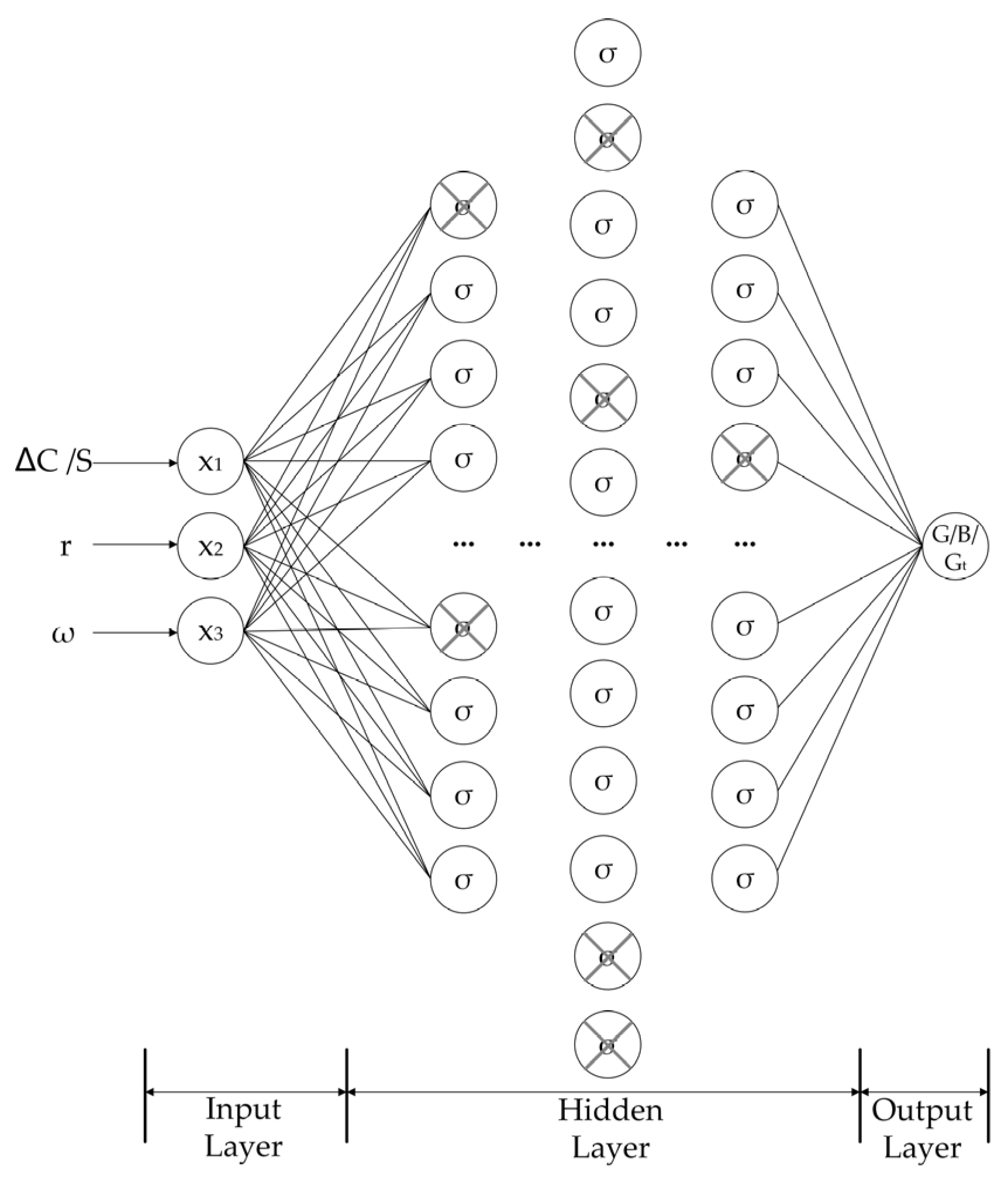
3.6. Artificial Neural Network
3.6.1. Construction of Artificial Neural Network
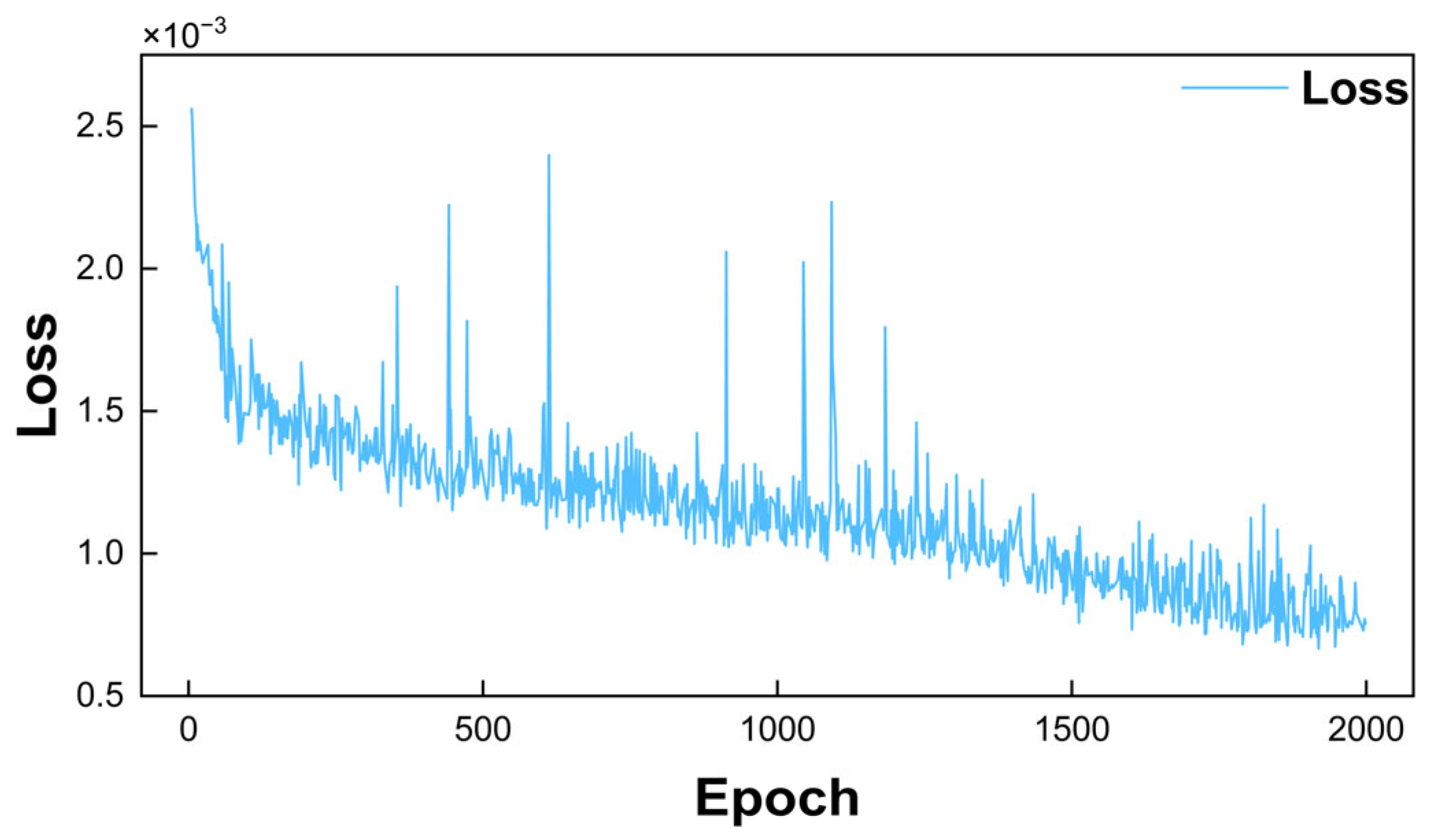
3.6.2. Training of Artificial Neural Network
3.7. Parameter Fitting
3.7.1. Kinetic Parameter Fitting
3.7.2. Crystal Size Distribution Data Processing
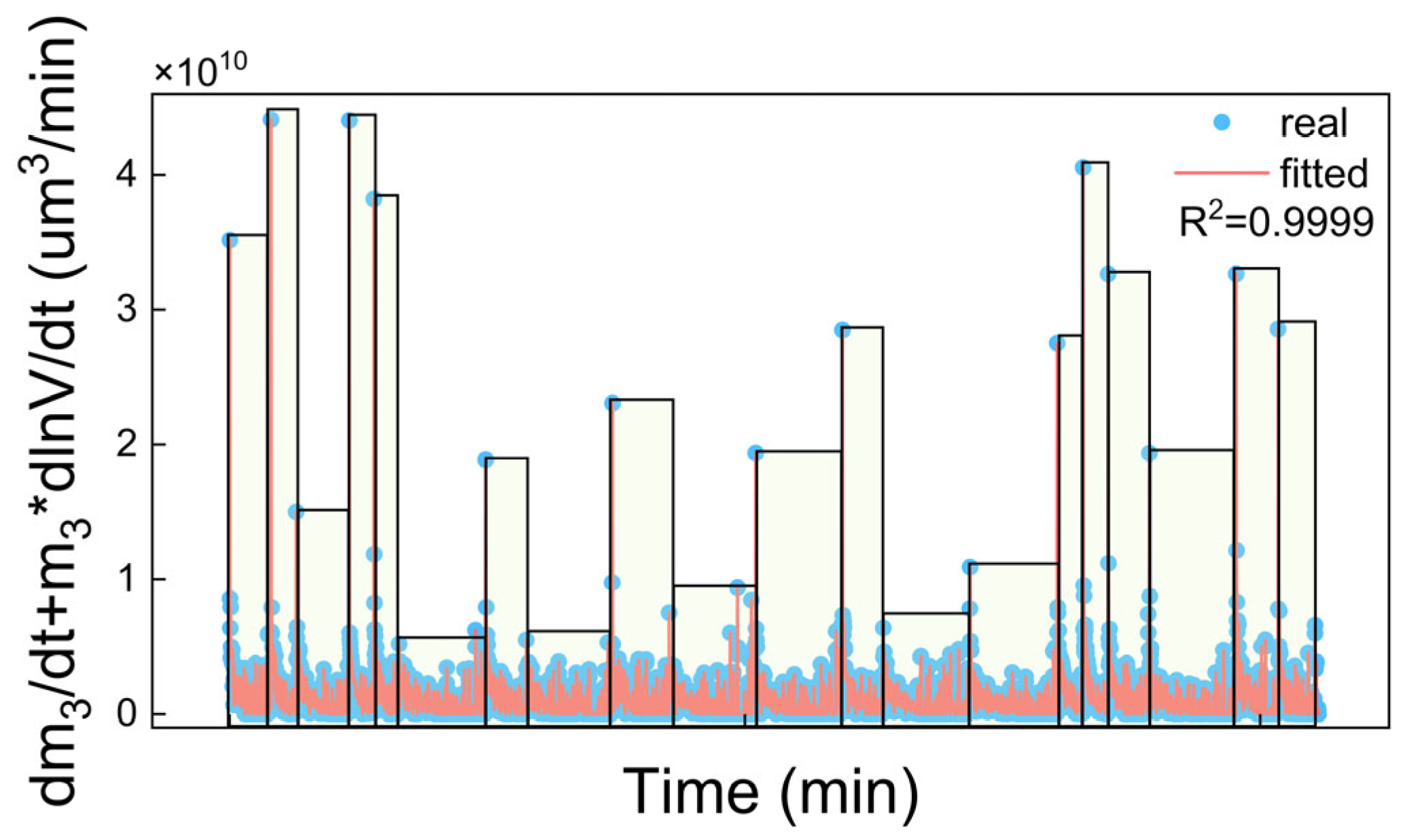
3.7.3. Fitting the Change Rate of Crystal Size Distribution in Process Simulation
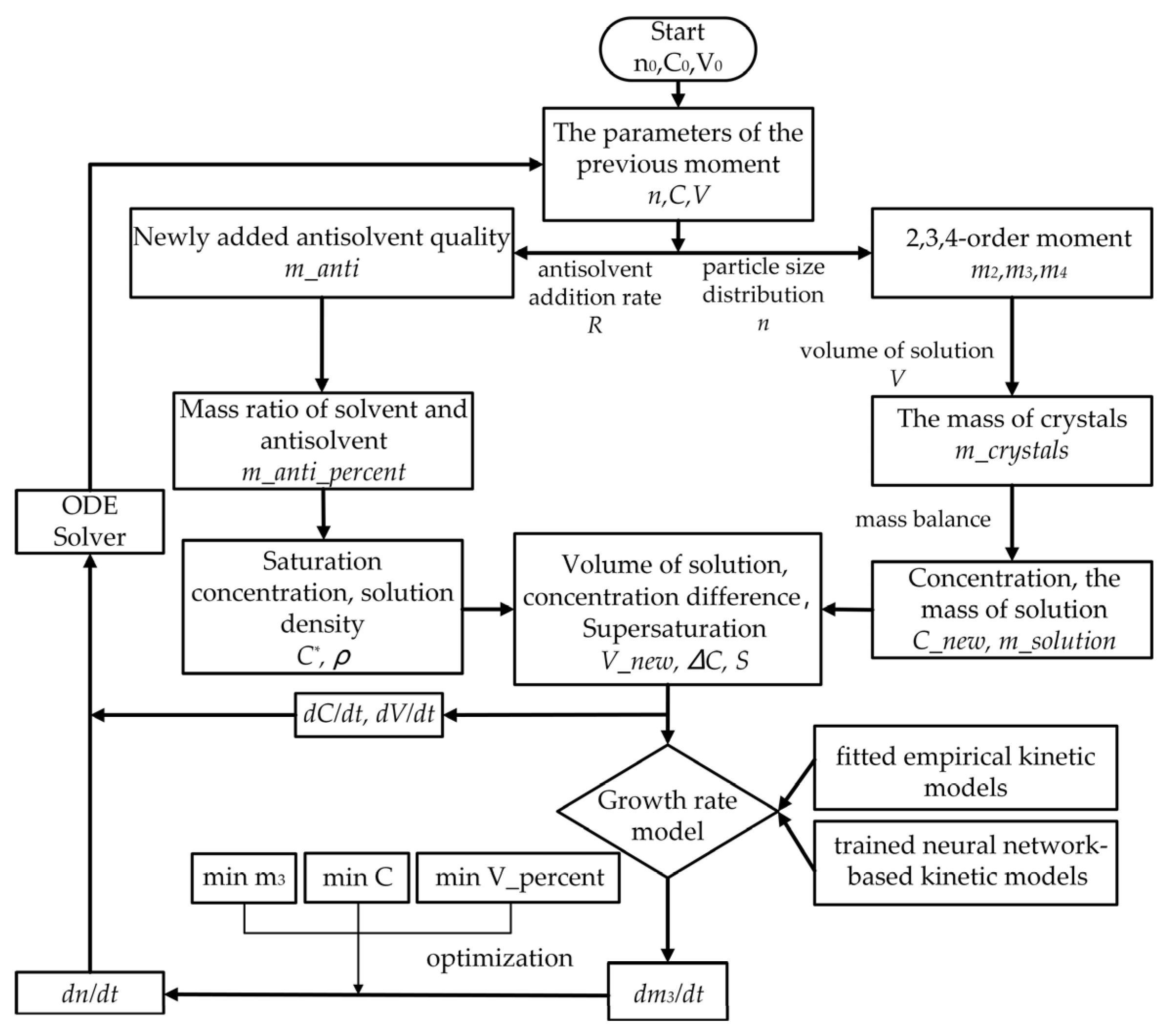
3.8. Process Simulation
4. Results and Discussion
4.1. Kinetic Fitting
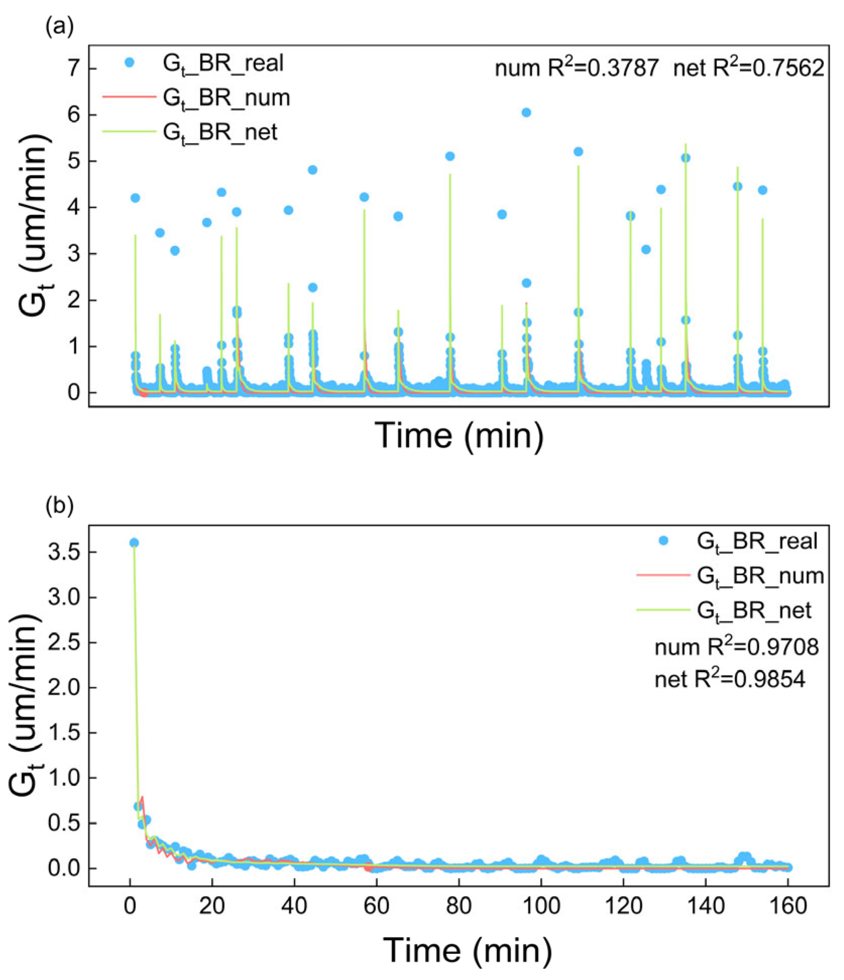
4.1.1. Fitting Results of Growth Rate
- (1)
- Size-dependent growth
- (2)
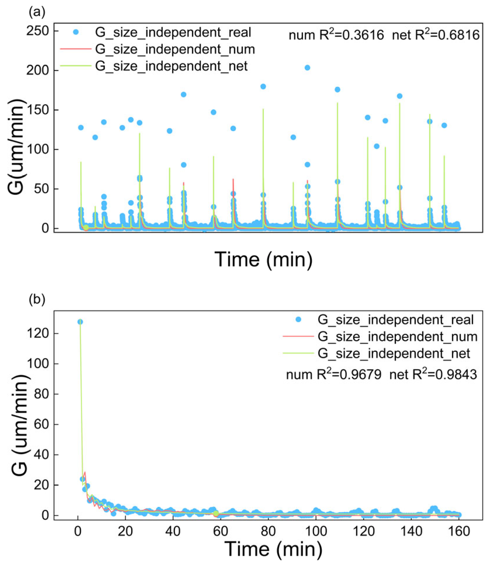
- Size-independent growth
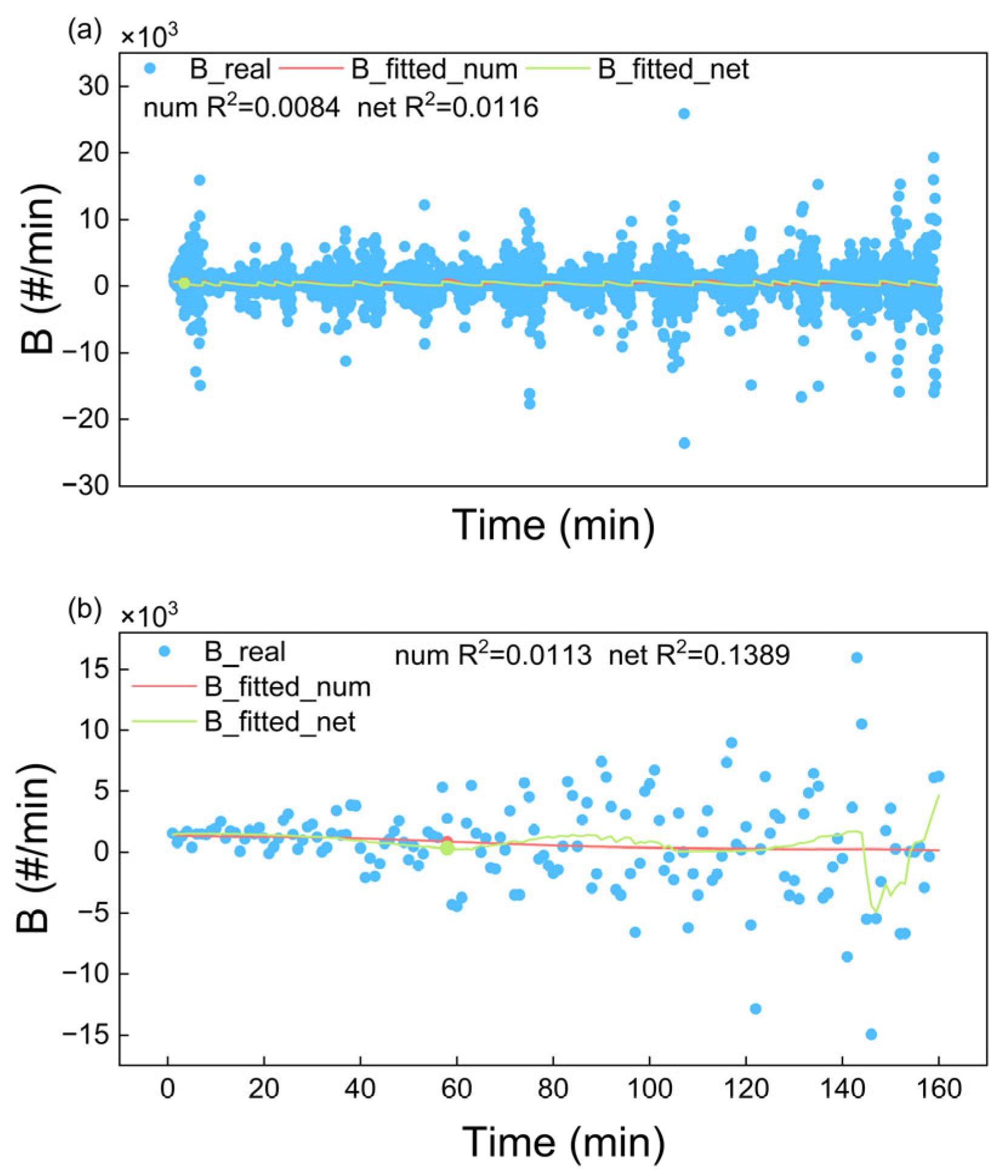
4.1.2. Fitting Results of Nucleation Rate
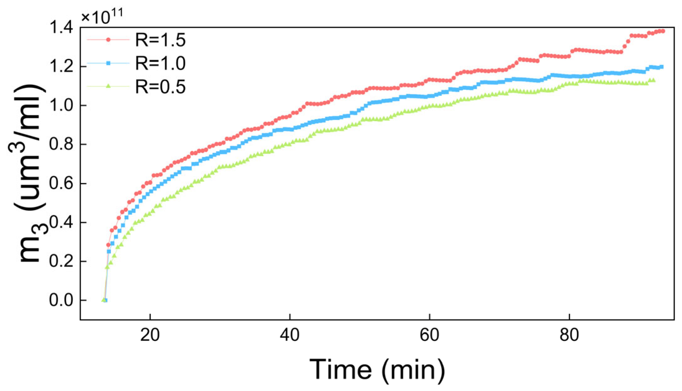
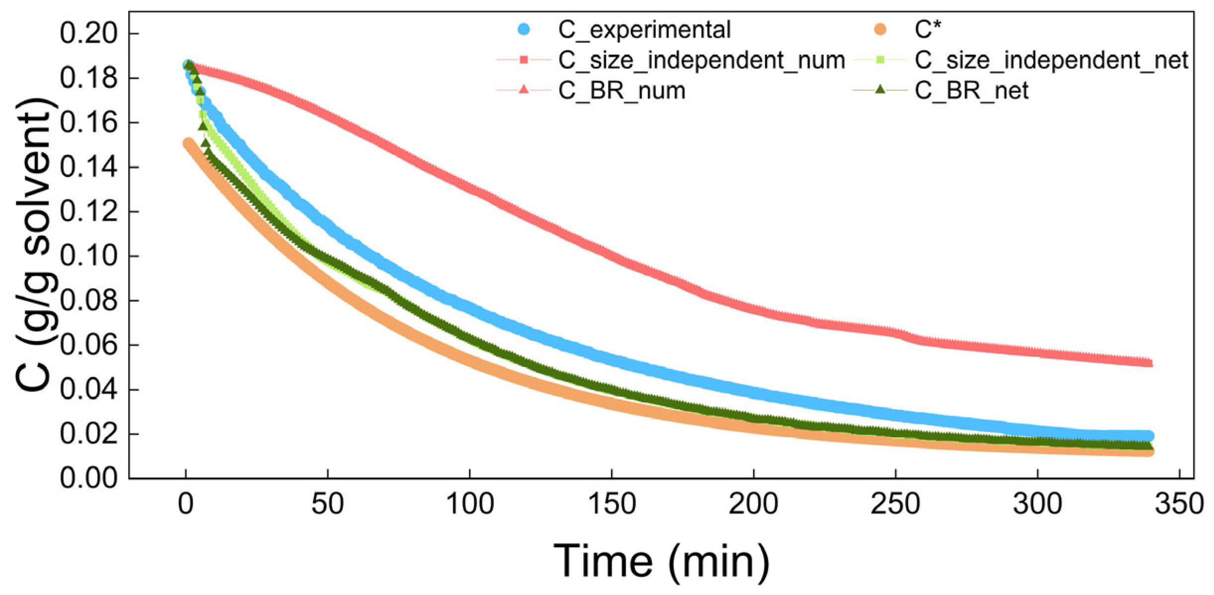
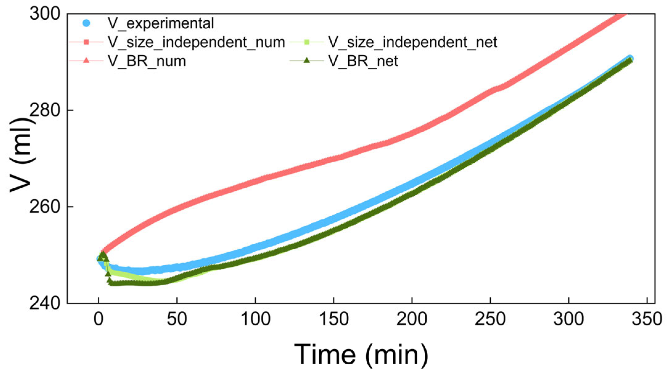
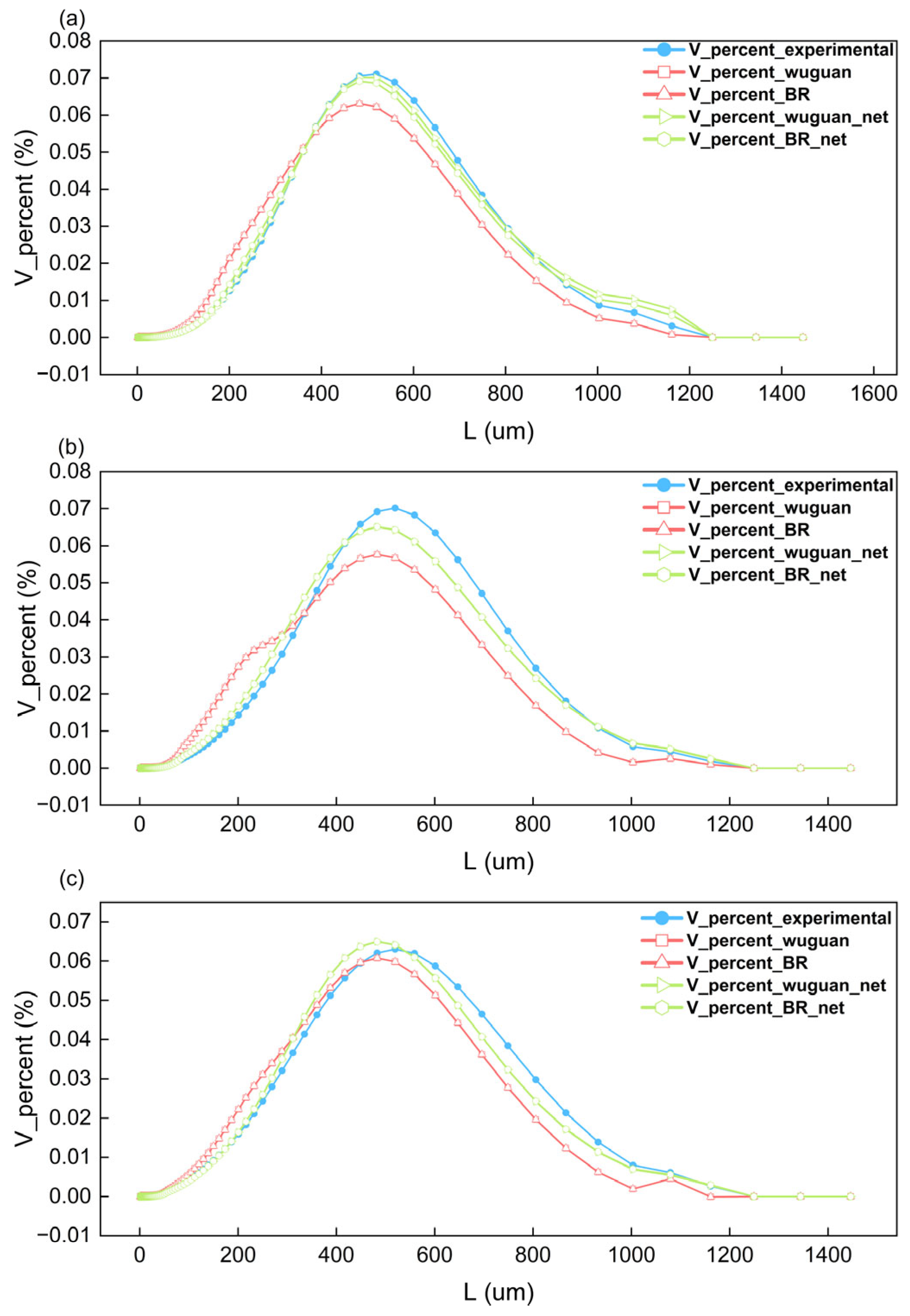
4.2. The Results of Process Simulation
5. Conclusions
Supplementary Materials
Author Contributions
Funding
Data Availability Statement
Conflicts of Interest
References
- Mostafa Nowee, S.; Abbas, A.; Romagnoli, J.A. Antisolvent Crystallization: Model Identification, Experimental Validation and Dynamic Simulation. Chem. Eng. Sci. 2008, 63, 5457–5467. [Google Scholar] [CrossRef]
- Muthancheri, I.; Long, B.; Ryan, K.M.; Padrela, L.; Ramachandran, R. Development and Validation of a Two-Dimensional Population Balance Model for a Supercritical CO2 Antisolvent Batch Crystallization Process. Adv. Powder Technol. 2020, 31, 3191–3204. [Google Scholar] [CrossRef]
- Omar, H.M.; Rohani, S. Crystal Population Balance Formulation and Solution Methods: A Review. Cryst. Growth Des. 2017, 17, 4028–4041. [Google Scholar] [CrossRef]
- Pawar, N.; Agrawal, S.; Methekar, R. Modeling, Simulation, and Influence of Operational Parameters on Crystal Size and Morphology in Semibatch Antisolvent Crystallization of α-Lactose Monohydrate. Cryst. Growth Des. 2018, 18, 4511–4521. [Google Scholar] [CrossRef]
- Ramisetty, K.A.; Pandit, A.B.; Gogate, P.R. Ultrasound-Assisted Antisolvent Crystallization of Benzoic Acid: Effect of Process Variables Supported by Theoretical Simulations. Ind. Eng. Chem. Res. 2013, 52, 17573–17582. [Google Scholar] [CrossRef]
- Jia, S.; Yang, P.; Gao, Z.; Li, Z.; Fang, C.; Gong, J. Recent Progress in Antisolvent Crystallization. Cryst. Eng. Commun. 2022, 24, 3122–3135. [Google Scholar] [CrossRef]
- Abbas, A.; Romagnoli, J.; Widenski, D. Modeling of Crystallization Processes. In Process Systems Engineering; John Wiley & Sons, Ltd.: Hoboken, NJ, USA, 2010; pp. 239–285. ISBN 978-3-527-63120-9. [Google Scholar]
- Rosenbaum, T.; Tan, L.; Dummeldinger, M.; Mitchell, N.; Engstrom, J. Population Balance Modeling To Predict Particle Size Distribution upon Scale-Up of a Combined Antisolvent and Cooling Crystallization of an Active Pharmaceutical Ingredient. Org. Process Res. Dev. 2019, 23, 2666–2677. [Google Scholar] [CrossRef]
- Kumar, R.; Thakur, A.K.; Banerjee, N.; Kumar, A.; Gaurav, G.K.; Arya, R.K. Liquid Antisolvent Crystallization of Pharmaceutical Compounds: Current Status and Future Perspectives. Drug Deliv. Transl. Res. 2023, 13, 400–418. [Google Scholar] [CrossRef]
- Orehek, J.; Češnovar, M.; Teslić, D.; Likozar, B. Mechanistic Crystal Size Distribution (CSD)-Based Modelling of Continuous Antisolvent Crystallization of Benzoic Acid. Chem. Eng. Res. Des. 2021, 170, 256–269. [Google Scholar] [CrossRef]
- Zhou, G.X.; Fujiwara, M.; Woo, X.Y.; Rusli, E.; Tung, H.-H.; Starbuck, C.; Davidson, O.; Ge, Z.; Braatz, R.D. Direct Design of Pharmaceutical Antisolvent Crystallization through Concentration Control. Cryst. Growth Des. 2006, 6, 892–898. [Google Scholar] [CrossRef]
- Trampuž, M.; Teslić, D.; Likozar, B. Process Analytical Technology-Based (PAT) Model Simulations of a Combined Cooling, Seeded and Antisolvent Crystallization of an Active Pharmaceutical Ingredient (API). Powder Technol. 2020, 366, 873–890. [Google Scholar] [CrossRef]
- Lima, F.A.R.D.; Rebello, C.M.; Costa, E.A.; Santana, V.V.; Moares, M.G.F.d.; Barreto, A.G.; Secchi, A.R.; Souza, M.B.d.; Nogueira, I.B.R. Improved Modeling of Crystallization Processes by Universal Differential Equations. Chem. Eng. Res. Des. 2023, 200, 538–549. [Google Scholar] [CrossRef]
- Chen, X.; Wang, L.G.; Meng, F.; Luo, Z.-H. Physics-Informed Deep Learning for Modelling Particle Aggregation and Breakage Processes. Chem. Eng. J. 2021, 426, 131220. [Google Scholar] [CrossRef]
- Wu, G.; Yion, W.T.G.; Dang, K.L.N.Q.; Wu, Z. Physics-Informed Machine Learning for MPC: Application to a Batch Crystallization Process. Chem. Eng. Res. Des. 2023, 192, 556–569. [Google Scholar] [CrossRef]
- Wu, S.; Xia, H. Parameter Identification of Multi-Dimensional PBE Growth Model Based on PINN. In Proceedings of the 2024 43rd Chinese Control Conference (CCC), Kunming, China, 28–31 July 2024; pp. 1372–1377. [Google Scholar]
- Zheng, Y.; Wang, X.; Wu, Z. Machine Learning Modeling and Predictive Control of the Batch Crystallization Process. Ind. Eng. Chem. Res. 2022, 61, 5578–5592. [Google Scholar] [CrossRef]
- Lima, F.A.R.D.; de Moraes, M.G.F.; Barreto, A.G.; Secchi, A.R.; Grover, M.A.; de Souza, M.B. Applications of Machine Learning for Modeling and Advanced Control of Crystallization Processes: Developments and Perspectives. Digit. Chem. Eng. 2025, 14, 100208. [Google Scholar] [CrossRef]
- Tian, Y.; Zhang, Y.; Zhang, H. Recent Advances in Stochastic Gradient Descent in Deep Learning. Mathematics 2023, 11, 682. [Google Scholar] [CrossRef]
- Ojha, V.K.; Abraham, A.; Snášel, V. Metaheuristic Design of Feedforward Neural Networks: A Review of Two Decades of Research. Eng. Appl. Artif. Intell. 2017, 60, 97–116. [Google Scholar] [CrossRef]
- Blazevicius, D.; Grigalevicius, S. A Review of Benzophenone-Based Derivatives for Organic Light-Emitting Diodes. Nanomaterials 2024, 14, 356. [Google Scholar] [CrossRef]
- Dorman, G.; Prestwich, G.D. Benzophenone Photophores in Biochemistry. Biochemistry 1994, 33, 5661–5673. [Google Scholar] [CrossRef]
- Surana, K.; Chaudhary, B.; Diwaker, M.; Sharma, S. Benzophenone: A Ubiquitous Scaffold in Medicinal Chemistry. Med. Chem. Commun. 2018, 9, 1803–1817. [Google Scholar] [CrossRef] [PubMed]
- Heurung, A.R.; Raju, S.I.; Warshaw, E.M. Benzophenones. Dermatitis 2014, 25, 3–10. [Google Scholar] [CrossRef] [PubMed]
- Boscá, F.; Miranda, M.A. New Trends in Photobiology (Invited Review) Photosensitizing Drugs Containing the Benzophenone Chromophore. J. Photochem. Photobiol. B Biol. 1998, 43, 1–26. [Google Scholar] [CrossRef]
- Zhao, W.; He, Z.; Lam, J.W.Y.; Peng, Q.; Ma, H.; Shuai, Z.; Bai, G.; Hao, J.; Tang, B.Z. Rational Molecular Design for Achieving Persistent and Efficient Pure Organic Room-Temperature Phosphorescence. Chem 2016, 1, 592–602. [Google Scholar] [CrossRef]
- Zhang, B.; Song, L.; Feng, C.; Tian, W. Study on Synthesis, Optical Properties and Application of Benzophenone Derivatives. Chem. Sel. 2022, 7, e202203948. [Google Scholar] [CrossRef]
- Ouyang, J.; Na, B.; Xiong, G.; Xu, L.; Jin, T. Corrigendum to “Determination of Solubility and Thermodynamic Properties of Benzophenone in Different Pure Solvents. J. Chem. Eng. Data 2018, 63, 4809–4810. [Google Scholar] [CrossRef]
- Ouyang, J.; Na, B.; Xiong, G.; Xu, L.; Jin, T. Determination of Solubility and Thermodynamic Properties of Benzophenone in Different Pure Solvents. J. Chem. Eng. Data 2018, 63, 1833–1840. [Google Scholar] [CrossRef]
- Azizian, S.; Haydarpour, A. Solubility of Benzophenone in Binary Alkane + Carbon Tetrachloride Solvent Mixtures. J. Chem. Eng. Data 2003, 48, 1476–1478. [Google Scholar] [CrossRef]
- Ouyang, J.; Liu, L.; Zhou, L.; Liu, Z.; Li, Y.; Zhang, C. Solubility, Dissolution Thermodynamics, Hansen Solubility Parameter and Molecular Simulation of 4-Chlorobenzophenone with Different Solvents. J. Mol. Liq. 2022, 360, 119438. [Google Scholar] [CrossRef]
- Hulburt, H.M.; Katz, S. Some Problems in Particle Technology: A Statistical Mechanical Formulation. Chem. Eng. Sci. 1964, 19, 555–574. [Google Scholar] [CrossRef]
- Marchisio, D.L.; Pikturna, J.T.; Fox, R.O.; Vigil, R.D.; Barresi, A.A. Quadrature Method of Moments for Population-Balance Equations. AIChE J. 2003, 49, 1266–1276. [Google Scholar] [CrossRef]
- McGraw, R. Description of Aerosol Dynamics by the Quadrature Method of Moments. Aerosol Sci. Technol. 1997, 27, 255–265. [Google Scholar] [CrossRef]
- Trifkovic, M.; Sheikhzadeh, M.; Rohani, S. Kinetics Estimation and Single and Multi-Objective Optimization of a Seeded, Anti-Solvent, Isothermal Batch Crystallizer. Ind. Eng. Chem. Res. 2008, 47, 1586–1595. [Google Scholar] [CrossRef]
- Ashraf, A.B.; Rao, C.S. Multiobjective Temperature Trajectory Optimization for Unseeded Batch Cooling Crystallization of Aspirin. Comput. Chem. Eng. 2022, 160, 107704. [Google Scholar] [CrossRef]
- Widenski, D.J.; Abbas, A.; Romagnoli, J.A. Use of Predictive Solubility Models for Isothermal Antisolvent Crystallization Modeling and Optimization. Ind. Eng. Chem. Res. 2011, 50, 8304–8313. [Google Scholar] [CrossRef]
- Liu, P.; Yang, L.; Ma, Y.; Zhang, Y.; Wang, H.; Cheng, J.; Yang, C. Continuous Antisolvent Crystallization of L-Histidine: Impact of Process Parameters and Kinetic Estimation. Ind. Eng. Chem. Res. 2024, 63, 2831–2841. [Google Scholar] [CrossRef]
- Bransom, S.H. Factors in the Design of Continuous Crystallizer. Br. Chem. Eng. 1960, 5, 838–843. [Google Scholar]
- Canning, T.F.; Randolph, A.D. Some Aspects of Crystallization Theory: Systems That Violate McCabe’s Delta L Law. AIChE J. 1967, 13, 5–10. [Google Scholar] [CrossRef]
- Mydlarz, J.; Jones, A.G. On Modelling the Size-Dependent Growth Rate of Potassium Sulphate in an Msmpr Crystallizer. Chem. Eng. Commun. 1990, 90, 47–56. [Google Scholar] [CrossRef]
- Mydlarz, J.; Jones, A.G. On the Estimation of Size-Dependent Crystal Growth Rate Functions in MSMPR Crystallizers. Chem. Eng. J. Biochem. Eng. J. 1993, 53, 125–135. [Google Scholar] [CrossRef]
- Zhao, W.; Li, B.; Liu, S.; Deng, Y.; Zhang, R.; Jiang, Y. Kinetic Study of Complicated Anti-Solvent and Cooling Crystallization of Disodium 5′-Ribonucleotide. Particuology 2023, 73, 103–112. [Google Scholar] [CrossRef]
- Trifkovic, M.; Sheikhzadeh, M.; Rohani, S. Multivariable Real-Time Optimal Control of a Cooling and Antisolvent Semibatch Crystallization Process. AIChE J. 2009, 55, 2591–2602. [Google Scholar] [CrossRef]


| Model | kg/ks | a/α | b/β | γ | g | g1 | g2 |
|---|---|---|---|---|---|---|---|
| BR | 0.1397 | 0.6103 | - | - | 14.5050 | −1.0290 | 86.9987 |
| CR | 0.1606 | 0.0846 | - | - | 13.7161 | −0.9428 | 87.3030 |
| MJ2 | 0.2034 | −0.0177 | - | - | 10.5024 | −0.6476 | 88.3385 |
| MJ3 | 0.2067 | 0.0193 | 0.6507 | - | 11.8111 | −0.6652 | 87.0589 |
| Size independent | −0.0312 | - | - | - | 14.9793 | −1.8738 | 90.8026 |
| Nucleation Rate | −25.5839 | 10.7180 | 0.0832 | 200.3924 | - | - | - |
| Model | 20 Sets of Experimental Data | 1 Set of Experimental Data | ||
|---|---|---|---|---|
| Num R2 | Net R2 | Num R2 | Net R2 | |
| BR | 0.3787 | 0.7562 | 0.9708 | 0.9854 |
| CR | 0.3742 | 0.6856 | 0.9711 | 0.9855 |
| MJ2 | 0.3499 | 0.6867 | 0.9712 | 0.9854 |
| MJ3 | 0.3639 | 0.6696 | 0.9712 | 0.9858 |
| Size-independent | 0.3616 | 0.6816 | 0.9679 | 0.9843 |
| Nucleation Rate | 0.0084 | 0.0116 | 0.0113 | 0.1389 |
| Model | Concentration | Volume | CSD at 15 min | CSD at 90 min | CSD at 180 min | |||||
|---|---|---|---|---|---|---|---|---|---|---|
| Num | Net | Num | Net | Num | Net | Num | Net | Num | Net | |
| Size_independent | 0.0052 | 0.9296 | 0.2963 | 0.9824 | 0.9560 | 0.9981 | 0.9147 | 0.9879 | 0.9471 | 0.9890 |
| BR | 0.0052 | 0.9196 | 0.2963 | 0.9796 | 0.9560 | 0.9964 | 0.9147 | 0.9882 | 0.9471 | 0.9875 |
| CR | 0.0052 | 0.8968 | 0.2963 | 0.9715 | 0.9560 | 0.9957 | 0.9147 | 0.9880 | 0.9471 | 0.9873 |
| MJ2 | 0.0052 | 0.9426 | 0.2963 | 0.9853 | 0.9560 | 0.9829 | 0.9147 | 0.9854 | 0.9471 | 0.9787 |
| MJ3 | 0.0052 | 0.9391 | 0.2963 | 0.9803 | 0.9560 | 0.9510 | 0.9147 | 0.9760 | 0.9471 | 0.9617 |
Disclaimer/Publisher’s Note: The statements, opinions and data contained in all publications are solely those of the individual author(s) and contributor(s) and not of MDPI and/or the editor(s). MDPI and/or the editor(s) disclaim responsibility for any injury to people or property resulting from any ideas, methods, instructions or products referred to in the content. |
© 2025 by the authors. Licensee MDPI, Basel, Switzerland. This article is an open access article distributed under the terms and conditions of the Creative Commons Attribution (CC BY) license (https://creativecommons.org/licenses/by/4.0/).
Share and Cite
Dong, Y.; Xuanyuan, S.; Xie, C.; Sun, Y.; Zhou, X.; Wang, Y. Neural Network-Based Kinetic Model for Antisolvent Crystallization of Benzophenone: Construction, Validation, and Mechanistic Interpretation. Crystals 2025, 15, 464. https://doi.org/10.3390/cryst15050464
Dong Y, Xuanyuan S, Xie C, Sun Y, Zhou X, Wang Y. Neural Network-Based Kinetic Model for Antisolvent Crystallization of Benzophenone: Construction, Validation, and Mechanistic Interpretation. Crystals. 2025; 15(5):464. https://doi.org/10.3390/cryst15050464
Chicago/Turabian StyleDong, Yafei, Shutian Xuanyuan, Chuang Xie, Ying Sun, Xiaomeng Zhou, and Yuanhang Wang. 2025. "Neural Network-Based Kinetic Model for Antisolvent Crystallization of Benzophenone: Construction, Validation, and Mechanistic Interpretation" Crystals 15, no. 5: 464. https://doi.org/10.3390/cryst15050464
APA StyleDong, Y., Xuanyuan, S., Xie, C., Sun, Y., Zhou, X., & Wang, Y. (2025). Neural Network-Based Kinetic Model for Antisolvent Crystallization of Benzophenone: Construction, Validation, and Mechanistic Interpretation. Crystals, 15(5), 464. https://doi.org/10.3390/cryst15050464