Abstract
Machine learning-based image recognition is employed to investigate the annihilation dynamics of umbilic defects induced in systems of nematic liquid crystals doped with nanoparticles. A machine learning methodology based on a YOLO algorithm is trained and optimized to identify defects of strength s = ±1 and determine their trajectories during the annihilation process of umbilics of opposite sign. Universal scaling laws describing the distance between two defects as a function of time to annihilation are determined, and average scaling exponents α are calculated for an ensemble of events. It is observed that the defect annihilation scaling exponents deviate from the theoretically predicted value of α = 1/2 when nanoparticles of varying size and concentration are introduced to the system. Scaling laws of the form D~tα do not yield the typical square-root law normally observed, but the experiments suggest a decrease in the exponent to saturation values of approximately α = 0.38 ± 0.01 as the size, particle concentration, and mass concentration of the nanoparticles is increased. Interestingly, the defect density itself is not affected, which implies that the nanoparticles do not act as defect formation sites.
1. Introduction
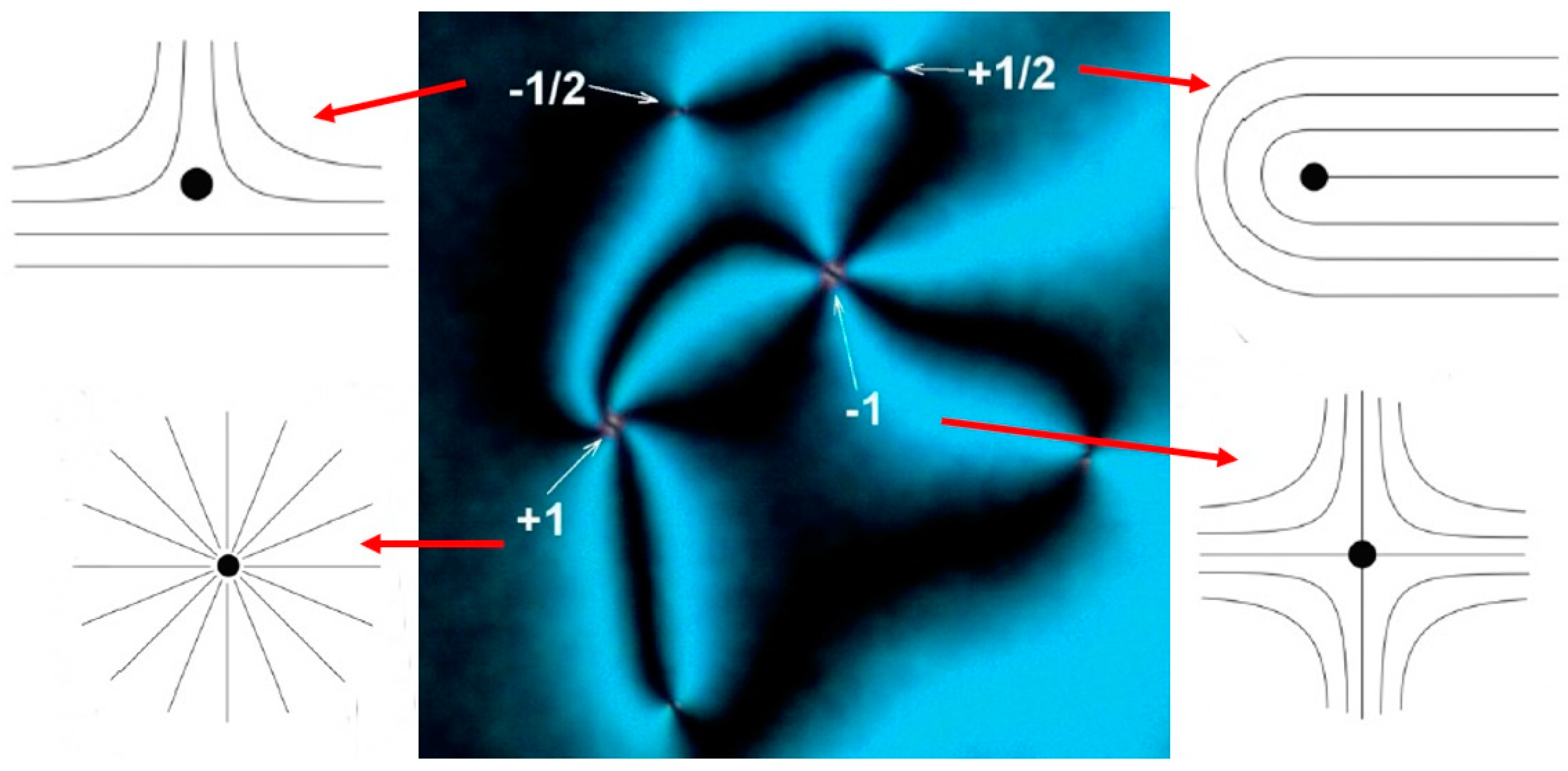
The coarsening dynamics of nematic liquid crystal topological defects have been studied by a number of authors ever since an analogy to cosmological defects was formulated [1]. Investigations have been carried out both experimentally and via simulations and theory. Experimental studies have included string defects [1,2,3,4] and defect loops [4,5] but were mainly concentrated on the annihilation of defect pairs of opposite sign and equal strength [6,7,8], as they are found in the schlieren textures of the nematic phase after a temperature or pressure quench from the isotropic liquid. These defects can have a strength of s = ±1/2 or s = ±1: they are singularities in the nematic director field and are illustrated in Figure 1, both as a texture observed experimentally via polarizing microscopy and schematically. In an ideal, infinite sample, the total sum over all defects will be equal to zero.
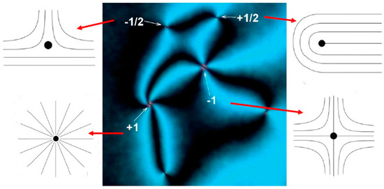
Figure 1.
Nematic schlieren texture obtained after a temperature quench from the isotropic liquid between crossed polarizers, illustrating the four singular defects with strengths of s = ±1/2 and s = ±1, also shown schematically (reproduced from ref. [9] with permission).
These types of topological defects arise in many physical systems, such as in cosmology [10], super-fluids [11], solid-state materials [12], active matter [13], and biological [14] and living systems [15]. It was found that liquid crystals are simple model systems to study the mechanisms and dynamics of symmetry breaking through phase transitions, during which topological defects are formed [16].
As liquid crystals are elastic fluids, the defect dynamics can be described by continuum theory, provided that the defect motion is overdamped and adiabatic [17]. Previous experimental work has shown that the dynamics of defect annihilation comprise a complex combination of elastic attractions, viscous drag forces, backflow effects, director configurations, and cell confinement [18]. In this analysis, however, only elastic attractions and viscous drag forces are considered, and elasticity is treated in the one-constant approximation K11 = K22 = K33 = K, i.e., splay-, twist-, and bend-elastic constants are taken as equal in magnitude.
Considering two defects of strength s1 and s2 separated by distance D, the attractive elastic force is given as follows:
The drag force for a defect of strength s with velocity v in a film with no flow is given as follows [19]:
where γ is the rotational viscosity and Er is the Eriksen number, equal to the ratio of viscous to elastic forces.
Equating the elastic and drag forces yields a terminal velocity of defects as follows:
Integration gives the following:
and thus,
The distance between two annihilating defects therefore follows a simple scaling law of the following form:
where t0 is the time of annihilation and α is the scaling exponent, which takes a value of 1/2 according to the simple considerations above. A more explicit theoretical treatment, as well as computer simulations [20,21,22,23,24], support the scaling law of D(t)~(t0 − t)1/2, which is indeed also found experimentally [6,7,8].
The symmetry-breaking phase transition from isotropic to liquid crystal is often induced by temperature quenches, as in the case of the nematic phase [6], but also for smectic C [25] or nematic polymers [26,27]. Equivalent is the use of another intensive variable of state: pressure quenches to induce the symmetry breaking phase transition and the formation of defects [1,4,5,6]. We here utilize a somewhat different mechanism to induce defects in the form of the application of electric fields to a dielectrically negative nematic liquid crystal subjected to homeotropic boundary conditions—the Freedericksz transition, as it is commonly called. The director switches from a homeotropic to planar orientation, while the substrates provide no in-plane directionality and thus cause a large number of defects to be formed. These defects are called umbilics, and they are not singularities in the director field [28,29,30]. Nevertheless, they represent very localized regions of escape, where the director reorients parallel to the electric field, while the in-plane component of the director rotates through ±2π. This resembles closely the s = ±1 defects, except that the parallel alignment of the core matches smoothly onto the homeotropic surface anchoring instead of ending in singular points. The scaling laws of defect annihilation are equivalent to those of the schlieren defects discussed above, which has been demonstrated in a number of experiments [7,8,31,32] with a varying range of external parameters such as applied electric field amplitude and frequency, cell gap, and temperature, as well as nematic LC material. The advantage of using this methodology to induce defects lies in the fact that a much cleaner system of defects is obtained with only s = +1 and s = −1 defects being present.
In all cases of experimental, theoretical, and simulation work for various defect generating methods as well as different liquid crystal materials and external applied conditions, the above scaling law D(t)~(t0 − t)1/2 was confirmed to hold and is thus seen to be universal. In this paper, we investigated the defect annihilation and its corresponding scaling exponent for a nematic liquid crystal with dispersed nanospheres at varying concentrations and sizes. The experimental results appear to indicate a deviation from universality, and it would be of much interest to see theoretical and simulation work investigating this problem further to shed further light on this issue.
2. Experimental
2.1. Materials and Experimental Data
The nematic liquid crystal used in this investigation was N-(4-Methoxybenzylidene)-4-butylaniline (MBBA) from Synthon Chemicals, Bitterfeld-Wolfen, Germany, which was combined with varying amounts of barium titanate nanoparticles of differing sizes between 45 and 500 nm (Nanografi, Jena, Germany). Both materials were used as received. The liquid crystal MBBA has a negative dielectric anisotropy of approximately Δε ≈ −0.75 [33]. Dispersions were made by mixing the nanospheres into MBBA with isopropanol at (i) varying mass concentrations from 0.01 to 0.4% for a constant nanosphere diameter of 280 nm (thus varying the particle concentration from 0.00006 to 0.003%, assuming spherical particles of uniform density), (ii) varying nanosphere size from 45 to 500 nm at a constant particle concentration of 0.0002% (thus varying the mass density from 0.00015 to 0.2%), and (iii) varying nanosphere size from 45 to 500 nm at constant mass concentration of 0.1% (thus varying the particle concentration from 0.15 to 0.0001%). After solvent evaporation and sonification of the dispersions for 15 min, the materials were filled into ITO-coated Hele–Shaw cells of 15 μm thickness via capillary action in the nematic state at room temperature.
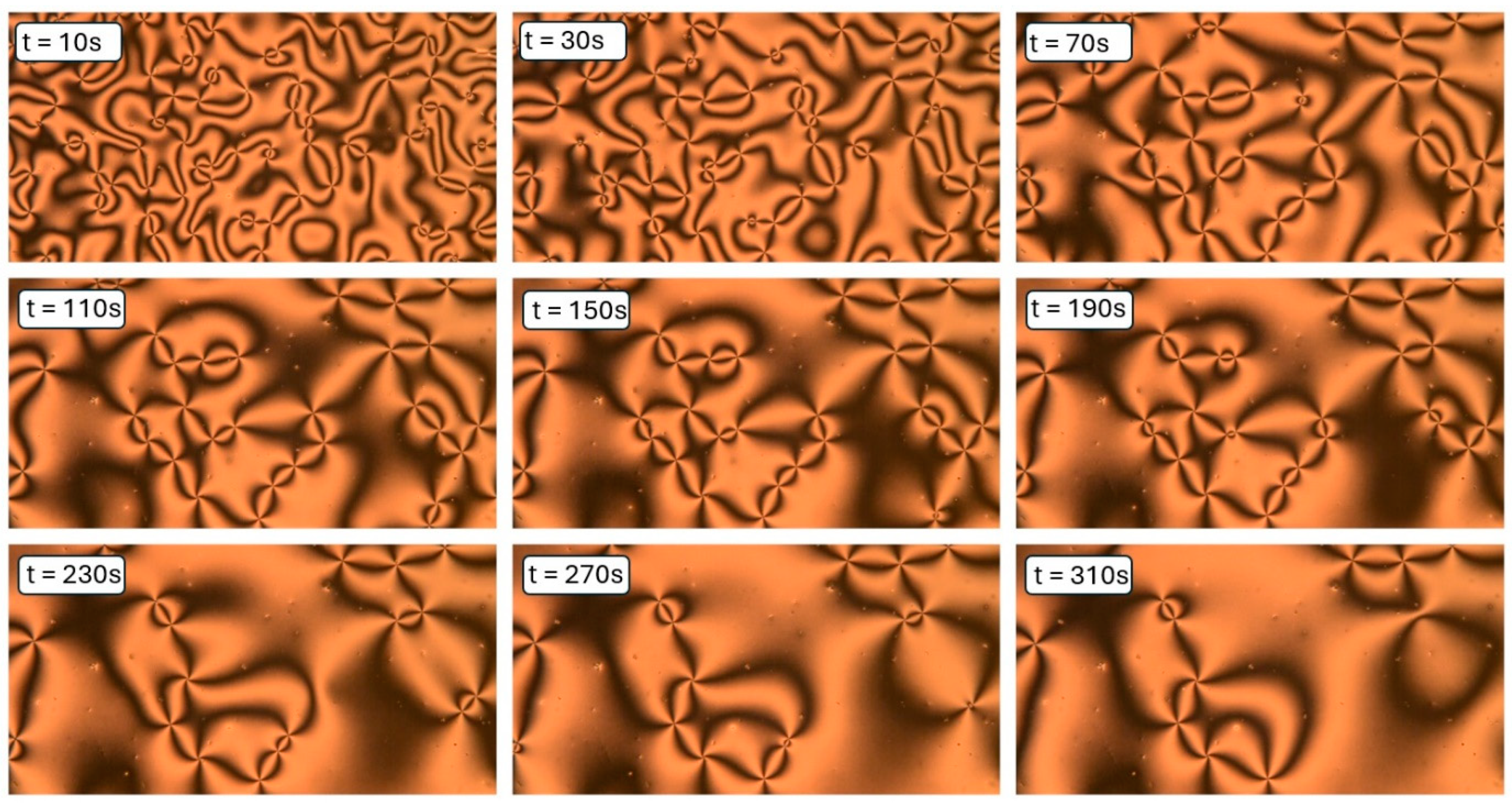
Defects were induced through the application of electric fields well above the Freedericksz threshold at a voltage amplitude of 20 V peak-to-peak with a frequency of 50 kHz (Agilent 33220A function generator and in-house built power amplifier). Defect formation and annihilation were followed using polarizing microscopy (Leica Optipol) in combination with a digital video camera (UI-3360CP-C-HQ, uEye Gigabit Ethernet) at a frame rate of 30 frames per second and resolution of 2048 × 1088 pixels, corresponding to 1546 × 821 μm. The transient defect formation process lasted about 3 s, and the following annihilation process was recorded for at least 3 min (180 s). Figure 2 shows an exemplary time series during defect annihilation of a MBBA/370 nm particle system. Many defect annihilation events can be observed over time, while the defect density decreases.
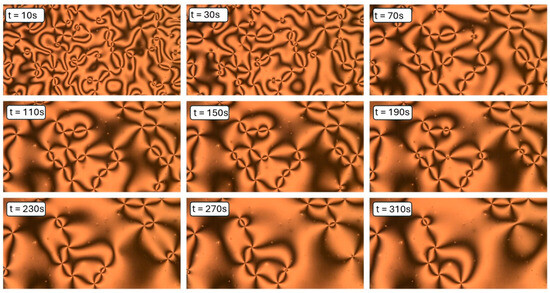
Figure 2.
Annihilation of umbilic defects, exemplarily depicted as a time series for a sample of MBBA with 370 nm nanoparticles at a mass concentration of 0.1%.
Time series of frames extracted from video sequences therefore offer a large number of defect pairs that can be analyzed simultaneously, if the individual defects can be recognized automatically. To this end, a machine learning algorithm was utilized.
2.2. Computer Vision and Image Recognition
To detect the defects in the videos taken, a machine learning architecture called YOLOv5 (by Ultralytics) was used. YOLOv5, which is short for “You Only Look Once version 5”, is an object detection algorithm developed using PyTorch 2.1.2 that enables fast custom object detection. In general, the YOLOv5 algorithms consist of three parts: the backbone, the neck, and the head. The backbone of the YOLOv5 model is a convolutional neural network that aggregates and forms image features at different granularities, i.e., it detects different objects in images provided. The neck is a series of layers to mix and combine image features to pass them forward to prediction, and the head consumes features from the neck, classifies the detected objects, and encases them in bounding boxes. The architecture comes with four prebuilt models, with near-identical methods of operation, differing only in the size of the models themselves: YOLOv5s (small), YOLOv5m (medium), YOLOv5l (large), YOLOv5x (extra-large). The small YOLOv5 model consists of 283 mostly convolutional layers, while the extra-large model consists of 604 layers. YOLOv5 is an object detection algorithm that is well known due to its fast object detection and high accuracy [34]. From testing the various model sizes that are available, it was concluded that YOLOv5s was sufficient to produce a reasonable precision for our anticipated application while maintaining fast inference times. The YOLOv5 models are pretrained on many different commercially available datasets, such as COCO—Common Objects in Context. However, since topological defects are not commonly found objects such as cats and dogs are, the models needed to be manually trained on a custom dataset, as discussed below.
To train YOLOv5 to recognize the topological defects, a labelled dataset of nematic 4-fold defects was assembled. This was done using an online tool called Roboflow, which enables drawing bounding boxes around objects in images and labelling each class of objects. A total of 380 images were processed via the online platform Roboflow in order to use the Roboflow Annotate tool; this allowed each defect to be classified and manually labelled with a bounding box. Within Roboflow, the training images were then augmented and preprocessed to provide the model with more data; a random selection of images was rotated, flipped, or divided into four. To achieve maximal accuracy in the detection of the defect positions, care was taken during the labelling process. The bounding boxes were made as small as possible without generating oversight of defects, and the defect “singularity” was centered within each bounding box. Testing the models produced by YOLOv5 on different versions of the labelled dataset over 100 epochs demonstrated that the tighter bounding boxes were more suitable for purpose within this investigation.
To quantify the tests, precision and recall were calculated, which are performance metrics defined as follows:
and
where tp are true positives, fp are false positives, and fn are false negatives. A higher precision implies that an image recognition algorithm returns more relevant results than irrelevant ones. A higher recall means that an algorithm returns most of the relevant results.
Loss scores are also used to evaluate the success of an object detection model [35]. For example, in YOLOv5, the box loss measures how successfully bounding boxes locate the centers and areas of objects. Class, or CLS, loss measures to what degree a model misclassifies objects, which is irrelevant here, as we only have one class. Thus, class loss is equal to zero. Object loss gives a score of how probable it is that an object resides within a predicted bounding box [36]. An exemplary set of metrics is depicted in Figure 3 over a training period of 100 epochs.
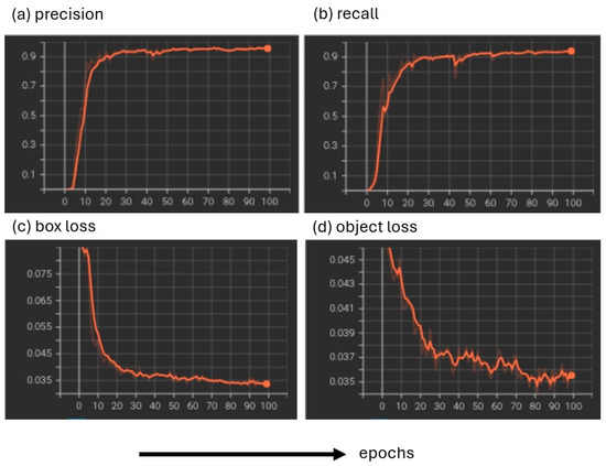
Figure 3.
Exemplary demonstration of the metrics to optimize the object recognition algorithm over 100 epochs: (a) precision, (b) recall, (c) box loss, and (d) object loss.
The so-called ‘best’ weights were extracted, which optimized precision vs. recall and were then used to analyze videos of defects. These videos were sped up by three times to reduce runtime, which was adequate given the large number of frames per second. They were also cropped to remove the sections prior to and including defect formation, concentrating on defect annihilation.
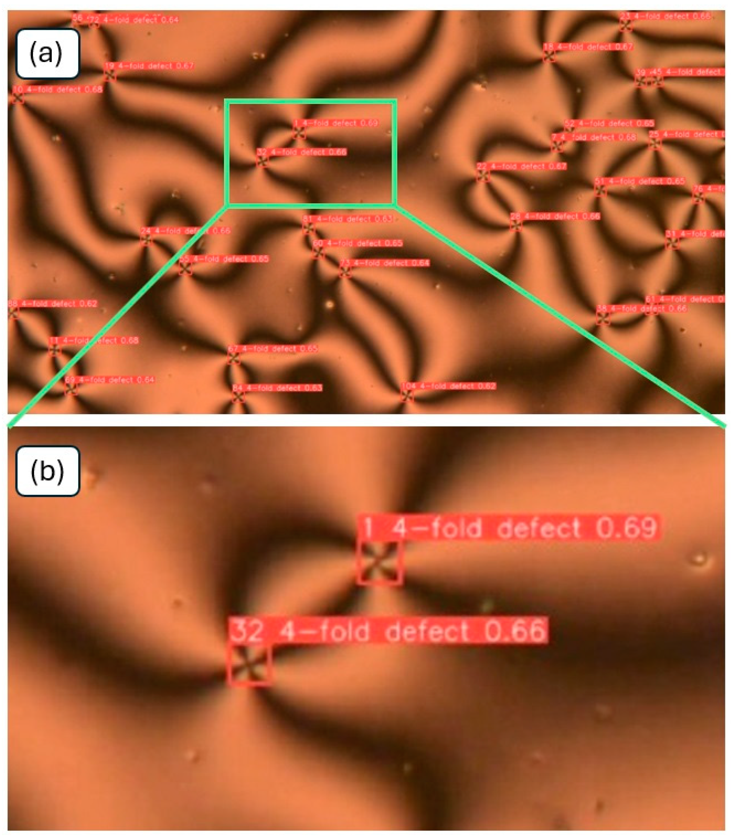
DeepSORT (Simple Online and Realtime Tracking with a Deep association metric) is an object tracking software [37]. A notebook in Google Colab was used with DeepSORT in order to track the defects in the videos, analyzing them on a per-frame basis and producing further videos showing bounding boxes on the defects with confidence levels, as depicted in Figure 4. The confidence level here is of the order of 0.65, which is sufficient, as only one class of defects is studied. For other cases, this could be improved through the use of larger training datasets.
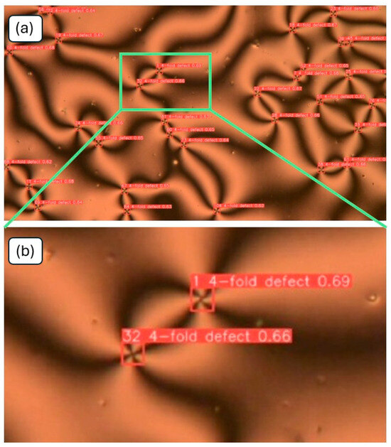
Figure 4.
(a) Test data illustrating that the trained algorithm not only recognizes the defects with excellent accuracy but (b) also places the defect “singularity” in the center of the bounding box, which guarantees highly accurate (x,y)-positions of the tracked defects. The information for each defect is the identification number, the class (here, only 4-fold defects), and the confidence level.
By observing the video with tracked defects, appropriate defects within an annihilating pair were selected, and the distance D(t) between annihilating defect pairs was calculated as a function of time.
3. Experimental Results and Discussion
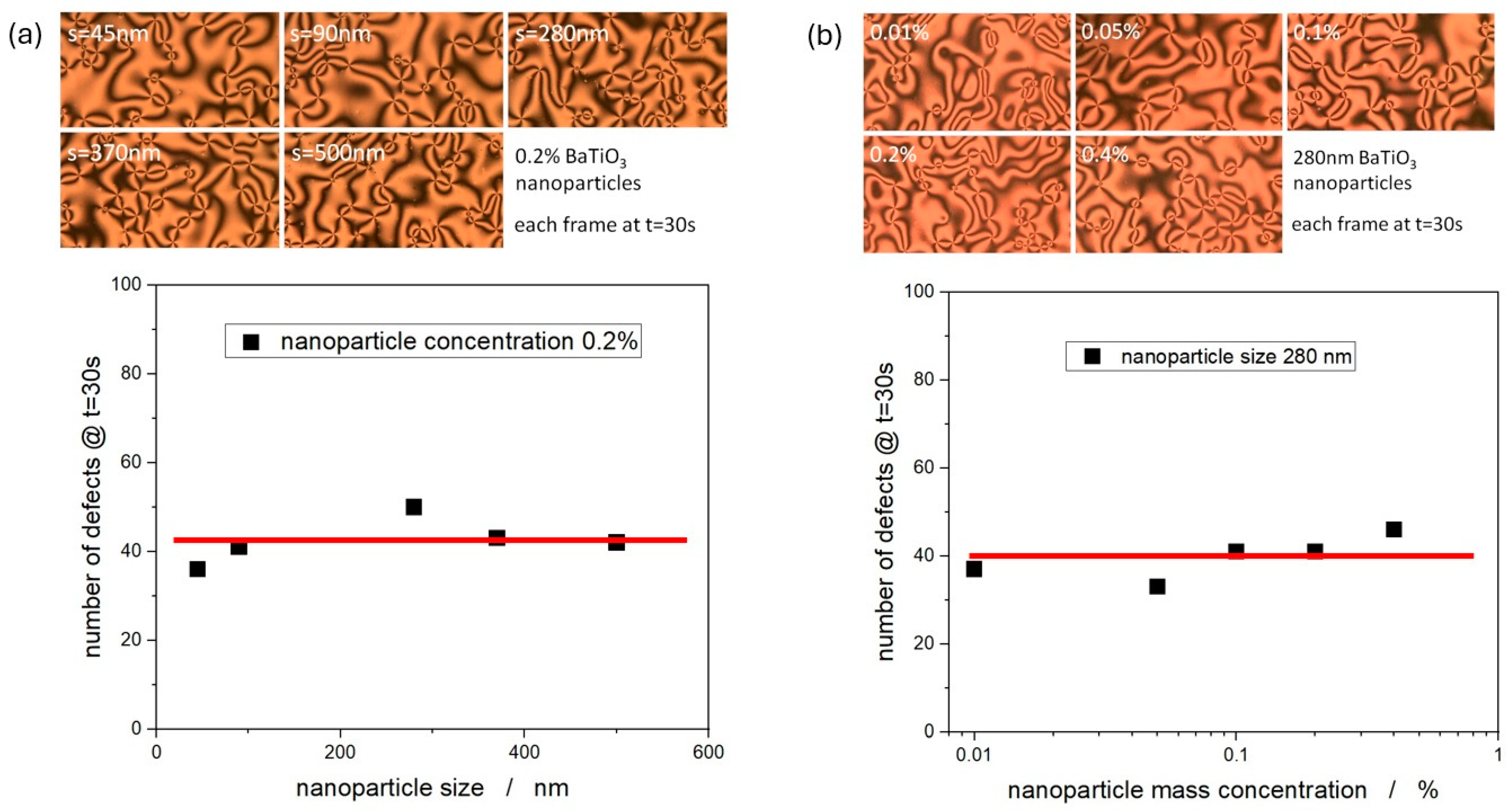
Firstly, it should be mentioned that for consecutive measurement series, defects are not formed in the same locations for each experiment. Nevertheless, this does not imply that there are no nanoparticles at the center of the defects because the former are generally attracted to defects and interfaces. Given the size of the nanoparticles employed, this cannot be verified using optical microscopy. At first, the defect density, i.e., the number of defects per unit area, was investigated for varying nanoparticle sizes at a constant concentration, as well as varying concentrations at a constant particle size. Some exemplary texture series are depicted in Figure 5 for varying the particle size from 45 nm to 500 nm at a concentration of 0.2% (part (a)) and for varying the nanoparticle concentration from 0.01% to 0.4% for a constant particle size of 280 nm (part (b)). In each case, the frame at time t = 30 s is selected for comparison. It is interesting to note that the defect density is almost constant and independent of nanoparticle size and nanoparticle mass concentration.

Figure 5.
Textures at t = 30 s and corresponding number of defects observed (a) as a function of nanoparticle size at a concentration of 0.1% and (b) nanoparticle mass concentration for a particle size of 280 nm.
This implies that the addition of nanoparticles neither appears to influence the defect formation nor the attractive force between the defects. At the same time, the defect density ρ(d,c,t) = ρ(t), with d being the particle size and c being the particle concentration, and in this particular case analyzed above, ρ(t = 30 s) = (33 ± 4) mm−2.
Figure 6 is an exemplary demonstration of defect distance acquisition and subsequent determination of the defect annihilation exponent α from the obtained position data acquired via machine learning as a function of time. In Figure 6a, the original data D(t) are depicted, which are clearly described by a nonlinear relationship D(t)~(t0 − t)α. The annihilation exponent can then be calculated from a log–log representation, which exhibits a linear scaling regime after some time following the application of the electric field. At early times, the relation is not suitable for analysis because of the convolution of two simultaneous processes: defect formation and defect annihilation.
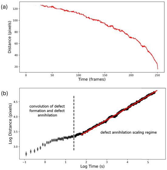
Figure 6.
(a) Original data of D(t), determined via machine learning, and (b) log–log representation for the determination of the annihilation exponent α from the slope of the linear scaling regime.
It should be pointed out that this linear scaling regime is observed for all of the subsequent measurement series, but care needs to be taken to avoid the regime of overlap between formation and annihilation of defects. This way, we could analyze between 6 to 40 defect pairs for each of the individual nematic nanoparticle dispersions. Outliers, such as defects that become trapped with dust contamination within the liquid crystal, were removed from the dataset considering the Chauvenet criterion, which defines an acceptable scattering of values around the mean value from N measurements. This is a widely accepted and soft-touch approach to identify outliers, even for small datasets.
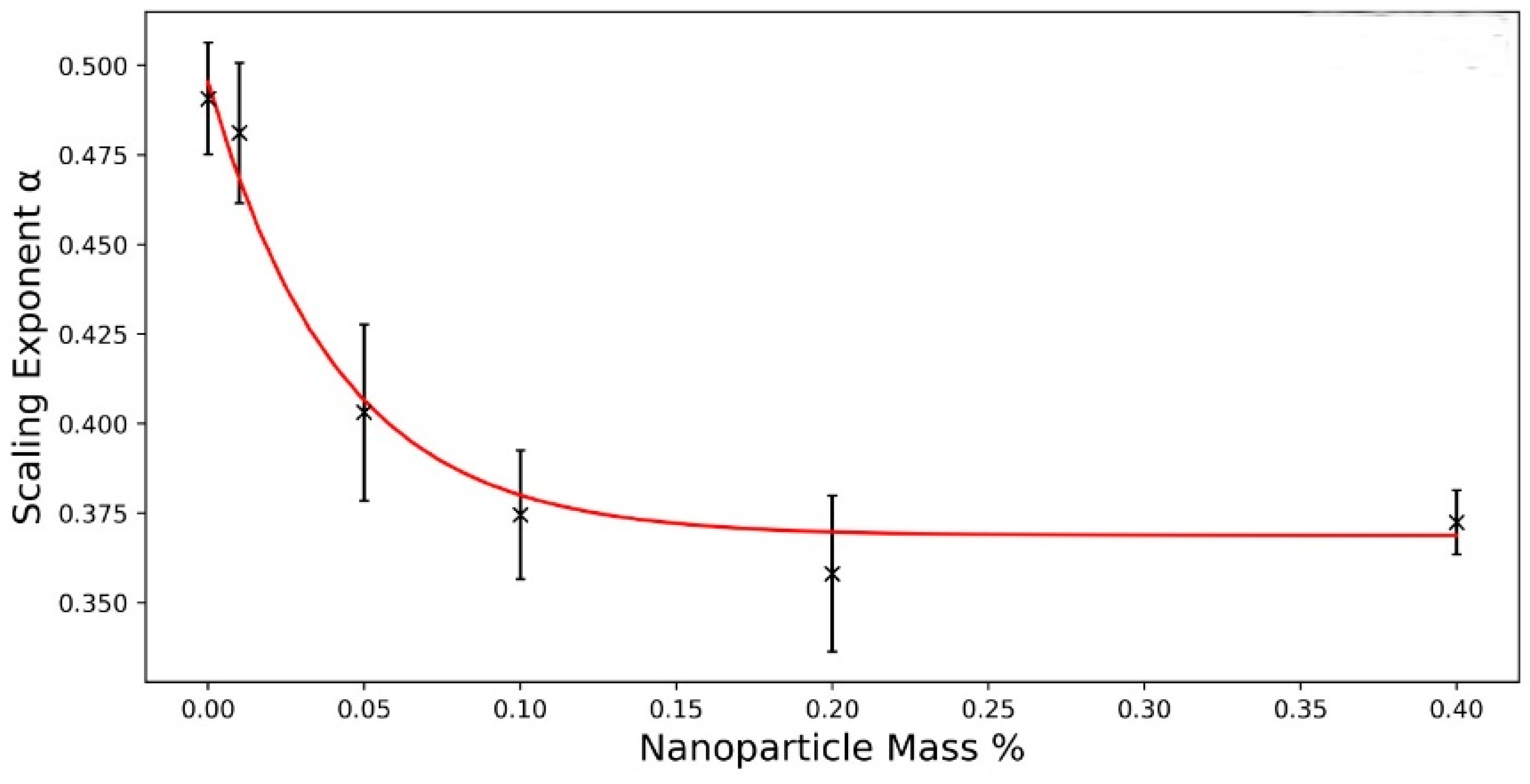
3.1. Variation of Mass Concentration at a Constant Particle Size
With this, we can proceed to discuss the annihilation exponents as a function of nanoparticle mass concentration at constant particle size of 280 nm, which is close to the middle of the investigated size range. The results are shown in Figure 7, with the red curve being a guide to the eye.
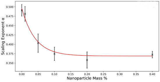
Figure 7.
Scaling exponent α as a function of nanoparticle mass concentration at a constant particle size of 280 nm.
At first, one can notice that for the neat liquid crystal, it is found within the limits of error that α = 0.49 ± 0.02; thus, α = 1/2, as expected from theoretical predictions and simulations [20,21,22,23,24] and confirmed by a range of experiments [6,7,8,31]. For increasing mass concentrations, the annihilation exponent decreases before saturating at approximately α = 0.37, which is clearly smaller than α = 1/2.
3.2. Variation of Particle Size at a Constant Particle Concentration
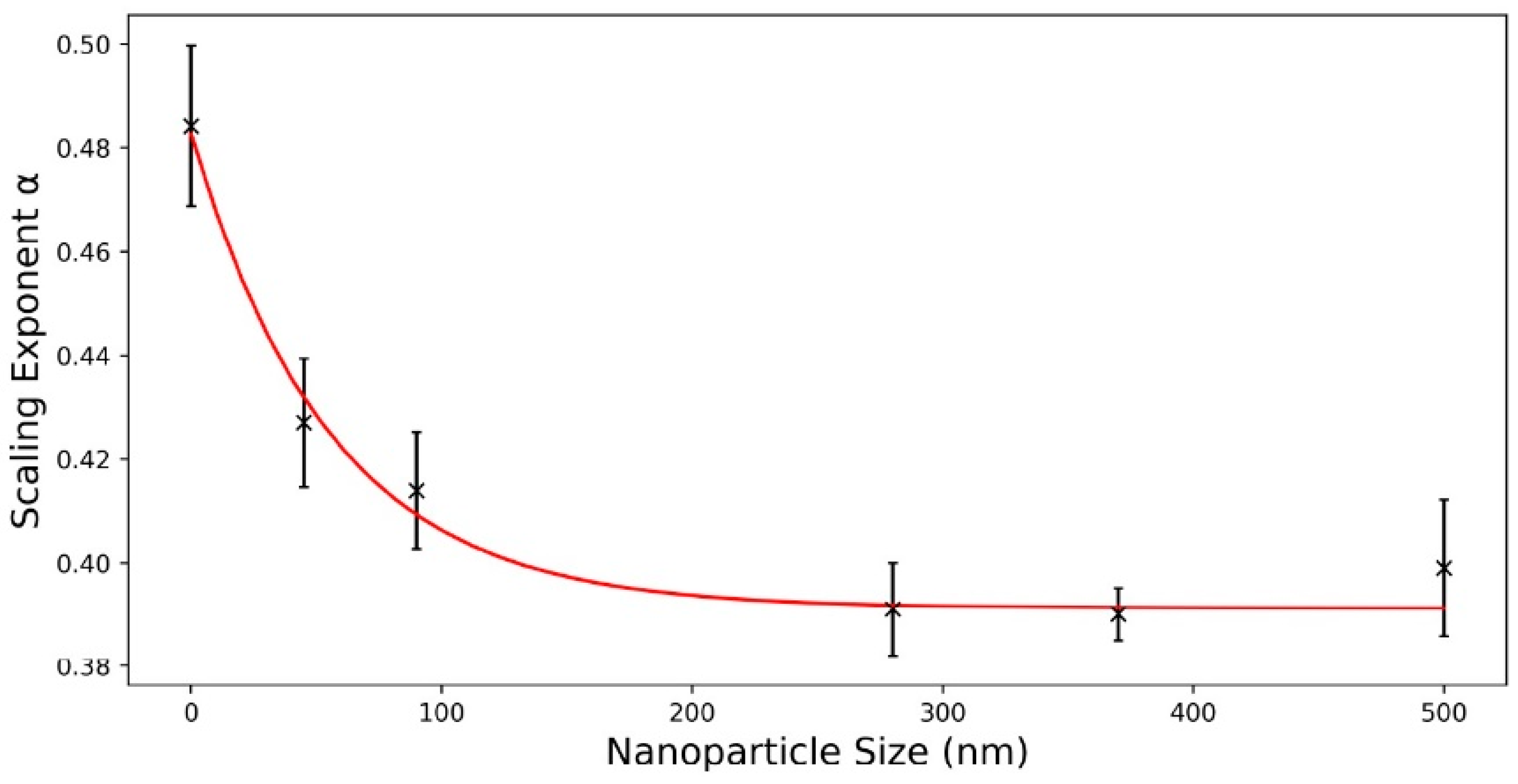
In the next series of experiments, the nanoparticle concentration was kept constant at 0.0002% and the particle size was varied between 45 nm and 500 nm, thus also varying the mass concentration (Figure 8).
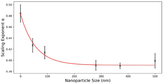
Figure 8.
Scaling exponent α for variations in particle size at a constant nanoparticle concentration of 0.0002%.
Within the limits of error, the neat liquid crystal shows a value of the annihilation exponent near 1/2, α = 0.483 ± 0.007, as expected. Again, the for the particle-laden systems, the annihilation exponent decreases, approaching a value of approximately α = 0.39, clearly lower than the predicted exponent.
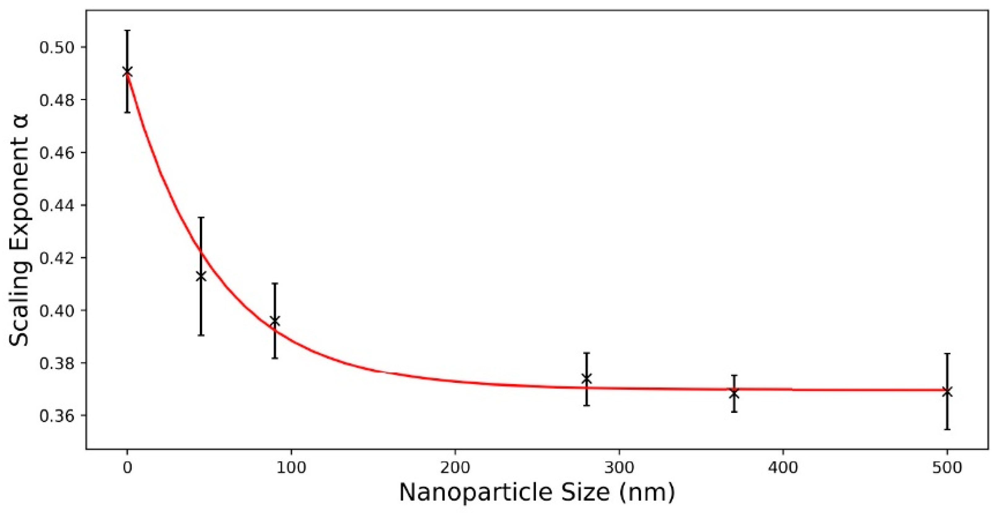
3.3. Variation of Nanoparticle Size at a Constant Mass Concentration
In the last experimental series, the nanoparticle size was varied between 45 and 500 nm at constant mass concentration of 0.1%, thus also varying the particle concentration. The results are shown in Figure 9.

Figure 9.
Defect annihilation scaling exponent α for variations in particle size at a constant mass concentration of 0.1%.
The exponent of the neat liquid crystal once again follows the predicted behavior, showing a value of α = 0.49 ± 0.02, which reproduces the predicted annihilation exponent of 1/2. The exponent decreases and saturates at a value of about α = 0.37.
The experiments in general suggest that neat liquid crystals, independent of their molecular species and of applied external conditions such as confining cell gap, applied electric field amplitude and frequency, or temperature, away from the vicinity of phase transitions, follow the predicted behavior based on theory and computer simulations. Nevertheless, nanoparticle-doped nematics appear to produce deviations from the accepted behavior, not with respect to the number density of defects observed when the nanoparticle size or concentration is varied, but rather with respect to the fundamental dynamics of defect annihilation, changing respective scaling exponents.
A possible explanation could be the accumulation of particles at the defects as the time to annihilation proceeds. It is known that nanoparticles accumulate within defect regions and at interfaces. Even though the particles do not appear to be acting as defect nucleation centers, they can be collected within the defect region while the defect moves through the liquid crystal–nanoparticle dispersion and also through diffusion and attractive forces. This can vary the defect velocity, as discussed below in relation to Figure 10, and thus change the drag force Fdrag (Equation (2)) with time. A number of factors would play into this scenario: (i) particle concentration, because more particles would be accumulated for higher concentrations within the same time, and (ii) particle size, because the larger the particle, the smaller the velocity caused by a constant drag. The velocity v (Equation (3)) would then become a function of time t, parametrized via particle concentration and particle size, which would change the obtained scaling exponent in Equation (6). It is justified to assume that there is a certain maximum number of particles of a given size which a defect can accommodate, explaining the saturation of the exponent α for increasing particle concentration, size, and thus overall mass. It would be of interest to verify such behavior through computer simulations.
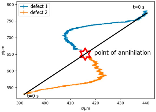
Figure 10.
S-shaped trajectory of two defects approaching the point of annihilation. Particle size is 280 nm at a mass concentration of 0.1%.
It is known based on theory and simulations [38,39] that attracting defects during the annihilation approach often travel in an S-shaped trajectory. A similar behavior is also observed in the experiments presented here, with an exemplary trajectory shown in Figure 10, which was determined via the same machine learning algorithm as outlined above. This shows that, ideally, machine learning in the future will facilitate investigation of this phenomenon in detail and provide insight into the fundamental mechanism of this type of dynamic behavior.
However, it is also known from experiments and simulations [32] of undoped liquid crystals that in general, the s = +1 defect has a speed about twice that of the s = −1 defect, v(+1) = 2v(−1), which is attributed to backflow effects [32,40]. The obtained data in Figure 10, on the other hand, suggest very equal speeds for both defects of opposite sign, indicating a reduction of v(+1) compared to a pure liquid crystal without nanoparticles. Possibly, the addition of nanoparticles prevents or diminishes backflow effects and modifies the viscous drag force, thus causing deviations in the generally observed behavior during defect annihilation and its scaling compared to non-doped systems.
4. Conclusions
By training and optimizing an image recognition algorithm based on machine learning, we were able to investigate the defect annihilation dynamics for an ensemble of annihilation events of umbilic defects of strength s = ±1 in detail. While the defect density is not affected by the addition of nanoparticles of various sizes and concentrations, the annihilation exponent is clearly affected when compared to the neat nematic liquid crystal system. The undoped nematic follows the predicted scaling law of square root functionality with exponent α = 1/2, while the addition of nanoparticles decreases the exponent by approximately 25% to saturate at about α = 0.38 ± 0.01 for increasing particle size and increasing particle concentration. A qualitative explanation is proposed. The experimental behavior suggests that for dispersions, the scaling of topological defect annihilation might be altered, despite the fact that changes in external conditions, such as liquid crystal material, applied electric field amplitude or frequency, temperature, and confining cell gap have been shown to not affect the respective scaling law.
Furthermore, the S-shaped defect trajectories, which have been predicted theoretically and via simulations, were experimentally verified, which have been proposed theoretically and via simulation. Nevertheless, the previously observed speed anisotropy of defects of opposite sign, which is attributed to backflow effects, could not be observed in nanoparticle-doped systems. One possible explanation is that the dispersed nanoparticles diminish backflow, which might also be the reason for the modified annihilation scaling laws. It would be of fundamental interest to further investigate this issue theoretically or with computer simulations.
Author Contributions
Conceptualization, I.D.; initial methodology, J.R.; improved methodology, A.M., G.M.C., K.S., L.H.; investigation, K.S., L.H., A.M., G.M.C.; resources, I.D.; writing—original draft preparation, I.D.; review and editing, I.D. and K.S.; supervision, I.D. All authors have read and agreed to the published version of the manuscript.
Funding
This research received no external funding.
Data Availability Statement
The original contributions presented in this study are included in the article. Further inquiries can be directed to the corresponding author.
Conflicts of Interest
The authors declare no conflict of interest.
References
- Chuang, I.; Durrer, R.; Turok, N.; Yurke, B. Cosmology in the laboratory: Defect dynamics in liquid crystals. Science 1991, 251, 1336. [Google Scholar] [CrossRef]
- Orihara, H.; Ishibashi, Y. Dynamics of Disclinations in Twisted Nematics Quenched below the Clearing Point. J. Phys. Soc. Jpn. 1986, 55, 2151–2156. [Google Scholar] [CrossRef]
- Orihara, H.; Nagaya, T.; Ishibashi, Y. Collective Motion of an Assembly of Disclinations in the Non-Orthogonally Twisted Nematics Quenched below the Clearing Point. Phys. Soc. Jpn. 1987, 56, 3086–3091. [Google Scholar] [CrossRef]
- Chuang, I.; Turok, N.; Yurke, B. Late-time coarsening dynamics in a nematic liquid crystal. Phys. Rev. Lett. 1991, 66, 2472. [Google Scholar] [CrossRef]
- Chuang, I.; Yurke, B.; Pargellis, A.N.; Turok, N. Coarsening dynamics in uniaxial nematic liquid crystals. Phys. Rev. E 1993, 47, 3343. [Google Scholar] [CrossRef]
- Pargellis, A.N.; Turok, N.; Yurke, B. Monopole-antimonopole annihilation in a nematic liquid crystal. Phys. Rev. Lett. 1991, 67, 1570. [Google Scholar] [CrossRef] [PubMed]
- Nagaya, T.; Hotta, H.; Orihara, H.; Ishibashi, Y. Observation of Annihilation Process of Disclinations Emerging from Bubble Domains. J. Phys. Soc. Jpn. 1991, 60, 1572–1578. [Google Scholar] [CrossRef]
- Nagaya, T.; Hotta, H.; Orihara, H.; Ishibashi, Y. Experimental Study of the Coarsening Dynamics of +1 and -1 Disclinations. J. Phys. Soc. Jpn. 1992, 61, 3511–3517. [Google Scholar] [CrossRef]
- Dierking, I.; Archer, P. Imaging liquid crystal defects. RSC Adv. 2013, 3, 26433. [Google Scholar] [CrossRef]
- Hindmarsh, M.B.; Kibble, T.W.B. Cosmic strings. Rep. Prog. Phys. 1995, 58, 411. [Google Scholar] [CrossRef]
- Zurek, W.H. Cosmological experiments in superfluid helium? Nature 1985, 317, 505–508. [Google Scholar] [CrossRef]
- Zurek, W.H. Cosmological experiments in condensed matter system. Phys. Rep. 1996, 276, 177–221. [Google Scholar] [CrossRef]
- Shankar, S.; Souslov, A.; Bowick, M.J.; Marchetti, M.C.; Vitelli, V. Topological active matter. Nat. Rev. Phys. 2022, 4, 380–398. [Google Scholar] [CrossRef]
- Ardaševa, A.; Doostmohammadi, A. Topological defects in biological matter. Nat. Rev. Phys. 2022, 4, 354–356. [Google Scholar] [CrossRef]
- Fardin, M.-A.; Ladoux, B. Living proof of effective defects. Nat. Phys. 2021, 17, 164–173. [Google Scholar] [CrossRef]
- Kralj, M.; Kralj, M.; Kralj, S. Topological Defects in Nematic Liquid Crystals: Laboratory of Fundamental Physics. Phys. Status Solidi A 2021, 218, 2000752. [Google Scholar] [CrossRef]
- Harth, K.; Stannarius, R. Topological Point Defects of Liquid Crystals in Quasi-Two-Dimensional Geometries. Front. Phys. 2020, 8, 112. [Google Scholar] [CrossRef]
- Shen, Y.; Dierking, I. Annihilation dynamics of topological defects induced by microparticles in nematic liquid crystals. Soft Matter 2019, 15, 8749–8757. [Google Scholar] [CrossRef] [PubMed]
- Imura, H.; Okano, K. Friction coefficient for a moving disinclination in a nematic liquid crystal. Phys. Lett. A 1973, 42, 403–404. [Google Scholar] [CrossRef]
- Toyoki, H. Pair annihilation of point like topological defects in the ordering process of quenched systems. Phys. Rev. A 1990, 42, 911. [Google Scholar] [CrossRef]
- Mondello, M.; Goldenfeld, N. Scaling and vortex dynamics after the quench of a system with a continuous symmetry. Phys. Rev. A 1990, 42, 5865. [Google Scholar] [CrossRef]
- Toyoki, H. Cell dynamics simulation for the phase ordering of nematic liquid crystals. Phys. Rev. E 1993, 47, 2558. [Google Scholar] [CrossRef] [PubMed]
- Jang, W.G.; Ginzburg, V.V.; Muzny, C.D.; Clark, N.A. Annihilation rate and scaling in a two-dimensional system of charged particles. Phys. Rev. E 1995, 51, 411. [Google Scholar] [CrossRef] [PubMed]
- Liu, C.; Muthukumar, M. Annihilation kinetics of liquid crystal defects. J. Chem. Phys. 1997, 106, 7822–7828. [Google Scholar] [CrossRef]
- Pargellis, A.N.; Finn, P.; Goodby, J.W.; Panizza, P.; Yurke, B.; Cladis, P.E. Defect dynamics and coarsening dynamics in smectic-C films. Phys. Rev. A 1992, 46, 7765. [Google Scholar] [CrossRef]
- Ding, D.-K.; Thomas, E.L. Structures of Point Integer Disclinations and Their Annihilation Behavior in Thermotropic Liquid Crystal Polyesters. Mol. Cryst. Liq. Cryst. 1994, 241, 103–117. [Google Scholar] [CrossRef]
- Wang, W.; Shiwaku, T.; Hashimoto, T. Experimental study of dynamics of topological defects in nematic polymer liquid crystals. J. Chem. Phys. 1998, 108, 1614–1625. [Google Scholar] [CrossRef]
- Rapini, A. Umbilics: Static properties and shear-induced displacements. J. Phys. 1973, 34, 629–633. [Google Scholar] [CrossRef]
- Saupe, A. Disclinations and Properties of the Director field in Nematic and Cholesteric Liquid Crystals. Mol. Cryst. Liq. Cryst. 1973, 21, 211–238. [Google Scholar] [CrossRef]
- Meyer, R.B. Point Disclinations at a Nematic-lsotropic Liquid Interface. Mol. Cryst. Liq. Cryst. 1972, 16, 355–369. [Google Scholar] [CrossRef]
- Dierking, I.; Marshall, O.; Wright, J.; Bulleid, N. Annihilation dynamics of umbilical defects in nematic liquid crystals under applied electric fields. Phys. Rev. E 2005, 71, 061709. [Google Scholar] [CrossRef]
- Dierking, I.; Ravnik, M.; Lark, E.; Healey, J.; Alexander, G.P.; Yeomans, J.M. Anisotropy in the annihilation dynamics of umbilic defects in nematic liquid crystals. Phys. Rev. E 2012, 85, 021703. [Google Scholar] [CrossRef] [PubMed]
- Beigmohammadi, M.; Sadigh, M.K.; Poursamad, J. Dielectric anisotropy changes in MBBA liquid crystal doped with barium titanate by a new method. Sci. Rep. 2024, 14, 5756. [Google Scholar] [CrossRef] [PubMed]
- Nelson, J.; Solawetz, J. Yolov5 is Here. 2020. Available online: https://blog.roboflow.com/yolov5-is-here/ (accessed on 5 January 2025).
- Redmon, J.; Divvala, S.; Girshick, R.; Farhadi, A. You only look once: Unified, realtime object detection. arXiv 2015, arXiv:1506.02640. [Google Scholar]
- Patel, M. Detailed Information on Different Versions of YOLO. Available online: https://towardsai.net/ (accessed on 5 January 2025).
- Wojke, N.; Bewley, A.; Paulus, D. Simple online and real-time tracking with a deep association metric. In Proceedings of the 2017 IEEE International Conference on Image Processing (ICIP), Beijing, China, 17–20 September 2017. [Google Scholar] [CrossRef]
- Missaoui, A.; Harth, K.; Salamon, P.; Stannarius, R. Annihilation of point defect pairs in freely suspended liquid-crystal films. Phys Rev Res. 2020, 2, 013080. [Google Scholar] [CrossRef]
- Tang, X.; Selinger, J.V. Annihilation trajectory of defects in smectic-C films. Phys. Rev. E 2020, 102, 012702. [Google Scholar] [CrossRef] [PubMed]
- Missaoui, A.; Lacaze, E.; Eremin, A.; Stannarius, R. Observation of Backflow during the Annihilation of Topological Defects in Freely Suspended Smectic Films. Crystals 2021, 11, 430. [Google Scholar] [CrossRef]


Disclaimer/Publisher’s Note: The statements, opinions and data contained in all publications are solely those of the individual author(s) and contributor(s) and not of MDPI and/or the editor(s). MDPI and/or the editor(s) disclaim responsibility for any injury to people or property resulting from any ideas, methods, instructions or products referred to in the content. |
© 2025 by the authors. Licensee MDPI, Basel, Switzerland. This article is an open access article distributed under the terms and conditions of the Creative Commons Attribution (CC BY) license (https://creativecommons.org/licenses/by/4.0/).