Abstract
In this paper, GH4079 alloy was thermally compressed under processing conditions of 1025 °C–1200 °C and 0.001 s−1–1 s−1. This article established the strain compensation Arrhenius constitutive equation, the improved Johnson–Cook constitutive equation, and the strain compensation Arrhenius constitutive model based on phase transition temperature segmentation and calculated the correlation coefficient (R) and local relative error (AARE) to verify the accuracy of the model, respectively. Finally, a certain microstructural analysis was combined. It can be concluded that the rheological stress of alloy GH4079 gradually decreases with the increase in temperature and strain rate. The AARE values of these three models are 21.09%, 20.47%, and 10.62%, respectively. The strain compensation Arrhenius model based on phase transition temperature segments can better describe the thermal deformation behavior of GH4079. By integrating this model, appropriate processing conditions can be selected to regulate the microstructural organization and achieve optimization during the practical application of the alloy.
1. Introduction
High-temperature alloys, or strong thermal alloys, have service temperatures above 600 °C. They can withstand large, complex stresses, have surface stability, and are highly alloyed nickel-based metal materials [1]. Because of their excellent mechanical strength, resistance to high-temperature creep, surface stability, and oxidation and corrosion resistance, they are extensively utilized in the aerospace industry. They are a crucial raw material for manufacturing aviation turbine engines [2]. GH4079 alloy (GH742Y) is based on GH4742 with increased V for strengthening. The alloy has higher Al, Ti, and Nb contents, which allows the formation of more Ni3 (AlTiNb) precipitation-reinforced phases compared to GH4742. This makes it an excellent raw material for aero-engine turbine disks and other parts, effectively enhancing the performance and extending the service life of the parts. The alloying elements have a significant impact on the properties of the alloy [3]. Compared to commercial alloys such as Waspalloy and RR1000, GH4079 contains a higher amount of Nb element, which provides greater strength and heat resistance, enabling it to operate stably at 800 °C for extended periods [4]. Therefore, this alloy shows promising prospects for development [2,5,6]. However, the deformation resistance of this alloy is relatively high and is sensitive to the thermal processing conditions, which poses significant challenges for the later forging deformation of the GH4079 high-temperature alloy. During the forging process of the GH4079 high-temperature alloy, if parameters are improperly selected, microstructural issues such as porosity and cracks may easily occur during deformation, affecting the alloy’s strength, hardness, and other properties. Consequently, it is crucial to investigate the hot deformation behavior of the GH4079 alloys for practical production. In thermal deformation experiments, the plastic deformation process of alloys is often studied through rheological behavior. The constitutive models can predict the thermal deformation capacity of materials under different conditions, facilitating the understanding of the organizational deformation laws of materials, which is one of the important methods for optimizing material processing design.
Materials undergo intricate microstructural changes as a result of varying deformation conditions, which play a critical role in determining the materials’ resistance to deformation and significantly influence macroscopic plastic deformation. The constitutive model is an expression that quantifies the relationship between rheological stress and deformation parameters, capable of quantitatively describing thermal deformation behavior. Among them, three typical constitutive models are widely applied, namely the Arrhenius [7], Johnson–Cook (JC) [8], and Fields–Backofen (FB) models [9]. Constructing the Arrhenius constitutive model is an effective method for studying the plastic flow behavior of various alloys such as aluminum, nickel-based alloys, and magnesium alloys. By applying this model, it is possible to effectively predict the microstructural changes of materials under different conditions. However, the predictive effect of the recently developed stress compensation hyperbolic sine Arrhenius model is more accurate [10,11]. The J-C constitutive model is typically used for metals that undergo significant deformations at high strain rates and temperatures, which offers the benefits of requiring fewer computational parameters, less experimentation, and simpler computational methods [12,13,14]. To date, researchers have evaluated and compared the accuracy of various models for predicting flow stresses in different materials [15]. Cai [16] et al. established the strain-compensated Arrhenius, J-C, and F-B models and their improved models using data obtained for 33Cr23NiMn3N heat-resistant steel under different conditions. Among them, the Arrhenius constitutive model with strain compensation predicts the best results. He [17] et al. established the J-C model, the improved J-C model, and the strain-compensated Arrhenius constitutive model for 20CrMo alloy steel over a wide temperature range. Through the analysis of stress values and predicted outcomes from comparative experiments, except for the J-C model, the other two models demonstrate relatively high accuracy. Consequently, this study conducts thermal compression experiments on the GH4079 alloy, an improved J-C model, a strain-compensated Arrhenius constitutive model, and a strain-compensated Arrhenius constitutive model based on phase–transition–temperature segmentation, allowing for a detailed analysis and comparison of the accuracy and effectiveness of these models.
2. Experimental Materials and Methods
The GH4079 alloy, composed of high-purity constituent elements (mass fraction greater than 99.9%), has its chemical composition shown in Table 1. The alloy is repeatedly melted in a vacuum arc furnace to ensure the uniformity of the alloy composition before forging. It is then subjected to standard heat treatment, with the basic process occurring at 1140 °C (8 h AC) (air cooling) and 850 °C (6 h AC + 16 h AC). Table 1 presents the quality percentage of the alloy. The wire-cutting process involved cutting the original forging alloys into cylindrical specimens with a diameter of 8 mm and a height of 12 mm. The Gleeble-3800 thermal compression simulation testing machine was used for the hot compression simulation experiments, as illustrated in Figure 1a: The simulation of the GH4079 alloy was the first to heat at a rate of 10 °C/s, gradually warming to 1200 °C. The mixture was maintained at this temperature for 5 to 10 min before cooling at a rate of 10 degrees Celsius per second and gradually reaching the temperature required for the thermal deformation process. After the internal temperature of the specimen reached a predetermined value, the temperature (1025 °C~1200 °C) and strain rate (0.001 s−1~1 s−1) were set for compression. The experiment was continuously conducted under the protective atmosphere of argon gas, and loading was stopped once the equivalent true strain reached the predetermined value. Subsequently, the thermally compressed sample was water-quenched to room temperature to preserve the microstructural state after thermal deformation. The characterization and analysis of the GH4079 alloy were conducted using Electron Backscatter Diffraction (EBSD) and Transmission Electron Microscopy (TEM). For the EBSD analysis, the sample was first polished with sandpaper and then electropolished for 30 s using a 10% HClO4 alcohol solution with a polishing voltage of 25 V. In this paper, the average nuclear orientation difference map (KAM) was obtained by EBSD processing to analyze the microstructure. By analyzing the KAM, one can qualitatively analyze the grain deformation, dislocation density distribution, and energy storage level [18]. For the TEM analysis, the deformed sample was ground to a thickness of 0.05 mm using sandpaper and then subjected to dual-jet electro-thinning, with the solution ratio as mentioned above. Before the hot compression simulation experiments, the original structure was characterized to ensure that it was relatively uniform, as shown in Figure 1b. The original structure consisted of dislocation-free, equiaxial crystals.

Table 1.
Composition of the GH4079 alloy.
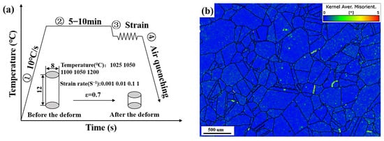
Figure 1.
(a) Flow chart of GH4079 alloy thermal compression simulation experiment; (b) KAM diagram of original structure before thermal compression simulation experiment.
3. Results and Discussion
3.1. Rheological Behavior Analysis of GH4079 Alloy
The magnitude of the flow stress depends on the interaction between work hardening (WH) and dynamic softening (dynamic recovery—DRV; dynamic recrystallization—DRX) [19]. The competition between softening behaviors and work hardening is interrelated. Typically, high-temperature alloys exhibit dynamic recrystallization-type features and dynamic restitution-type features during hot deformation [20]. As stress intensifies, the rheological stress surges sharply. Yet, once it reaches the peak stress (σp), the rheological stress begins to diminish with further increases in deformation. Finally, as the deformation process continues, the rheological stress gradually stabilizes, a state referred to as steady-state stress (σss). The latter shows that under the high-temperature conditions after the rheological stress reaches σp, there is no stress reduction, but the steady-state rheology with σp continues to be maintained. Figure 2 illustrates the σss and σp of the GH4079 alloy under specific conditions: an engineering strain of 0.7, a deformation temperature range of 1025 °C to 1200 °C, and a strain rate from 0.001 s⁻1 to 1 s⁻1. Maintaining a constant strain rate reveals a noteworthy trend: as temperature rises, both the steady-state and peak stresses significantly decline. This effect is particularly pronounced within the phase transition temperature range, where the reduction in peak and steady-state stresses occurs more steeply as temperatures increase. Understanding this relationship is crucial for optimizing material performance under varying thermal conditions. At high-temperature conditions, the thermal activation effect is significant, increasing the activity of atoms, thereby activating slip systems and facilitating dislocation slip. This movement reduces the accumulation of dislocations, resulting in a reduction in the alloy’s deformation resistance [21]. Moreover, elevated temperatures significantly amplify the dynamic softening effect. At high temperatures, the rheological stress rapidly peaks, aligning closely with the steady-state stress. As the strain rate rises, dislocations proliferate within the grains more rapidly, and the interaction among dislocations becomes stronger. This heightened interplay among dislocations suppresses dynamic softening, resulting in an increased flow stress.
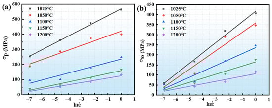
Figure 2.
(a) Peak stress and (b) steady-state stress of GH4079 alloy in different strain rate conditions.
3.2. The Arrhenius Model of Strain Compensation
The Arrhenius constitutive relationship is a phenomenological model [22] used to establish the relationship between material parameters and variations in flow stress. The expression is as follows:
where is the strain rate (s−1); α is the stress level parameter (MPa−1); σ is the flow stress (MPa); Z denotes the Zener-Hollomon parameter; R represents the universal gas constant. R = 8.314462618 J·mol−1·K−1, Q represents the activation energy required for thermal deformation (kJ/mol), T is the deformation temperature (K), and n1, n, β, α, and A are material constants, where α = β/n1. Additionally, the effect of strain during the process cannot be ignored. To enhance the precision of the parameters, we introduced strain as a variable in the study of the Arrhenius constitutive model with strain compensation. This article will take the condition of a strain of 0.3 as an example to demonstrate the calculation process, which is as follows: First, Formula (3) was substituted into (2), and, simultaneously, on both sides of the natural logarithmic function, Formula (4) can be obtained:
To facilitate subsequent calculations, Equation (4) is organized as follows:
where A1 and A2 are also material constants. The stresses under different temperature and strain rate conditions, with a strain variable of 0.3, are substituted into (5) and (6), and the scatter plots on and are linearly fitted, as illustrated in Figure 3. The values of 1/n1 and 1/β can be obtained from their slopes. The value of α for a strain of 0.3 is calculated by averaging these slopes; . According to Equation (7), n is the average value of the slope of the . The stress values in different conditions are substituted into (7) and then the value of n under each condition is obtained by linear fitting, as shown in Figure 3c. The average value of n under the condition of a strain of 0.3 is found to be 3.6533. From Equation (7), the following graphs were obtained:
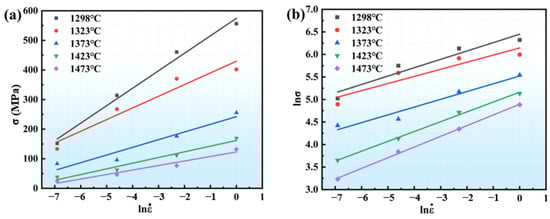
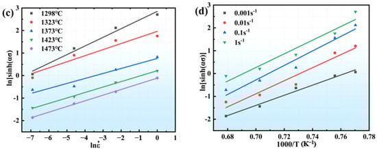
Figure 3.
Linear fit under different conditions: (a) ; (b) ; (c) ; (d) .
Accordingly, by plotting the curve of ln[sinh(ασ)] − 1000/T in different deformation conditions, the mean value of curve m is 28.1003. Under the condition of a strain of 0.3, by substituting n, m, and R into Equation (8), at a strain of 0.3, the Q value reaches 853.5214 kJ/mol. From Equations (1)–(3), the following is obtained:
Taking the natural logarithms of both sides of Equation (9) simultaneously, one obtains Equation (10):
The curve relating ln[sinh(ασ)] to lnZ effectively illustrates key parameters, where the slope indicates the value of n and the intercept signifies lnA. Using Equation (1), we can calculate the value of Z. As shown in Figure 4, the fitting curves for various parameters are compelling. The n value is 3.5 at a strain of 0.3, and the line is 70.5340.
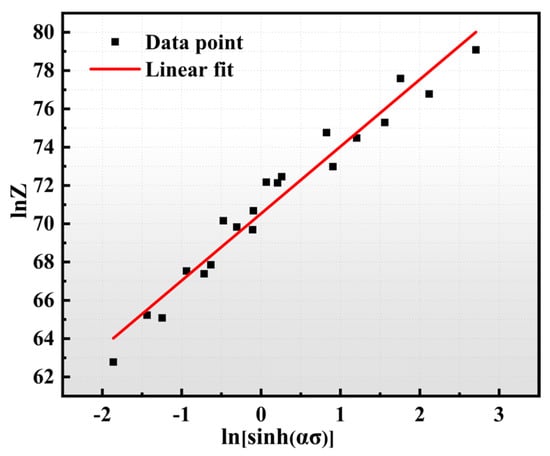
Figure 4.
ln[sinh(ασ)]-lnZ fit relationship.
As rheological stress varies with strain, the above calculation procedure selects a single strain variable for the derivation of the rheological stress. This ignores the effect of strain variables. The strain-compensated Arrhenius equation introduces the parameter of the strain variable and expresses individual material constants (α, n, lnA, and Q) in the constitutive equations as polynomial functions containing strain variables. For this study, strain variables ranging from 0.05~1 were selected for fitting, with a strain change gradient of 0.05, and a total of 20 sets of deformations were used. Through the polynomial fitting analysis, the error is minimized when applying the eighth-order polynomial to the material constants, and the fitting curve is shown in Figure 5. The polynomial function formula is shown as Equation (11), and the coefficients of the fitted polynomials are shown in Table 2.
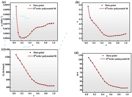
Figure 5.
Strain-compensated Arrhenius eigenstructure model with different parameter polynomial fits for (a) α-ε, (b) n-ε, (c) Q-ε, and (d) lnA-ε.
Table 2.
Fitting polynomial coefficients of Arrhenius constitutive model for strain compensation.
Substituting the fitted material constants into the expression of the hyperbolic sine function containing the Zener–Holloman parameter, the value of the rheological stress can be obtained under any deformation amount, as in Equation (12):
By substituting strain values ranging from 0.05 to 1 under various deformation conditions into Formula (12), we can derive the material constants for these strain levels. Figure 6 illustrates the comparison between the predicted and experimental values.
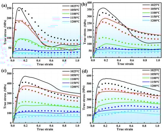
Figure 6.
A comparison of the predicted and experimental values of the strain-compensated Arrhenius eigenstructure model in different deformation conditions: (a) 0.001 s−1, 1050 °C~1200 °C; (b) 0.01 s−1, 1050 °C~1200 °C; (c) 0.1 s−1, 1050 °C~1200 °C; (d) 1 s−1, 1050 °C~1200 °C.
The predicted curve reveals that, when the phase transition temperature has not been reached, the predicted values are generally lower than the experimental values. Conversely, once the temperature exceeds the phase transition threshold, the predicted values tend to be higher than the experimental values. Therefore, the strain-compensated Arrhenius equation of the strain compensation based on the rheological stresses before and after the phase transition temperature is calculated. The parameters were fitted with an eighth-order polynomial. Figure 7 shows the fitting curves for different parameters, with coefficient values listed in Table 3. By substituting each strain into the Arrhenius equation based on strain compensation before and after the phase transition temperature, a comparison curve of predicted and experimental values was obtained, as shown in Figure 8.
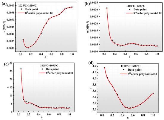
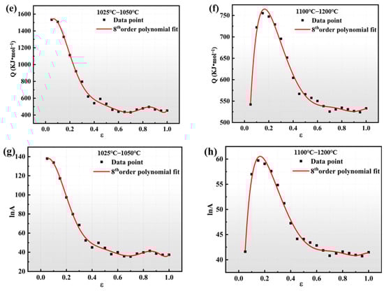
Figure 7.
Strain-compensated Arrhenius eigenmode coefficients based on polynomial fits before and after phase transition temperature for (a,b) α-ε, (c,d) n-ε, (e,f) Q-ε, (g,h) lnA-ε.
Table 3.
Fitted polynomial coefficients of the strain-compensated Arrhenius eigenmodes based on phase-change temperature segmentation.
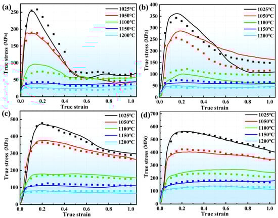
Figure 8.
A comparative analysis of the predicted and experimental values of the strain-compensated Arrhenius segmented principal model under different deformation conditions: (a) 0.001 s−1, 1050 °C~1200 °C; (b) 0.01 s−1, 1050 °C~1200 °C; (c) 0.1 s−1, 1050 °C~1200 °C; (d) 1 s−1, 1050 °C~1200 °C.
3.3. An Improved Johnson–Cook Model
The Johnson–Cook model is a strain relationship model for describing metallic materials at high temperatures and high strain rates. It was proposed by Johnson and Cook in 1983 and is now widely used due to its simplicity of form [23]. The expression is as follows:
where σ is the rheological stress (MPa), A is the yield stress corresponding to conditions, ε is the true strain, n is the strain hardening factor, C is the strain rate enhancement coefficient, is the dimensionless strain rate, is the strain rate (s−1), is the reference strain rate (s−1), T is the current temperature (K), is the melting temperature, is the reference temperature (T ≥ ), and m is the thermal softening coefficient.
However, the Johnson–Cook model falls short by ignoring the interplay between temperature and strain rate, which undermines its capacity to capture the comprehensive effects of all contributing factors. Conversely, the thermal deformation process in high-temperature alloys is deeply influenced by the intricate interaction of key elements such as strain rate, deformation temperature, and the degree of deformation, making it essential to consider these factors for a more accurate understanding. To address these shortcomings, an improved Johnson–Cook model has been proposed that incorporates these factors into account. The expression of the improved model is as follows [24]:
where A1, B1,…Bn, C1, λ1, and λ2 are material constants; , the rest of the covariates, and (13) are kept consistent. The improved Johnson–Cook model is used in this study, and two sets of reference points are selected before and after the phase transformation temperature: the reference temperature before the phase transformation temperature is 1050 °C (equivalent to 1323 K), and the reference strain rate is 0.01 s−1; the reference temperature after the phase transformation temperature is 1150 °C (equivalent to 1423 K), and the reference strain rate is 0.01 s−1. When the deformation temperature is the reference temperature and the strain rate is the reference strain rate, substituting it into Equation (14), then Equation (14) can be converted into (15):
The stress values before and after the phase transition for each deformation condition of 0.05~1 are taken and brought into (15), the scatter plots of ε and σ are plotted and polynomially fitted, and the error is minimized when the number of fits is 6, as shown in Figure 9. The coefficients before and after the phase transition point were determined through precise fitting, as illustrated in Table 4. When the deformation temperatures are the reference temperatures of 1323 K and 1423 K and the strain rates are 0.001 s−1~1 s−1, Equation (14) can be transformed into Equation (16):
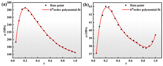
Figure 9.
σ versus ε for (a) reference temperature of 1050 °C, (b) reference temperature of 1150 °C.
Table 4.
Improved Johnson–Cook model parameters.
Converting Equation (16) into the form (17), that is, transforming it to the format presented in Equation (17), gives the following:
The stresses under different strain rate conditions are substituted into (17), the scatter plots are plotted before and after the phase transition relationship of −, respectively, and are then fitted linearly. The value of C1 is the slope of the curve, as shown in Figure 10, where the C1 values are 0.1975 and 0.3193, respectively. Then, Equation (14) can be converted into Equation (18):
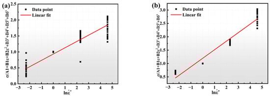
Figure 10.
Relationship diagram at (a) reference temperature of 1050 °C, and (b) reference temperature of 1150 °C.
Taking log ln for the left and right sides of (18), (18) can be converted into Equation (19):
When the strain variable is certain, the stress values are substituted for different temperatures and strains, and the fitted curve is plotted for the relationship , that is, one rate condition, where the strain corresponds to four sets of strain rate curves similarly. The fitted curves for the strain of 0.05~1 are plotted separately for the two reference point conditions, and the slopes of the curves correspond to the values of λ. Figure 11 displays the fitted curves for the two reference temperatures at a strain rate of 1 s−1. Concerning the fitted curves, the slopes, i.e., the values of λ of the curves, are −0.01043 and −0.0067, respectively. Since , the scatter plot is plotted and linearly fitted under different strain conditions, the slope of the curve is λ2, and the intercept of the curve is λ1. The modified Johnson–Cook model provides the intrinsic equations for the GH4079 alloy before and after the phase transition as follows:
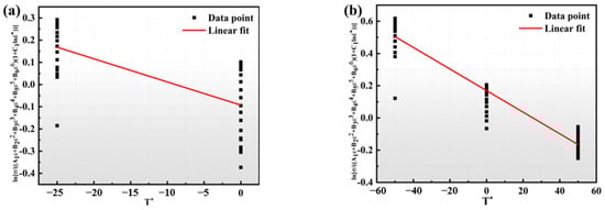
Figure 11.
Relationships between and (a) reference temperature of 1050 °C, (b) reference temperature of 1150 °C.
Different strain variables are substituted into the fitting equation and the accuracy of predicting stress by plotting scatter plots of predicted values and stress–strain curves is analyzed, as shown in Figure 12, and there are significant differences between the predicted and the experimental values for those conditions.
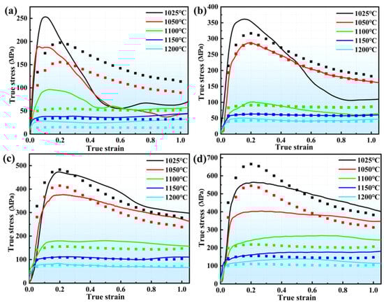
Figure 12.
A comparative analysis of the predicted and experimental values of the improved Johnson–Cook model in different deformation conditions: (a) 0.001 s−1, 1050 °C~1200 °C; (b) 0.01 s−1, 1050 °C~1200 °C; (c) 0.1 s−1, 1050 °C~1200 °C; (d) 1 s−1, 1050 °C~1200 °C.
3.4. Comparison of Strain-Compensated Arrhenius Eigenmodes, Segmented Strain-Compensated Arrhenius Eigenmodes, and Improved J-C Model
To further analyze and compare the accuracy of the three aforementioned models, we introduced the correlation coefficient (R) and average relative error (AARE) to determine the accuracy of each model. The formulas for these values are as follows:
where Ei and Pi denote the experimental and theoretical rheological stresses, respectively. Table 5 (A)(B)(C) shows the comparative analysis statistics of the relative errors of the GH4079 alloy in different conditions. After calculation, the relative error values of the strain-compensated Arrhenius model, the strain-compensated Arrhenius constitutive model based on segmentation before and after the phase transition temperature, and the improved Johnson–Cook model are 21.09%, 10.62%, and 20.47%, respectively. Figure 13 illustrates the correlation analysis between the predicted and experimental values of the rheological stresses for the three models. The correlation coefficients for three constitutive equations are as follows: the strain-compensated Arrhenius constitutive equation has a coefficient of 0.9449, the Arrhenius constitutive equation based on the segmentation of the phase transition temperature has a coefficient of 0.9787, and the improved Johnson–Cook constitutive equation has a coefficient of 0.9274. Among these three equations, the Arrhenius constitutive equation that incorporates the segmentation of the phase transition temperature demonstrates the highest prediction accuracy. It is particularly effective in predicting the rheological stress of the GH4079 alloy with greater accuracy.
Table 5.
A comparison of the AARE values under different deformation conditions for the three models.
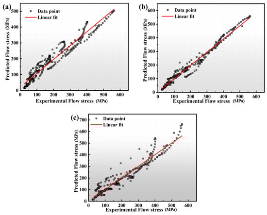
Figure 13.
The correlation coefficient of three constitutive models: (a) Strain-compensated Arrhenius model (b) Strain-compensated Arrhenius constitutive model based on segmentation before and after the phase transition temperature (c) Modified Johnson–Cook model.
3.5. Microstructure Analysis
During hot deformation of high-temperature alloys, the increase and decrease in flow stress is linked to dislocation changes [25]. During the prethermal deformation period, with increasing temperature and strain rate, the amount of distortion energy stored inside the grains increases rapidly, causing dislocation proliferation rapidly and accumulating at the grain boundary. The work-hardening effect is significant, leading to a rapid increase in rheological stress. As strain increases, the effects of dynamic recrystallization (DRX) and dynamic recovery (DRV) also become more pronounced [26]. With the enhancement in dynamic softening and the balance of work hardening, viscous stress rises slowly and eventually stabilizes after reaching its peak. At this time, DRV and DRX become the main mechanism; the macroscopic manifestation is the decrease in flow stress, and the microscopic manifestation is the annihilation of dislocation [27]. Hence, in this paper, the KAM (kernel-averaged orientation difference) map, obtained through EBSD post processing, was utilized for in-depth analysis of the recrystallization behavior of the high-temperature alloys under study [28]. The KAM is proportional to the dislocation density, and according to the KAM plot, the color gradually changes from red to blue, which indicates that the KAM value varies from large to small, and the low KAM indicates a low dislocation density [29,30]. Figure 14a~c represent the KAM plots at a strain rate of 0.01 s−1 and a temperature of 1050 °C~1150 °C, respectively, and Figure 14d~f represent the KAM plots at the deformation temperature of 1100 °C and a strain rate of 0.001 s−1~1 s−1, respectively. Through comparative analysis, under conditions of a low temperature and high strain rate, dislocations tend to accumulate easily, resulting in a relatively high density. The energy and time required to form the dynamic softening effect are insufficient, the number of recrystallized grains is relatively small, and the main concentration is at the original grain boundaries, leading to a relatively weak dynamic softening effect. Additionally, a significant number of dislocations are plugged, and their density increases, thus generating an obvious work-hardening phenomenon, and the macroscopic reaction is an increase in flow stress. In contrast, at high deformation temperatures and low strain rates, the activation energy increases, the motion of atoms being more active, promoting the rearrangement and disappearance of dislocations, resulting in a lower dislocation density in the alloy. Simultaneously, sufficient time allows for the growth of recrystallization nuclei, enhancing the dynamic softening effect. In addition, as shown in Figure 14b, there are obvious necklaces of recrystallized grains around the larger deformed grains, and dislocations are clustered at the grain boundaries, which gradually expands to the inside of the deformed grains. Additionally, there are almost no dislocations inside the newly formed recrystallized grains, which suggests that, during the process of dynamic recrystallization., it is necessary to absorb dislocations continuously to achieve the transformation of the subcrystalline grains into recrystallized grains from the subcrystalline grains [31].
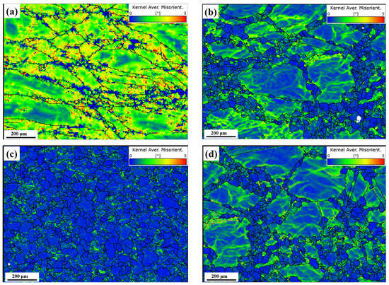
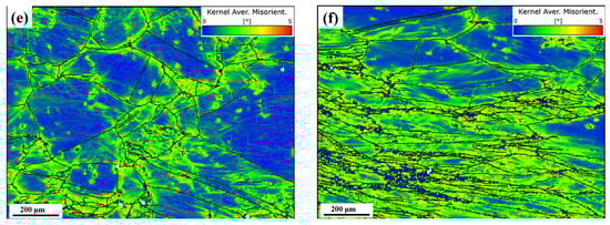
Figure 14.
KAM plots of the specimens after the deformation of the GH4079 alloy: (a–c) the strain rate is 0.01 s−1, the deformation temperature is 1050 °C~1150 °C; (d–f) the deformation temperature is 1100 °C; the strain rate is 0.001 s−1~1 s−1.
Figure 15 presents the TEM images taken at a temperature of 1050 °C with a strain rate of 0.01 s⁻1, and at 1100 °C with a strain rate of 1 s⁻1, respectively. Figure 15a shows that a significant number of reticulations or high-density entanglements are formed inside the alloy under low-temperature conditions, and Figure 15b shows relatively few dislocation interactions; the dislocation wall gradually forms, and obvious bowing out of grain boundaries can be observed, which is an obvious dynamic recrystallization phenomenon, indicating that the dislocations need to be absorbed continuously during the process [32,33], while Figure 15c shows many elongated deformed grains and surrounding high-density entangled dislocation structures. Furthermore, as demonstrated in Figure 15a, the precipitated phase is concentrated in the region with a dense dislocation distribution and interacts with it. This interaction suggests that the precipitated phase possesses a crucial role in the deformation process of the GH4079 alloy during the preheating deformation stage [34]. In summary, the thermal deformation process of the GH4079 alloy is closely related to changes in the dislocation configuration and the role of precipitates. The changes in the microstructure are consistent with the judgments made earlier, and by combining the Arrhenius-type constitutive equation based on the phase transition temperature segments, we can accurately predict the flow stress of the GH4079 alloy. This method allows us to anticipate shifts in microstructural organization, thereby significantly reducing the potential for cracking in real-world applications.
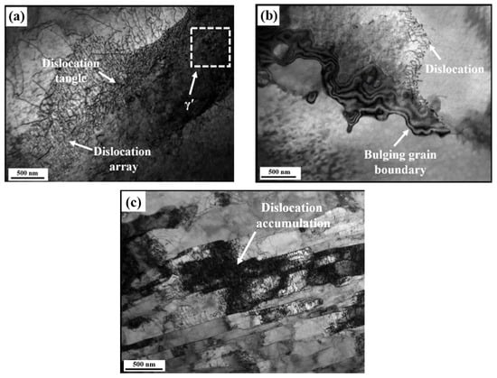
Figure 15.
TEM images of specimens of GH4079 alloy after deformation: (a) 1050 °C, 0.01 s−1; (b) 1100 °C, 0.01 s−1; (c) 1100 °C, 1 s−1.
4. Conclusions
- In the thermal deformation experiment of alloy GH4079, the value of the flow stress is directly proportional to the deformation temperature and inversely proportional to the strain rate.
- The rheological stresses of the GH4079 alloy were computed by applying the strain-compensated Arrhenius constitutive equation, the Arrhenius constitutive equation based on the segmentation of the phase transition temperature, and the improved Johnson–Cook constitutive equation. The correlation coefficients of the three models were 0.94449, 0.9787, and 0.9274, respectively, and the AARE values were 21.09%, 10.62%, and 20.47%, respectively. Combining these three models, the Arrhenius constitutive equation based on phase transition temperature segmentation has the highest accuracy.
- The alloy identified as GH4079 demonstrates a significantly higher dislocation density during the thermal deformation process at low temperatures and high strain rates, which directly impacts the macroscopic rheological stress. Furthermore, the presence of precipitated phases plays a crucial role in influencing the rheological behavior of the material. Therefore, by integrating the Arrhenius constitutive equation based on the segmentation of the phase transition temperature with a high precision to predict the microstructural evolution of the alloy under various conditions, we can avoid cracking issues in practical applications. This approach not only enhances the material’s performance but also ensures reliability in demanding environments.
Author Contributions
Conceptualization, W.Y. and J.H.; methodology, W.Y.; software, S.J.; validation, W.Y. and J.W.; formal analysis, W.Y.; investigation, J.H.; resources, W.Y.; data curation, W.Y.; writing—original draft preparation, W.Y.; writing—review and editing, J.H.; visualization, S.J.; supervision, J.H.; project administration, J.W.; funding acquisition, S.J. All authors have read and agreed to the published version of the manuscript.
Funding
This research received no external funding.
Data Availability Statement
The original contributions presented in this study are included in the article. Further inquiries can be directed to the corresponding author(s).
Conflicts of Interest
The authors declare that they have no known competing financial interests or personal relationships that could have appeared to influence the work reported in this paper.
References
- Liu, D.H.; Chai, H.R.; Yang, L.; Qiu, W.Q.; Guo, Z.H.; Wang, Z.L. Study on the dynamic recrystallization mechanisms of GH5188 superalloy during hot compression deformation. J. Alloys Compd. 2022, 895, 162565. [Google Scholar] [CrossRef]
- Miao, Q.; Ding, W.F.; Xu, J.H.; Cao, L.J.; Wang, H.C.; Yin, Z.; Dai, C.W.; Kuang, W.J. Creep feed grinding induced gradient microstructures in the superficial layer of turbine blade root of single crystal nickel-based superalloy. Int. J. Extreme Manuf. 2021, 3, 045102. [Google Scholar] [CrossRef]
- Cheng, Z.Y.; Zhao, Q.; Tao, M.J.; Du, J.J.; Huang, X.X.; Liu, C.J. Preparation of FeCoNi medium entropy al-loy from Fe3+-Co2+-Ni2+ solution system. Int. J. Min. Met. Mater. 2025, 32, 92–101. [Google Scholar] [CrossRef]
- Zhang, W.W.; Liu, X.G.; Lu, T.G.; Liu, Y.L.; Guo, Y.; Qin, H.Y.; Tian, Q. Microstructural evolution of GH4079 superalloy during hot deformation and heat treatment. J. Mater. Res. Technol. 2024, 33, 298–317. [Google Scholar] [CrossRef]
- Zhang, W.W.; Liu, X.A.; Du, Q.; Li, H.Z.; Qin, H.Y.; Tian, Q. Hot Deformation Behavior and Dynamic recrystallization mechanism transition of GH4742 Ni-Based superalloy under various deformation conditions. J. Mater. Eng. Perform. 2023, 32, 3253–3273. [Google Scholar] [CrossRef]
- Zhang, X.J.; Zhuo, G.; Zhang, H.Y.; Ma, X.; Gan, B.; Chen, L.J. Study of Processing Map of GH4079 Alloy Based on Different Instability Criteria. JOM 2024, 76, 3872–3887. [Google Scholar] [CrossRef]
- Sellars, C.M.; McTegart, W.J. On the mechanism of hot deformation. Acta Metall. 1966, 14, 1136–1138. [Google Scholar] [CrossRef]
- Johnson, G.R.; Cook, W.H. A constitutive model and data for metals subjected to large strains, high strain rates and high temperature. Eng. Fract. Mech. 1983, 21, 541–543. [Google Scholar]
- Fields, D.S.; Backofen, W.A. Determination of strain hardening characteristics by torsion testing. Proc. Am. Soc. Test Mater. 1957, 57, 1259–1272. [Google Scholar]
- Wang, H.; Qin, G.L.; Li, C.A. Modified Arrhenius constitutive model of 2219-O aluminum alloy based on hot compression with simulation verification. J. Mater. Res. Technol. 2022, 19, 3302–3320. [Google Scholar] [CrossRef]
- Harikrishna, K.; Bhowmik, A.; Davidson, M.J.; Kumar, R.; Anqi, A.E.; Rajhi, A.A.; Alamri, S.; Kumar, R. Evaluation of constitutive equations for modeling and characterization of microstructure during hot deformation of sintered Al-Zn-Mg alloy. J. Mater. Res. Technol. 2024, 28, 1523–1537. [Google Scholar] [CrossRef]
- Zhu, S.S.; Liu, J.; Deng, X. Modification of strain rate strengthening coefficient for Johnson-Cook constitutive model of Ti6Al4V alloy. Mater. Today Commun. 2021, 26, 102016. [Google Scholar] [CrossRef]
- Xie, G.L.; Yu, X.T.; Gao, Z.F.; Xue, W.L.; Zheng, L. The modified Johnson-Cook strain-stress constitutive model according to the deformation behaviors of a Ni-W-Co-C alloy. J. Mater. Res. Technol. 2022, 20, 1020–1027. [Google Scholar] [CrossRef]
- Jia, W.T.; Xu, S.; Le, Q.C.; Fu, L.; Ma, L.F.; Tang, Y. Modified Fields-Backofen model for constitutive behavior of as-cast AZ31B magnesium alloy during hot deformation. Mater. Des. 2018, 106, 120–132. [Google Scholar] [CrossRef]
- Shen, J.Y.; Hu, L.X.; Sun, Y.; Wan, Z.P.; Feng, X.Y.; Ning, Y.Q. A comparative study on artificial neural network, phenomenological-based constitutive and modified Fields-Backofen Models to predict flow stress in Ti-4Al-3V-2Mo-2Fe alloy. J. Mater. Eng. Perform. 2019, 28, 4302–4315. [Google Scholar] [CrossRef]
- Cai, Z.M.; Ji, H.C.; Pei, W.C.; Wang, B.Y.; Huang, X.M.; Li, Y.M. Constitutive equation and model validation for 33Cr23Ni8Mn3N heat-resistant steel during hot compression. Results Phys. 2019, 15, 102633. [Google Scholar] [CrossRef]
- He, A.; Xie, G.L.; Zhang, H.L.; Wang, X.T. A comparative study on Johnson-Cook, modified Johnson-Cook and Arrhenius-type constitutive models to predict the high-temperature flow stress in 20CrMo alloy steel. Mater. Des. 2013, 52, 677–685. [Google Scholar] [CrossRef]
- Song, Y.H.; Li, Y.G.; Li, H.Y.; Zhao, G.H.; Cai, Z.H.; Sun, M.X. Hot deformation and recrystallization behavior of a new nickel-base superalloy for ultra-supercritical applications. J. Mater. Res. Technol. 2022, 19, 4308–4324. [Google Scholar] [CrossRef]
- Li, Y.J.; Zhang, Y.; Chen, Z.Y.; Ji, Z.C.; Zhu, H.Y.; Sun, C.F.; Dong, W.P.; Li, X.; Sun, Y.; Yao, S. Hot deformation behavior and dynamic recrystallization of GH690 nickel-based superalloy. J. Alloys Compd. 2020, 847, 156507. [Google Scholar] [CrossRef]
- Wu, B.; Li, M.Q.; Ma, D.W. The flow behavior and constitutive equations in isothermal compression of 7050 aluminum alloy. Mater. Sci. Eng. A 2012, 542, 79–87. [Google Scholar] [CrossRef]
- Jia, D.; Sun, W.R.; Xu, D.S.; Yu, L.X.; Xin, X.; Zhang, W.H.; Qi, F. Abnormal dynamic recrystallization behavior of a nickel-based superalloy during hot deformation. J. Alloys Compd. 2019, 787, 196–205. [Google Scholar] [CrossRef]
- Huang, M.J.; Jiang, J.F.; Wang, Y.; Liu, Y.Z.; Zhang, Y.; Dong, J.; Tong, Z.Y. Unraveling hot deformation behavior and microstructure evolution, flow stress prediction of powder metallurgy BCC/B2 Al1.8CrCuFeNi2 HEA. J. Alloys Compd. 2024, 972, 172828. [Google Scholar] [CrossRef]
- Ashtiani, H.R.; Shahsavari, P. A comparative study on the phenomenological and artificial neural network models to predict hot deformation behavior of AlCuMgPb alloy. J. Alloys Compd. 2016, 687, 263–273. [Google Scholar] [CrossRef]
- Amitava, R.; Mohammad, A.; Satyabrata, D.; Rupa, D. Constitutive modeling for predicting high-temperature flow behavior in aluminum 5083 + 10 wt Pct SiCP composite. Metall. Mater. Trans. B 2019, 50, 1060–1076. [Google Scholar]
- Zhang, J.B.; Wu, C.J.; Peng, Y.Y.; Xia, X.C.; Li, J.A.; Ding, J.; Liu, C.; Chen, X.G.; Dong, J.; Liu, Y.C. Hot compression deformation behavior and processing maps of ATI 718Plus superalloy. J. Alloys Compd. 2020, 835, 155195. [Google Scholar] [CrossRef]
- Li, N.; Zhang, F.G.; Yang, Q.; Wu, Y.; Wang, M.L.; Liu, J.; Wang, L.; Chen, Z.; Wang, H.W. Microstructure and Mechanical Properties of In Situ TiB2/2024 Composites Fabricated by Powder Metallurgy. J. Mater. Eng. Perform. 2022, 31, 8775–8783. [Google Scholar] [CrossRef]
- Zhong, X.T.; Wang, L.; Huang, L.K.; Liu, F. Transition of dynamic recrystallization mechanism during hot deformation of Incoloy 028 alloy. J. Mater. Sci. Technol. 2020, 42, 241–253. [Google Scholar] [CrossRef]
- Lin, Y.C.; Wu, X.Y.; Chen, X.M.; Chen, J.; Wen, D.X.; Zhang, J.L.; Li, L.T. EBSD study of a hot deformed nickel-based superalloy. J. Alloys Compd. 2015, 640, 101–113. [Google Scholar] [CrossRef]
- Li, H.Y.; Feng, W.; Zhuang, W.H.; Hua, L. Microstructure analysis and segmented constitutive model for Ni-Cr-Co-based superalloy during hot deformation. Metals 2022, 12, 357. [Google Scholar] [CrossRef]
- Sun, B.; Zhang, T.B.; Song, L.; Zhang, L. Microstructural evolution and dynamic recrystallization of a nickel-based superalloy PM EP962NP during hot deformation at 1150 °C. J. Mater. Res. Technol. 2022, 18, 1436–1449. [Google Scholar] [CrossRef]
- Chen, X.M.; Lin, Y.C.; Wen, D.X.; Zhan, J.L.; He, M. Dynamic recrystallization behavior of a typical nickel-based superalloy during hot deformation. Mater. Des. 2014, 57, 568–577. [Google Scholar] [CrossRef]
- Mi, J.; Ma, D.Q.; Luan, S.Y.; Jin, P.P.; Chen, L.J.; Che, X.; Li, X.Q. The hot deformation behavior and microstructural evolution of as-cast Mg-2Zn-0.5Mn-0.2Ca-0.3Nd-0.7La alloy. J. Mater. Res. Technol. 2023, 22, 1533–1545. [Google Scholar] [CrossRef]
- Qin, D.H.; Wang, M.J.; Sun, C.Y.; Su, Z.X.; Qian, L.Y.; Sun, Z.H. Interaction between texture evolution and dynamic recrystallization of extruded AZ80 magnesium alloy during hot deformation. Mater. Sci. Eng. A 2020, 788, 139537. [Google Scholar] [CrossRef]
- Huang, K.; Marthinsen, K.; Zhao, Q.L.; Logé, R.E. The double-edge effect of second-phase particles on the recrystallization behavior and associated mechanical properties of metallic materials. Prog. Mater. Sci. 2018, 92, 284–359. [Google Scholar] [CrossRef]
Disclaimer/Publisher’s Note: The statements, opinions and data contained in all publications are solely those of the individual author(s) and contributor(s) and not of MDPI and/or the editor(s). MDPI and/or the editor(s) disclaim responsibility for any injury to people or property resulting from any ideas, methods, instructions or products referred to in the content. |
© 2025 by the authors. Licensee MDPI, Basel, Switzerland. This article is an open access article distributed under the terms and conditions of the Creative Commons Attribution (CC BY) license (https://creativecommons.org/licenses/by/4.0/).