
Wavy Ice Patterns as a Result of Morphological Instability of an Ice–Water Interface with Allowance for the Convective–Conductive Heat Transfer Mechanism


Abstract
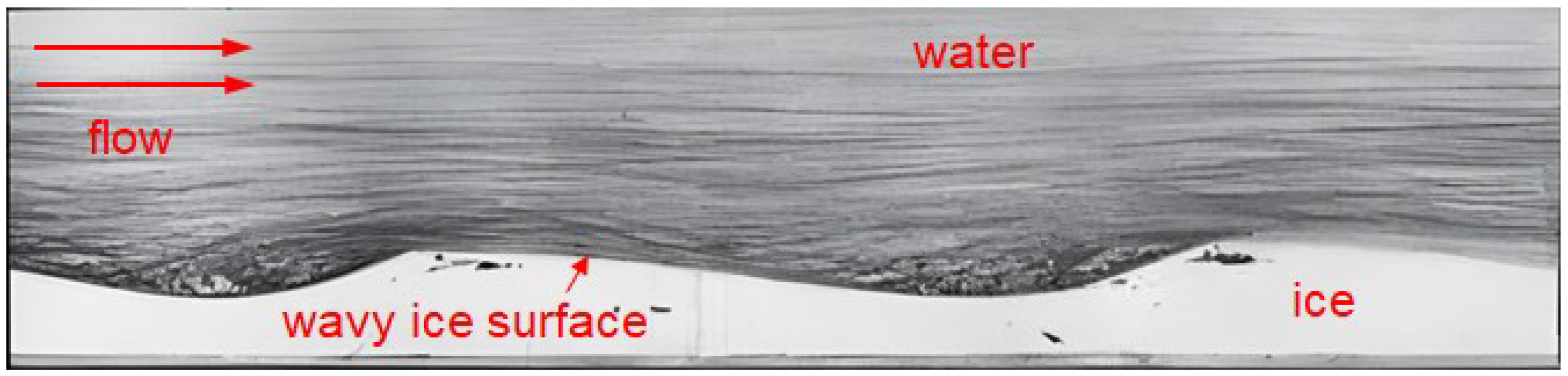
1. Introduction
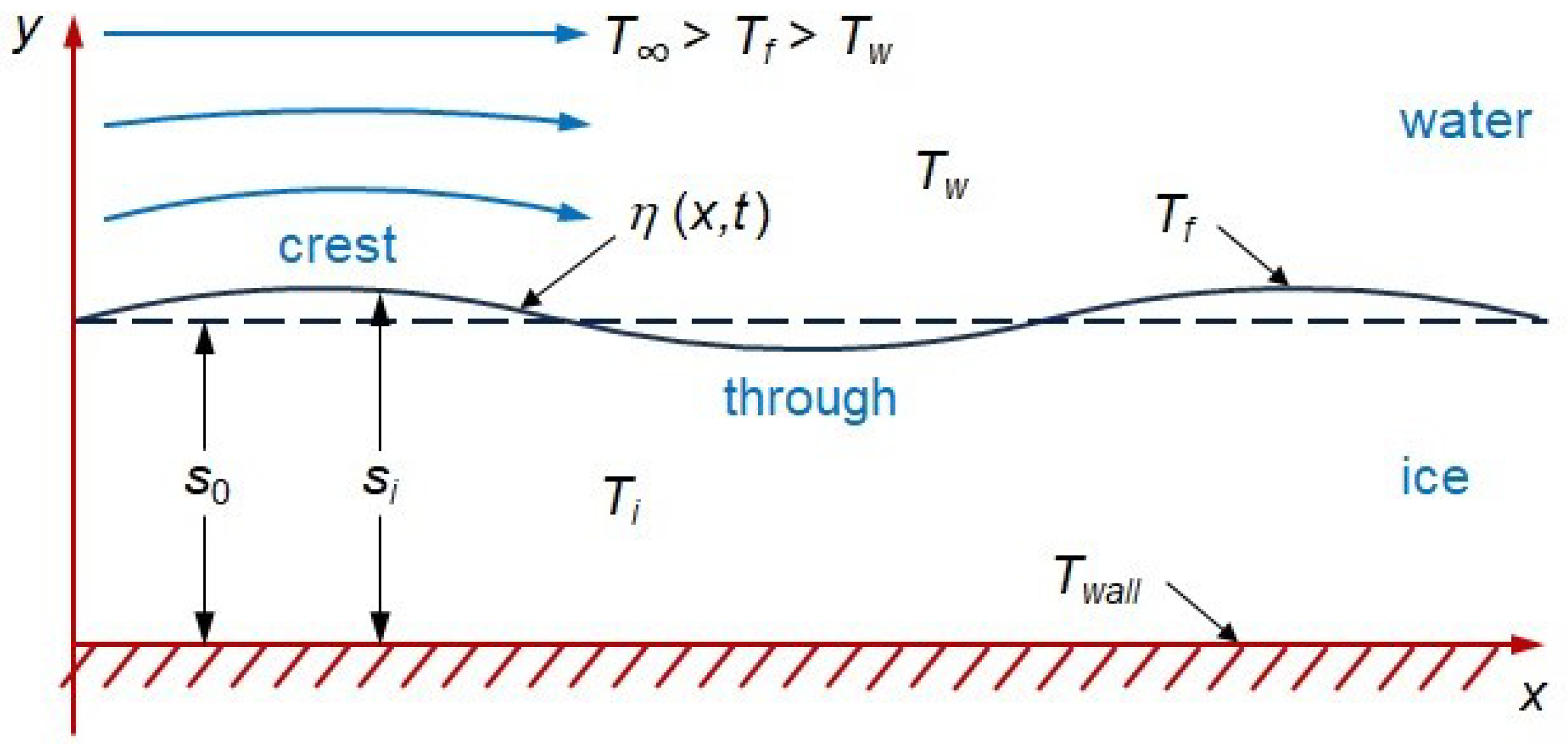
2. Morphological Stability
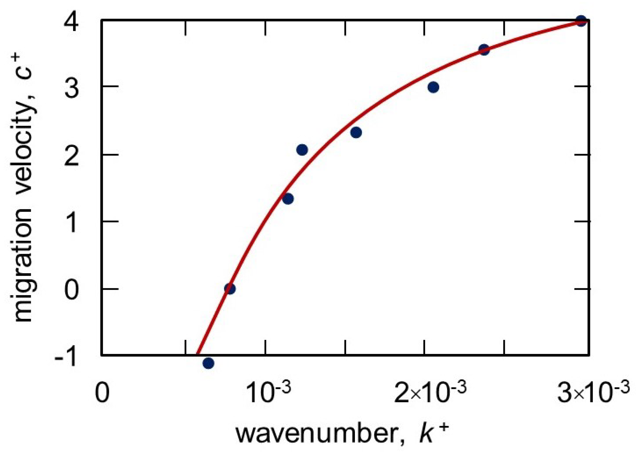
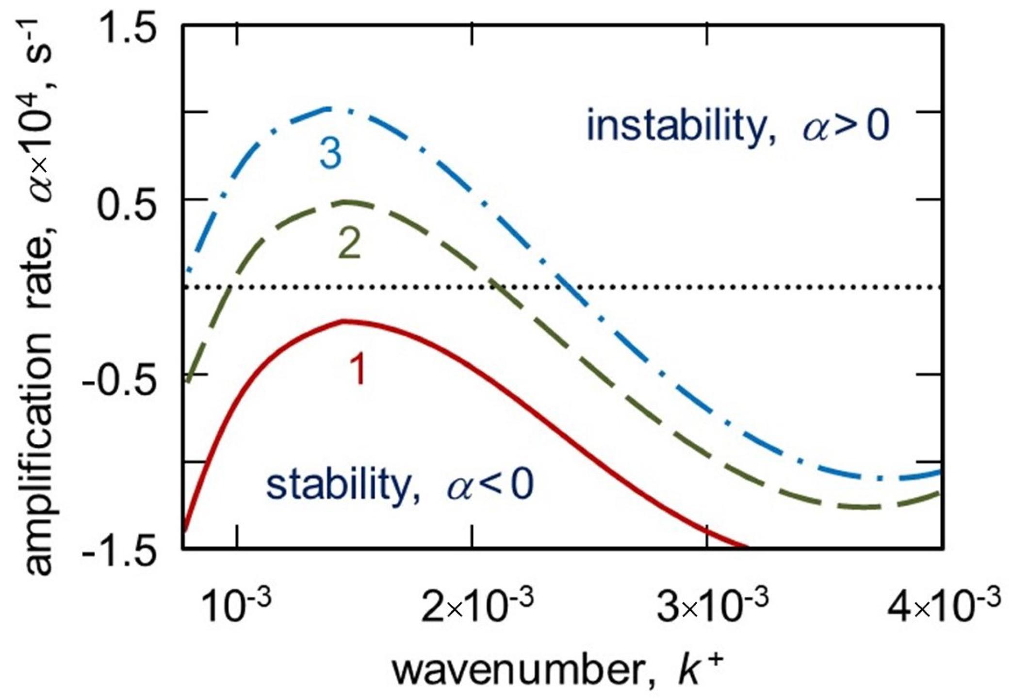
3. Results and Discussions
4. Conclusions
Author Contributions
Funding
Data Availability Statement
Conflicts of Interest
References
- Li, N.; Tuo, Y.C.; Deng, Y.; Li, J.; Liang, R.F.; An, R.D. Heat transfer at ice-water interface under conditions of low flow velocities. J. Hydrodyn. 2016, 28, 603–609. [Google Scholar] [CrossRef]
- Rafat, A.; Pour, H.K.; Spence, C.; Palmer, M.J.; MacLean, A. An analysis of ice growth and temperature dynamics in two Canadian subarctic lakes. Cold Reg. Sci. Technol. 2023, 210, 103808. [Google Scholar] [CrossRef]
- Alexandrov, D.V.; Netreba, A.V.; Malygin, A.P. Time-dependent crystallization in magma chambers and lava lakes cooled from above: The role of convection and kinetics on nonlinear dynamics of binary systems. Int. J. Heat Mass Trans. 2012, 55, 1189–1196. [Google Scholar] [CrossRef]
- Nizovtseva, I.G.; Starodumov, I.O.; Pavlyuk, E.V.; Ivanov, A.A. Mathematical modeling of binary compounds with the presence of a phase transition layer. Math. Methods Appl. Sci. 2021, 44, 12260–12270. [Google Scholar] [CrossRef]
- Notz, D.; Worster, M.G. In situ measurements of the evolution of young sea ice. J. Geophys. Res. Ocean. 2008, 113, C03001. [Google Scholar] [CrossRef]
- Stamou, A.C.; Radulovic, J.; Buick, J.M. Effect of stenosis growth on blood flow at the bifurcation of the carotid artery. J. Comput. Sci. 2021, 54, 101435. [Google Scholar] [CrossRef]
- Alexandrov, D.V.; Galenko, P.K. Dendritic growth with the six-fold symmetry: Theoretical predictions and experimental verification. J. Phys. Chem. Solids 2017, 108, 98–103. [Google Scholar] [CrossRef]
- Samarskii, A.A.; Vabishchevich, P.N. Computational Heat Transfer, Volume 1, Mathematical Modelling; John Wiley & Sons: New York, NY, USA, 1995; pp. 15–55. [Google Scholar]
- Vabishchevich, P.N.; Mansurov, V.V.; Churbanov, A.G. Numerical simulation of crystallization from a melt with consideration of impurity redistribution. Russ. Chem. Ind. 1994, 26, 54–70. [Google Scholar]
- Bouissou, P.; Pelcé, P. Effect of a forced flow on dendritic growth. Phys. Rev. A 1989, 40, 6673–6680. [Google Scholar] [CrossRef]
- Galenko, P.K.; Funke, O.; Wang, J.; Herlach, D.M. Kinetics of dendritic growth under the influence of convective flow in solidification of undercooled droplets. Mater. Sci. Eng. A 2004, 375–377, 488–492. [Google Scholar] [CrossRef]
- Ben Amar, M.; Pelcé, P. Impurity effect on dendritic growth. Phys. Rev. A 1989, 39, 4263–4269. [Google Scholar] [CrossRef]
- Galenko, P.K.; Jou, D. Rapid solidification as non-ergodic phenomenon. Phys. Rep. 2019, 818, 1–70. [Google Scholar] [CrossRef]
- Choi, S.K.; Kim, S.O. Treatment of turbulent heat fluxes with the elliptic-blending second-moment closure for turbulent natural convection flows. Int. J. Heat Mass Trans. 2008, 51, 2377–2388. [Google Scholar] [CrossRef]
- Elmakies, E.; Shildkrot, O.; Kleeorin, N.; Levy, A.; Rogachevskii, I. Experimental study of turbulent thermal diffusion of particles in an inhomogeneous forced convective turbulence. Phys. Fluids 2023, 35, 095123. [Google Scholar] [CrossRef]
- Available online: https://cfdflowengineering.com/cfd-modeling-of-turbulent-heat-transfer/ (accessed on 18 December 2023).
- Starodumov, I.O.; Titova, E.A.; Pavlyuk, E.V.; Alexandrov, D.V. The tip of dendritic crystal in an inclined viscous flow. Crystals 2022, 12, 1590. [Google Scholar] [CrossRef]
- Mullins, W.W.; Sekerka, R.F. Stability of a planar interface during solidification of a dilute binary alloy. J. Appl. Phys. 1964, 35, 444–451. [Google Scholar] [CrossRef]
- Wollkind, D.J.; Segel, L.A. A nonlinear stability analysis of the freezing of a dilute binary alloy. Phil. Trans. R. Soc. Lond. Ser. A 1970, 268, 351–380. [Google Scholar] [CrossRef]
- Buyevich, Y.A.; Mansurov, V.V.; Natalukha, I.A. Instability and unsteady processes of the bulk continuous crystallization—I. Linear stability analysis. Chem. Eng. Sci. 1991, 46, 2573–2578. [Google Scholar] [CrossRef]
- Buyevich, Y.A.; Mansurov, V.V.; Natalukha, I.A. Instability and unsteady processes of the bulk continuous crystallization—II. Non-linear periodic regimes. Chem. Eng. Sci. 1991, 46, 2579–2588. [Google Scholar] [CrossRef]
- Galenko, P.K.; Danilov, D.A. Linear morphological stability analysis of the solid-liquid interface in rapid solidification of a binary system. Phys. Rev. E 2004, 69, 051608. [Google Scholar] [CrossRef]
- Makoveeva, E.V.; Ivanov, A.A.; Alexandrova, I.V.; Alexandrov, D.V. Directional crystallization with a mushy region. Part 1: Linear analysis of dynamic stability. Eur. Phys. J. Spec. Top. 2023, 232, 1119–1127. [Google Scholar] [CrossRef]
- Makoveeva, E.V.; Ivanov, A.A.; Alexandrova, I.V.; Alexandrov, D.V. Directional crystallization with a mushy region. Part 2: Nonlinear analysis of dynamic stability. Eur. Phys. J. Spec. Top. 2023, 232, 1129–1139. [Google Scholar] [CrossRef]
- Loitsyanskii, L.G. Mechanics of Liquids and Gases; Pergamon Press: Oxford, UK, 1966; pp. 71–111. [Google Scholar]
- Kaviany, M. Principles of Convective Heat Transfer; Springer: New York, NY, USA, 2001; pp. 40–46. [Google Scholar]
- Kaviany, M. Principles of Heat Transfer in Porous Media; Springer: New York, NY, USA, 1991; pp. 115–528. [Google Scholar]
- Makoveeva, E.V.; Alexandrov, D.V.; Galenko, P.K. The impact of convection on morphological instability of a planar crystallization front. Int. J. Heat Mass Trans. 2023, 217, 124654. [Google Scholar] [CrossRef]
- Hirata, T.; Gilpin, R.R.; Cheng, K.C. The steady state ice layer profile on a constant temperature plate in a forced convection flow—II. The transition and turbulent regimes. Int. J. Heat Mass Trans. 1979, 22, 1435–1443. [Google Scholar] [CrossRef]
- Bushuk, M.; Holland, D.M.; Stanton, T.P.; Stern, A.; Gray, C. Ice scallops: A laboratory investigation of the ice–water interface. J. Fluid Mech. 2019, 873, 942–976. [Google Scholar] [CrossRef] [PubMed]
- Feltham, D.L.; Worster, M.G.; Wettlaufer, J.S. The influence of ocean flow on newly forming sea ice. J. Geophys. Res. Ocean. 2002, 107, 3009. [Google Scholar] [CrossRef]
- Ashton, G.D.; Kennedy, J.F. Ripples on underside of river ice covers. J. Hydraul. Div. 1972, 98, 1603–1624. [Google Scholar] [CrossRef]
- Weigand, B.; Beer, H. A numerical and experimental study of wavy ice structure in a parallel plate channel. In Interactive Dynamics of Convection and Solidification; Davis, S.H., Huppert, H.E., Müller, U., Worster, M.G., Eds.; NATO ASI Series; Springer: Dordrecht, The Netherlands, 1992; Volume 219. [Google Scholar]
- Balmforth, N.J.; Provenzale, A.; Whitehead, J.A. The language of pattern and form. In Geomorphological Fluid Mechanics; Balmforth, N.J., Provenzale, A., Eds.; Springer: Berlin/Heidelberg, Germany, 2001; Volume 582, pp. 3–33. [Google Scholar]
- Gilpin, R.R.; Hirata, T.; Cheng, K.C. Wave formation and heat transfer at an ice-water interface in the presence of a turbulent flow. J. Fluid Mech. 1980, 99, 619–640. [Google Scholar] [CrossRef]
- Luikov, A.V. Analytical Heat Diffusion Theory; Academic Press: New York, NY, USA, 1968; pp. 1–34. [Google Scholar]
- Alexandrov, D.V.; Aseev, D.L.; Nizovtseva, I.G.; Huang, H.-N.; Lee, D. Nonlinear dynamics of directional solidification with a mushy layer. Analytic solutions of the problem. Int. J. Heat Mass Trans. 2007, 50, 3616–3623. [Google Scholar] [CrossRef]
- Nayfeh, A.H. Introduction to Perturbation Techniques; John Wiley & Sons: New York, NY, USA, 1981; pp. 1–133. [Google Scholar]
- Notz, D.; McPhee, M.G.; Worster, M.G.; Maykut, G.A.; Schlünzen, K.H.; Eicken, H. Impact of underwater-ice evolution on Arctic summer sea ice. Int. J. Geophys. Res. 2003, 108, 3223. [Google Scholar] [CrossRef]
- McPhee, M.G.; Maykut, G.A.; Morison, J.H. Dynamics and thermodynamics of the ice/upper ocean system in the marginal ice zone of the Greenland sea. Int. J. Geophys. Res. 1987, 92, 7017. [Google Scholar] [CrossRef]
- Landau, L.D.; Lifshitz, E.M. Fluid Mechanics; Pergamon Press: Oxford, UK, 2013; pp. 44–226. [Google Scholar]
- Kochin, N.K.; Kibel, I.A.; Roze, N.V. Theoretical Hydromechanics; Interscience Publishers: New York, NY, USA, 1964; pp. 39–80. [Google Scholar]
- Ramudu, E.; Hirsh, B.H.; Olson, R.; Gnanadesikan, A. Turbulent heat exchange between water and ice at an evolving ice-water interface. J. Fluid Mech. 2016, 798, 572–597. [Google Scholar] [CrossRef]
- Kruse, N.; Von Rohr, P.R. Structure of turbulent heat flux in a flow over a heated wavy wall. Int. J. Heat Mass Trans. 2006, 49, 3514–3529. [Google Scholar] [CrossRef]
- Mohammed, H.A.; Gunnasegaran, P.; Shuaib, N.H. Numerical simulation of heat transfer enhancement in wavy microchannel heat sink. Int. J. Heat Mass Trans. 2011, 38, 63–68. [Google Scholar] [CrossRef]
- Zhang, L.; Wang, W.; Qu, P.; Yao, X.; Song, J.; Wang, S.; Zhang, H. Study of the enhanced heat transfer characteristics of wavy-walled tube heat exchangers under pulsating flow fields. Phys. Fluids 2023, 35, 115128. [Google Scholar] [CrossRef]
- Huang, H.; Sun, T.; Zhang, G.; Liu, M.; Zhou, B. The effects of rough surfaces on heat transfer and flow structures for turbulent round jet impingement. Int. J. Therm. Sci. 2021, 166, 106982. [Google Scholar] [CrossRef]
- Rudels, B.; Friedrich, H.J.; Hainbucher, D.; Lohmann, G. On the parameterisation of oceanic sensible heat loss to the atmosphere and to ice in an ice-covered mixed layer in winter. Deep Sea Res. Part Top. Stud. Oceanogr. 1999, 46, 1385–1425. [Google Scholar] [CrossRef]
- Zika, J.D.; Skliris, N.; Blaker, A.T.; Marsh, R.; Nurser, A.G.; Josey, S.A. Improved estimates of water cycle change from ocean salinity: The key role of ocean warming. Environ. Res. Lett. 2018, 13, 074036. [Google Scholar] [CrossRef]
- Van den Berk, J.; Drijfhout, S.S.; Hazeleger, W. Atlantic salinity budget in response to Northern and Southern Hemisphere ice sheet discharge. Clim. Dyn. 2019, 52, 5249–5267. [Google Scholar] [CrossRef]
- Wettlaufer, J.S.; Worster, M.G.; Huppert, H.E. Natural convection during solidification of an alloy from above with application to the evolution of sea ice. J. Fluid Mech. 1997, 344, 291–316. [Google Scholar] [CrossRef]
- Feltham, D.L.; Untersteiner, N.; Wettlaufer, J.S.; Worster, M.G. Sea ice is a mushy layer. Geophys. Res. Lett. 2006, 33, L14501. [Google Scholar] [CrossRef]
- Alexandrov, D.V.; Ivanov, A.A. The Stefan problem of solidification of ternary systems in the presence of moving phase transition regions. J. Exper. Theor. Phys. 2009, 108, 821–829. [Google Scholar] [CrossRef]
- Makoveeva, E.V. Steady-state crystallization with a mushy layer: A test of theory with experiments. Eur. Phys. J. Spec. Top. 2023, 232, 1165–1169. [Google Scholar] [CrossRef]
- Toropova, L.V.; Aseev, D.L.; Osipov, S.I.; Ivanov, A.A. Mathematical modeling of bulk and directional crystallization with the moving phase transition layer. Math. Methods Appl. Sci. 2022, 45, 8011–8021. [Google Scholar] [CrossRef]
- Toropova, L.V. Shape functions for dendrite tips of SCN and Si. Eur. Phys. J. Spec. Top. 2022, 231, 1129–1133. [Google Scholar] [CrossRef]
Disclaimer/Publisher’s Note: The statements, opinions and data contained in all publications are solely those of the individual author(s) and contributor(s) and not of MDPI and/or the editor(s). MDPI and/or the editor(s) disclaim responsibility for any injury to people or property resulting from any ideas, methods, instructions or products referred to in the content. |
© 2024 by the authors. Licensee MDPI, Basel, Switzerland. This article is an open access article distributed under the terms and conditions of the Creative Commons Attribution (CC BY) license (https://creativecommons.org/licenses/by/4.0/).
Share and Cite
Alexandrov, D.V.; Makoveeva, E.V.; Pashko, A.D. Wavy Ice Patterns as a Result of Morphological Instability of an Ice–Water Interface with Allowance for the Convective–Conductive Heat Transfer Mechanism. Crystals 2024, 14, 138. https://doi.org/10.3390/cryst14020138
Alexandrov DV, Makoveeva EV, Pashko AD. Wavy Ice Patterns as a Result of Morphological Instability of an Ice–Water Interface with Allowance for the Convective–Conductive Heat Transfer Mechanism. Crystals. 2024; 14(2):138. https://doi.org/10.3390/cryst14020138
Chicago/Turabian StyleAlexandrov, Dmitri V., Eugenya V. Makoveeva, and Alina D. Pashko. 2024. "Wavy Ice Patterns as a Result of Morphological Instability of an Ice–Water Interface with Allowance for the Convective–Conductive Heat Transfer Mechanism" Crystals 14, no. 2: 138. https://doi.org/10.3390/cryst14020138
APA StyleAlexandrov, D. V., Makoveeva, E. V., & Pashko, A. D. (2024). Wavy Ice Patterns as a Result of Morphological Instability of an Ice–Water Interface with Allowance for the Convective–Conductive Heat Transfer Mechanism. Crystals, 14(2), 138. https://doi.org/10.3390/cryst14020138