Article

Crystallographic Analysis of Plate and Lath Martensite in Fe-Ni Alloys

1
Institute for Materials, Ruhr-University Bochum, Universitätsstr. 150, 44801 Bochum, Germany
2
Department of Mechanical Engineering, South Kensington Campus, Imperial College London, London SW7 2BX, UK
3
Air Force Research Laboratory, Materials and Manufacturing Directorate, Dayton, OH 45433, USA
*
Author to whom correspondence should be addressed.
Crystals 2022, 12(2), 156; https://doi.org/10.3390/cryst12020156
Submission received: 20 December 2021 / Revised: 14 January 2022 / Accepted: 18 January 2022 / Published: 21 January 2022
(This article belongs to the Special Issue Microstructure Characterization and Design of Alloys)

Abstract

:
In the present work, we use an advanced EBSD method to analyze the two prominent types of martensite microstructures that are found in the binary Fe-Ni system, lath martensite (27.5 at.% Ni) and plate martensite (29.5 at.% Ni). We modify, document, and apply an analytical EBSD procedure, which was originally proposed by Yardley and Payton, 2014. It analyzes the distributions of the three KSI-angles (ξ1, ξ2, and ξ3, KSI after Kurdjumov and Sachs), which describe small angular deviations between crystal planes in the unit cells of martensite and austenite—which are related through specific orientation relationships. The analysis of the angular distributions can be exploited to obtain high-resolution, color-coded micrographs of martensitic microstructures, which, for example, visualize the difference between lath and plate martensite and appreciate the microstructural features, like midribs in large plate martensite crystals. The differences between the two types of martensite also manifest themselves in different distributions of the KSI-angles (wider for lath and narrower for plate martensite). Finally, our experimental results prove that local distortions result in scatter, which is larger than the differences between the orientation relationships of Kurdjumov/Sachs, Nishiyama/Wassermann, and Greninger/Troiano.

1. Introduction

It is well appreciated that martensite is a hard crystalline steel structure. It was the French metallurgist Osmond [1] who coined the term martensite to honor the contribution of the German materials engineer Adolf Martens (e.g., [2]) to the emerging field of engineering materials and technology. The martensite transformation (MT) features many fascinating thermodynamic, kinetic, micromechanic, chemical/atomistic, and microstructural aspects, which have been studied by material scientists for more than a century (e.g., [3,4,5,6,7,8,9,10]). The term martensite is not only used to describe microstructures of steels, but also to specify phases in many material classes that undergo diffusion-less transformations. During a MT, a high-temperature phase (austenite, parent phase) transforms into a low-temperature phase (martensite, product phase). The MT proceeds by a shear process and is associated with a volume change, which is associated with an increase in strain energy due to the fact that martensite crystals are generally subjected to some strain. To keep the increase in strain energy at an affordable minimum, accommodation processes are required [7,8,11,12,13]. These partly rely on deformation processes associated with dislocations and mechanical twins, which is why one often detects high densities of these defects in martensite crystals. What is more interesting from a crystallographic point of view is the process of self-accommodation. From one parent phase crystal, differently oriented martensite crystals form by shearing equivalent microscopic crystallographic shear systems in different directions. These crystals are known as martensite variants, which accommodate each other, thus minimizing the increase in strain energy associated with the martensitic transformation. There has always been a strong interest in how the lattices of the parent and product phases are related.
The discrete crystallographic orientation relationships (ORs) between austenite and martensite were first described by Kurdjumov and Sachs (KS) [4] and Nishiyama and Wassermann (NW) [5,6]. These ORs were originally expressed through parallelisms of low-index planes and directions in the γ-(austenite) and α’-(martensite) phases. The KS OR was theorized based on experimental observations of a Fe-1.4%C steel, which considered 24 variants [4]:
( 111 ) γ / / ( 011 ) α ;    [ 1 ¯ 01 ] γ / / [ 1 ¯ 1 ¯ 1 ] α
The NW OR, with 12 martensite variants (MV), was introduced to rationalize the results from diffraction experiments on Fe-30Ni [5,6]:
( 111 ) γ / / ( 011 ) α ;    [ 1 ¯ 1 ¯ 2 ] γ / / [ 0 1 ¯ 1 ] α
Subsequent work over the following decades has demonstrated that the actual ORs are irrational; they do not abide by parallelism of the low-index planes and directions due to the nature of strain energy accommodation [7,8,11,12,13].
In the early decades of martensite research, different terms were used to describe martensitic microstructures, including massive martensite, dilute martensite, packet martensite, Schub-martensite, type I and type II martensites, Umklapp-martensite, and lenticular martensite, among others [14]. Krauss and Marder [14] proposed that the terminology should be simplified, and a distinction was made between two major types of martensite: lath martensite (e.g., [13,14,15,16,17,18,19]) and plate martensite (e.g., [14,20,21,22,23]). Lath martensite (LM) consists of fine longitudinal martensite crystals (laths), with regions of parallel crystallites and a homogenous lath size distribution throughout the microstructure. Plate martensite (PM) exhibits a coarser structure with large, sharp-edged lenticular plates and a more widely spread size distribution.
In the present work, we adopt the Krauss–Marder terminology [14] and investigate martensite microstructures that form in the binary system Fe-Ni [24,25], where alloys with low Ni concentrations < 28 at.% form LM, while PM is found in alloys with Ni contents > 29 at.% [14]. The two types of martensite are shown in the color-coded inverse pole figures (IPF) presented in Figure 1a,b. These were obtained using conventional orientation imaging scanning electron microscopy (OI-SEM) and relying on evaluating electron back scattered diffraction (EBSD) patterns (Kikuchi patterns) [26,27,28,29,30,31,32,33,34,35,36,37,38].
In the last two decades, the quantitative evaluation of EBSD patterns has evolved into a powerful characterization tool. The breakthrough of the method in the early 1990s was triggered by the development of technology to automatically index EBSD patterns [32,33,34]. This allowed for the bridging of the gap between transmission electron microscopy (TEM, which suffers from small observable areas) and traditional imaging modes in the SEM (which are unable to determine crystal orientations) (e.g., [35,36,37]). With EBSD, material scientists were able to reconstruct the original parent austenite grain from the orientations of the martensite variants, which had formed in the MT [38,39]. This can be challenging because statistical fluctuations in martensite variant orientations appearing as data clouds in pole figures can make reconstruction difficult [38,39]. Advanced EBSD methods have been developed to tackle this problem [40,41,42,43,44], which involve the back calculation of the prior austenite grain structure in the presence of scatter in orientations. In the present work, we build on these previous studies comparing lath and plate martensite microstructures, keeping in mind that Kurdjumov and Sachs [4] had not only described ORs in terms of the well-known parallelisms between martensite and austenite directions, but that they had also introduced the idea of measuring small angular deviations between planes in the martensitic unit cell and the associated nearby planes in the austenite. In previous work, Yardley and Payton [45] have suggested that these angular deviations be referred to as ξ-angles (Greek letter “KSI”) to honor the contribution of Kurdjumov (K) and Sachs (S). In the present work, we use the approach proposed by Yardley and Payton [45] to differentiate between material-specific and symmetry-related factors when interpreting martensite variant orientations in terms of ORs. We interpret the experimental scatter in pole figures on the basis of rather smooth frequency distributions of the three angles and show that the analysis of these variations provides valuable microstructural information regarding lath and plate martensite microstructures that form in the Fe-Ni system.

2. Materials and Methods

2.1. Materials Processing and Orientation Imaging

In the present work, we consider two Fe-Ni alloys with 27.5 and 29.5 at.% Ni. The alloys were produced following an arc melting procedure, which is documented in the literature [46,47,48]. Optical and secondary electron scanning electron micrographs of the Fe-27.5Ni and Fe-29.5Ni specimens are presented in Figure 2. Figure 2a,b represent optical micrographs, which were taken using polarized light after the polished specimens were subjected to Behara color etching [49]. Figure 2c,d are SEM micrographs that were taken using secondary electron contrast in a SEM of type FEI Quanta FEG 650, equipped with a field emission gun, which was also used for the EBSD work of the present study. Figure 2a,c show microstructures from Fe-27.5Ni. Figure 2b,d present microstructures of Fe-30.0Ni. The images were taken after transforming the as-processed materials to martensite by cooling in liquid nitrogen for 5 min. Conventional IPF images of the microstructures of Fe-25Ni and Fe-30Ni are shown in Figure 1. Figure 2 shows optical and SEM micrographs, which allow us to appreciate the martensitic surface reliefs in both alloys. The optical and SEM micrographs shown in Figure 2 reveal some characteristic features of martensitic microstructures; it is obvious, however, that they cannot reproduce the details that are apparent in the EBSD images of Figure 1. The austenite grain sizes of both alloys were of the order of several hundred micrometers.
EBSD scans were performed on vibro polished metallographic cross sections. Areas of 100 × 100 µm2 in the center of large prior austenite grains were scanned using a step size of 100 nm, resulting in 500,000 crystallographic data sets. During the EBSD measurements, the specimens were tilted by 70° and an acceleration voltage of 30 kV was used at a working distance of about 17 mm. The EBSD measurements were performed using a Hikari XP camera from EDAX Inc. The EBSD data are analyzed with the free MATLAB [50] toolbox MTEX [51,52].

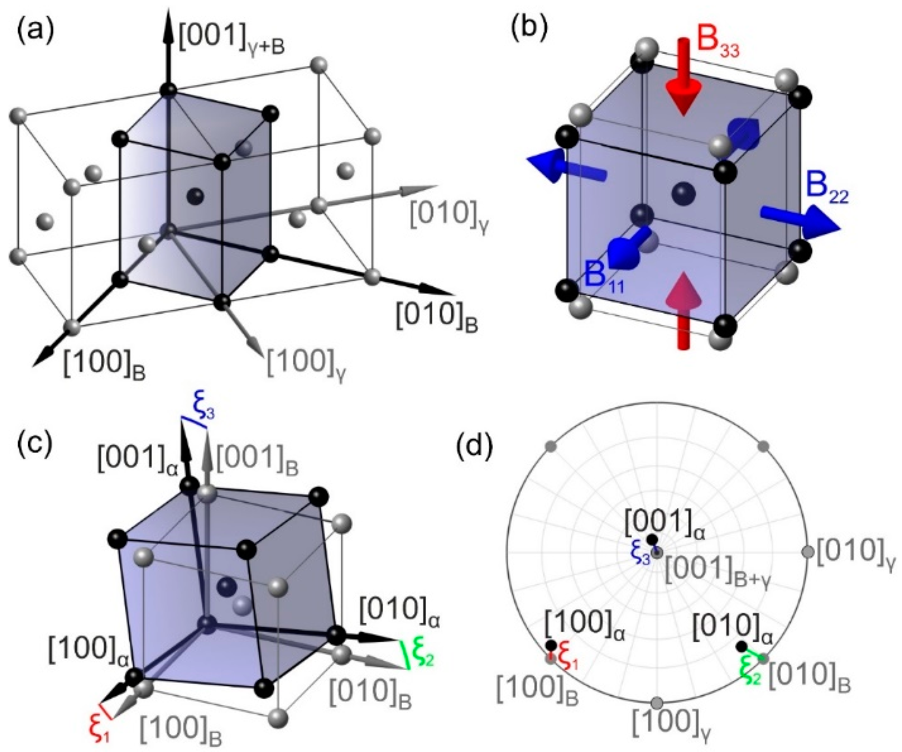
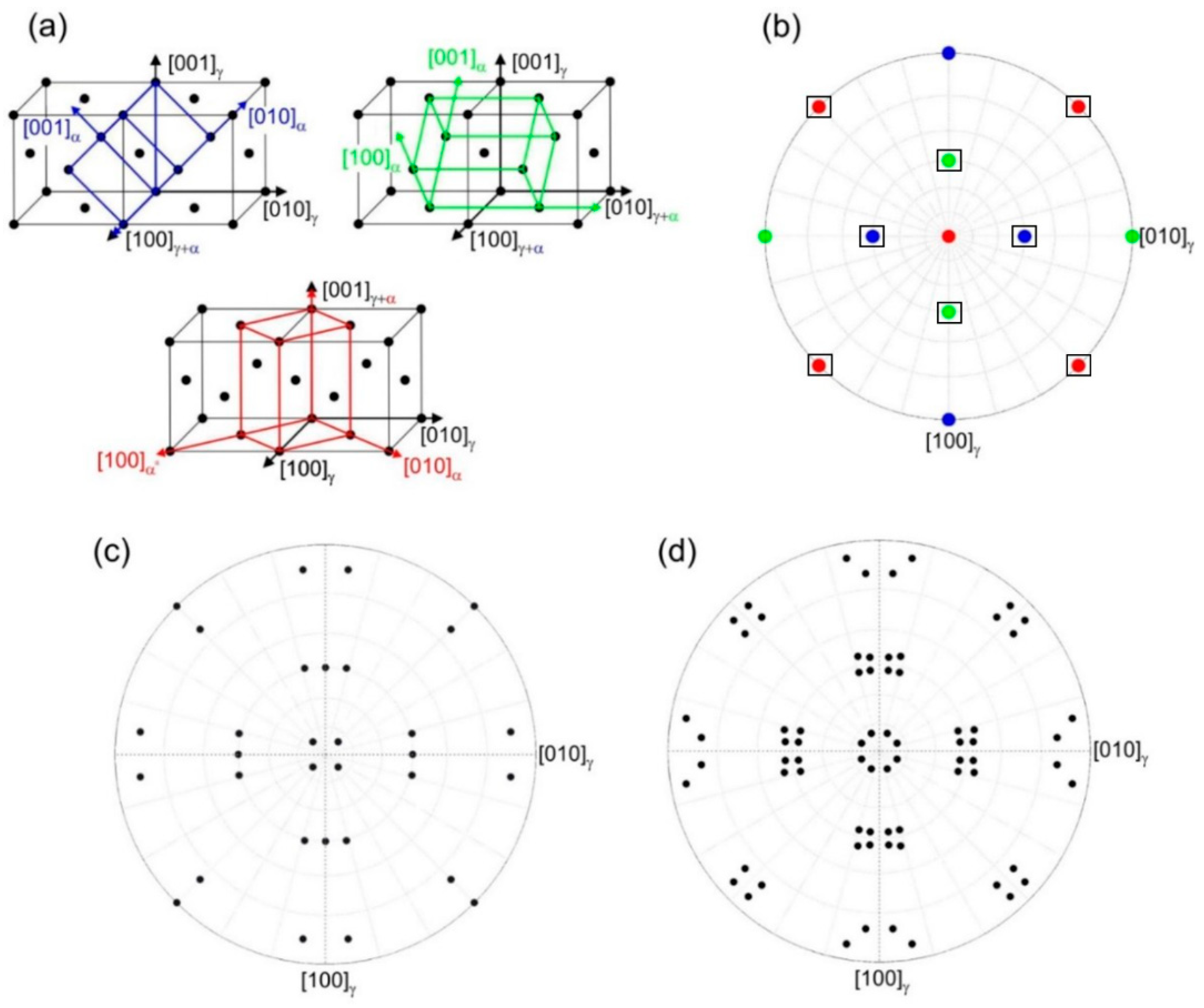
2.2. Martensite Crystallography and Evaluation of EBSD Data

Crystallographic relations between martensite and austenite: Figure 3 shows four schematic drawings, which help to appreciate the crystallographic relations between austenite and martensite. Figure 3a–d can be thought of as a sequence, which schematically illustrates the individual crystallographic steps involved in a martensitic transformation from austenite γ to martensite α’. The crystallographic differences between the lattices of the cubic-body centered ferrite α and tetragonal distorted martensite α’ are so small that they can be neglected in our analysis—where we only consider bcc α. In all schematic drawings presented in Figure 3, the positions/orientations of the initial configuration are illustrated using grey spheres, while the subsequent configuration is shown using black spheres. The black symbols representing the final configuration in one figure are used as the starting configuration (in grey) in the next figure.
Figure 3a shows the original Bain correspondence [3], which represents a 45° rotation of the original coordinate system (grey) around the [001] γ-axis—which remains at the [001] axis in α. It is well known that three Bain strains, B11, B22 (B11 = B22, both tensile), and B33 (compressive), are required to transform the tetragonal distorted grey configuration in Figure 3a into a regular bcc atom arrangement, represented in Figure 3b. Figure 3c shows that the actual orientation relationship (black coordinate system) deviates from the ideal Bain situation (grey coordinate system) by the three angles ξ1, ξ2, and ξ3, where the indices 1, 2, and 3 correspond to the x, y, and z-axes of the Bain cell. These deviations were already experimentally detected by Kurdjumov/Sachs [4] and Nishiyama/Wassermann [5,6] a century ago. In the framework of the phenomenological theory of the martensitic transformation (PTMT), they result from the need for the presence of an invariant martensite/austenite interface [7]. Mathematically, they manifest themselves as a rigid body rotation, which, in combination with the cubic symmetry elements, leads to the formation of 12 (ξ1 = 0) and 24 (ξ1 > 0) MVs, respectively. Figure 3d shows the directions and angles from Figure 3c in a pole figure.
The transformation steps illustrated in Figure 3a–c can be mathematically expressed using transformation matrices, which capture the essence of the PTMT [7]. In passing, we note that the derivation of the PTMT was based on the observation that the measured ORs between austenite and martensite do not precisely match the plane parallelism of the KS nor of the NW ORs. It is common to use the sphere/ellipsoid transformation to analyze the micromechanics of the transformation [9]. If a sphere of unit radius represents the fcc structure, then, after the Bain distortion, it will represent an ellipsoid with two axes expanded and a third axis contracted. As a result, in this scenario there is no habit plane that remains fully undistorted after transformation. The key to the crystallographic theory of the martensitic transformation is to postulate that the additional shear strains compensate for this incompatibility, resulting in the slight rotations shown in Figure 3c.
The sequence of images presented in Figure 3 is based on an initial γ and a final α configuration. The habit plane of martensite can be defined as a plane in the austenite that undergoes no net (macroscopic) distortion and rotation. By net distortion and rotation, it is meant that the distortion, when averaged over many martensite variants, is zero. Figure 3 provides a frame which allows crystallographic relations to be appreciated. It must be kept in mind, however, that it does not directly represent the sequence of events that govern the transformation. In our EBSD analysis we follow the mathematical procedure, which was qualitatively outlined by Yardley and Payton [45]. Matrix algebra is used to separate the different transformation processes, such as axis transformations (Figure 3a), symmetry elements (not shown in Figure 3), and strains (Figure 3b), from physically relevant rigid body rotations (Figure 3c,d). We now have to address the fact that EBSD indexation typically provides one arbitrary valid representation for one measurement. This can make it difficult to relate martensite variant orientations to the parent austenite lattice. Our mathematical treatment overcomes this problem. It first requires us to relate the coordinate systems of all 24 martensite variants to all valid austenite coordinate systems. It must be kept in mind that for symmetry reasons, cubic systems (fcc and bcc) can be described by 24 valid coordinate systems. Equation (3) allows for all MV orientations to be rationalized with respect to the parent austenite lattice:
D M Θ M    ( v , s ) = Ω M      ( s ) Ξ B Γ Ω A ( v ) D A Θ A
The expression DMθM(v,s) describes the base vectors of all potential MVs, v (v: first variant run parameter; iteration over integer values from 1 to 24) together with all symmetric equivalents s (s: second coordinate system run parameter; iteration over integer values of from 1 to 24). DM is a diagonal matrix with the lattice parameters of the α-phase in the direction of the base vectors of the ferritic unit cell (all equal in cubic systems). ΘM represents the rotation matrix describing the orientations of all MVs. ΘA, on the right side of Equation (3), describes the initial austenite orientation. DA represents the lattice parameters of the γ-phase. ΩA(v) and ΩA(s) each comprise 24 equivalent representations (in both cubic crystal lattices each orientation can be described using 24 distinct orthonormal coordinate systems). The Bain correspondence illustrated in Figure 3a is captured in the matrix Γ. The matrix B contains elements which stand for the Bain strains, shown in Figure 3b. The matrix Ξ represents the rigid body rotation shown in Figure 3c,d. This allows for all MV orientations that can form within one austenite grain to be found.
Before we proceed, we take a closer look at the established orientation relationships. First, as can be seen in Figure 4a, there are three Bain correspondences, which highlighted in blue, green, and red. These correspond to three possible MV orientations, which are shown in the same color coding in the pole figure of Figure 4b. The special case outlined in Figure 4a,b corresponds to a situation where the three characteristic angles ξ1, ξ2, and ξ3 are all equal to zero. In the case of the NW orientation relationship, the angle ξ1 is zero while ξ2 = ξ3 > 0. The resulting <100> axes of the twelve NW MVs are shown in Figure 4c. We note that only the <100>, highlighted in Figure 4b, reappear in Figure 4c. In the case of the NW relationship, each Bain correspondence allows four possible permutations, resulting in twelve distinct MVs. In contrast, for the KS orientation relationship, where all three angles differ from zero and from each other, one obtains the pole figure shown in Figure 4d. Here we find 24 variants, which can be considered as the general 24 variant case. The ξ-parameters, which were introduced in Figure 3c,d, not only allow for the description of the NW and KS orientation relationships (Figure 4c,d) as special cases, but they also define a space, which provides a framework allowing for arbitrary ORs and the dispersion of ORs to be quantified in a given microstructure.
Analysis of EBSD data: We now apply the crystallographic relations described above to analyze the EBSD data from martensitic microstructures. Martensitic microstructures consist of multiple variants with different orientations, which do not directly reveal the orientation of the parent austenite grains. However, for each MV, we can calculate the orientations of all potential austenite parent lattices. Equation (4) (an inversion of Equation (3)) provides this information:
Θ A ( v , s ) k = D A 1 Ω A ( v ) 1 Γ 1 B 1 Ξ 1 Ω M ( s ) 1 D M Θ k M
where all parameters and operators are described above, except the subscript k, which stands for the individual EBSD data points and represents a run parameter that extends from 1 to approximately 500,000 (total number of orientation measurements). Here we assume that all data points describe the orientations of MV that have formed within one common austenite grain. The orientation of this austenite grain can be obtained using a probabilistic approach. This approach involves the evaluation of the superposition of all arithmetically possible austenite orientations using an orientation density function (ODF) and is implemented in the MTEX toolbox for MATLAB [50,51,52]. The ODF calculations are based on spherical harmonics, and we use color-coded density pole figures (PDFs—pole density figures) to visualize the ODF calculations. The maximum value of this ODF represents the most likely prior austenite orientation and is given by Equation (5):
Θ A = k Θ A ( v , s ) k
where the large, sharp outer brackets indicate that the ODF needs to be evaluated to retrieve the dominant orientation. This is graphically illustrated in Figure 5a–c.
Figure 5a shows the IPF map of the martensitic microstructure of Fe28Ni (directions: see color coded standard triangle inset), which was retrieved from 500,000 measurements. In the pole figure shown in Figure 5b, a qualitative blue (low density) to green and red (high density) color coding is used to indicate the density of the calculated austenite crystal orientations. Figure 5b also shows the density of the unit vectors of all original MVs (distinct data points appearing as grey data clouds). It can be clearly seen that there are distinct maxima, which are associated with one austenite crystal lattice orientation. These maxima are interpreted as actual orientations in Figure 5c (red points) together with the underlying experimental martensite data (grey data clouds).
To determine parameters that identify the nature of ORs, we rotate the EBSD data set into a <100> austenite standard projection, shown in Figure 6a. This is achieved by calculating the inverse of ΘA (defined in Equation (3)). This inversion, ΘA−1, accounts for the required rotation. The red poles in Figure 6a represent the <100>γ austenite axes; the experimental <100>α martensite axes are shown as grey point clouds. By applying the symmetry elements ΩM(s) and ΩA(v) (see Equation (3)), one can project all k (run parameter in Equation (2)) EBSD results into one fundamental zone. This allows one representative MV to be obtained, which needs to be represented as a standard projection considering the Bain correspondence. This requires the rotation described by Γ−1 (see Equation (4)).
Thus, one obtains a new ODF, which directly reflects the orientation relationship between the Bain correspondence and the representative MV, shown in Figure 6b. Figure 6b represents a color-coded visualization (low/high densities: blue/yellow, as indicated) of the ODF, where the grey dots correspond to the Bain axes shown in Figure 3a and Figure 4a. The three ODF maxima shown in Figure 6b reflect the crystal axes of the representative MVs relative to the Bain correspondence. The differences between the experimental orientations and the precise Bain orientations characterize the orientation relationship and correspond to the parameter Ξ from Equations (3) and (4), which quantifies the rigid body rotation described above and illustrated in Figure 3c,d. The cosine functions of the diagonal elements of Ξ yield the three characteristic angles ξ1, ξ2, and ξ3 from Figure 3c,d. One can now reinsert this experimental Ξ into Equation (1) to obtain the average orientation relationship between austenite and martensite, shown in Figure 6c (red poles: <100>γ, black crosses: orientation relationship considering 24 MVs). Note that when the prior austenite orientation was initially calculated, we used a reasonably chosen Ξ—matrix, while the results shown in Figure 6c represent the best fit of the experimental data. In Figure 6d, we introduce color-coding, which allows us to differentiate between different MV orientations.

3. Results

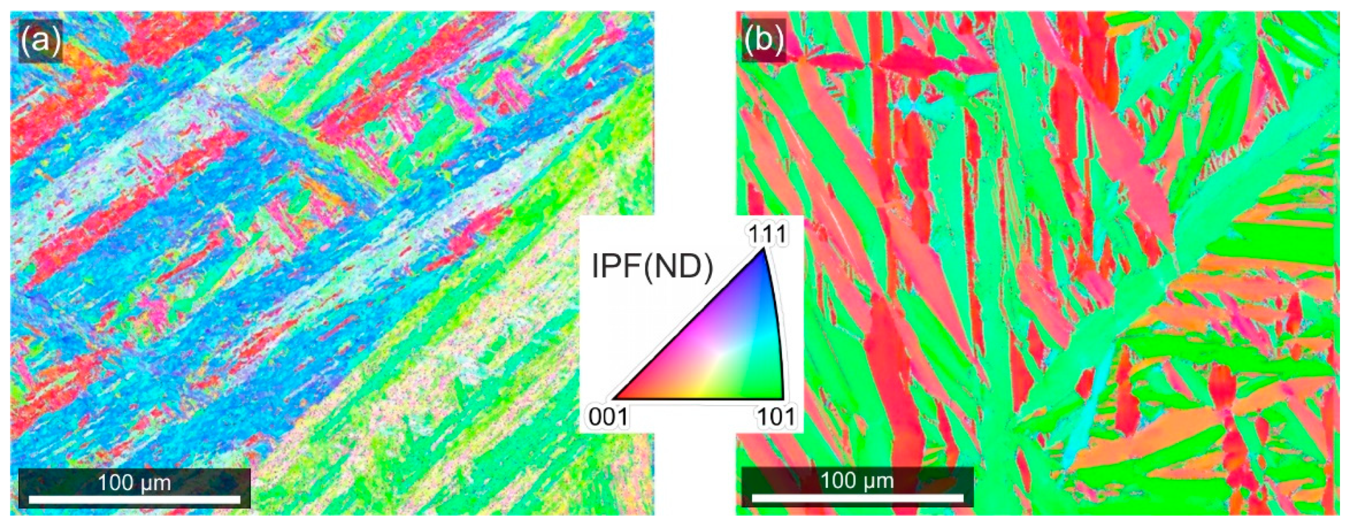
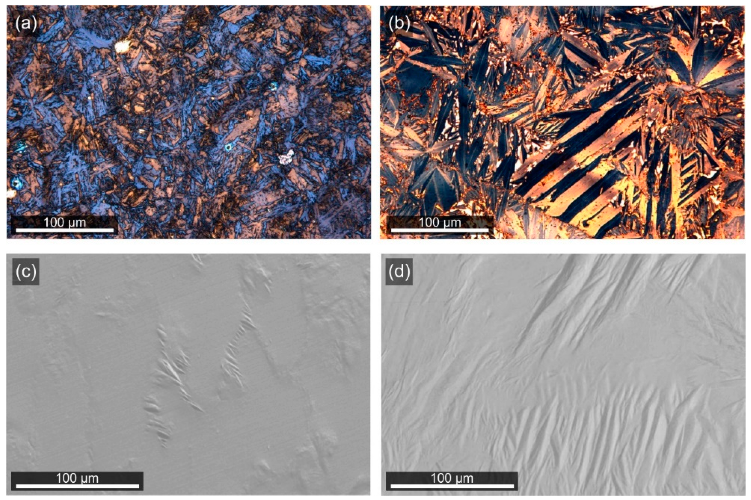
3.1. Martensite Microstructures

We now apply the OI-EBSD procedure outlined above to show the microstructures of the two types of martensite that we consider in the present work. Figure 7a,c show lath martensite data and the results for plate martensite are presented in Figure 7b,d. Figure 7a,b show color-coded microstructures as specified in Figure 6d. Figure 7c,d show corresponding misorientation angles between the average and measured MV orientations, which are color coded as indicated on the bottom of Figure 7. Figure 7a,c show results obtained for a system that shows the lath type of transformation behavior (Fe-27.5Ni). The microstructure shows fine needle-like martensite crystals, which are arranged in blocks with highly serrated block boundaries—one is highlighted with a white arrow. Figure 7a shows that LM exhibits a finely dispersed distribution of short-range deviations from average orientations. The results for the pure PM in Fe-29.5Ni are presented in Figure 7b,d. PM shows some larger crystals with straight, non-parallel boundaries—one is highlighted with a white arrow—together with smaller crystals occupying the spaces between them. Figure 7d shows a spatial mapping of local deviations from average orientations. The difference between the deviation plots in Figure 7c (LM) and Figure 7d (PM) is obvious. The deviation plot of PM allows us to appreciate the presence of midribs, two of which are marked with white arrows. The plot also shows that angular deviations increase as one moves from the center of a plate towards its outer boundary.

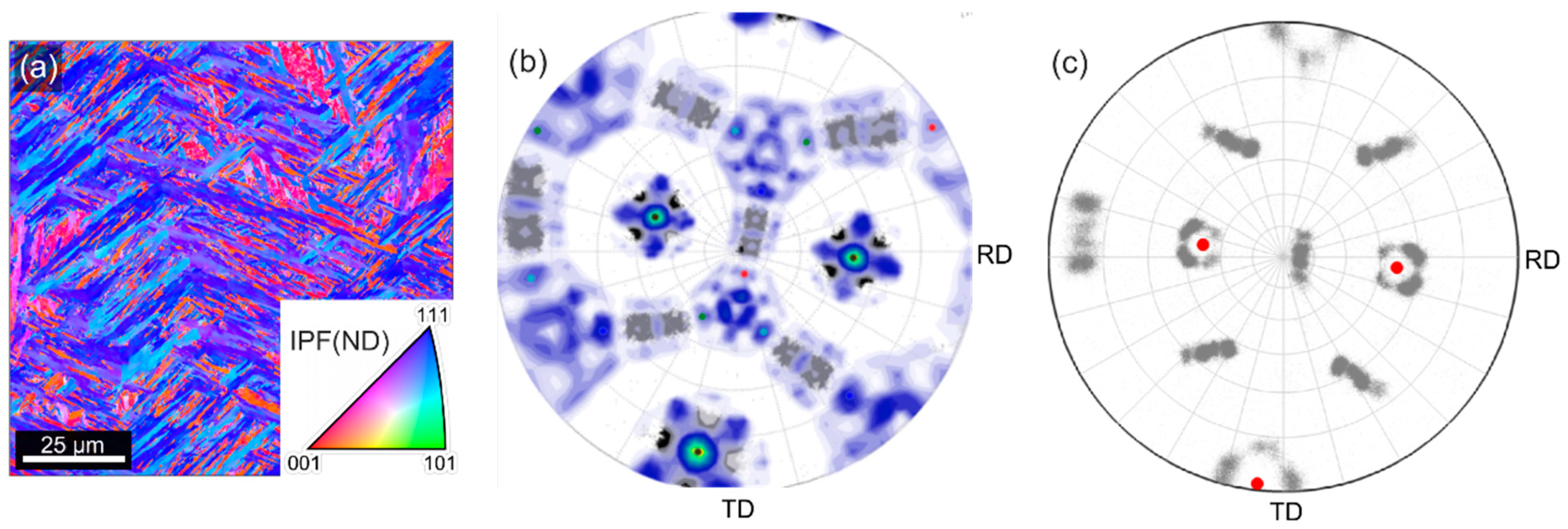
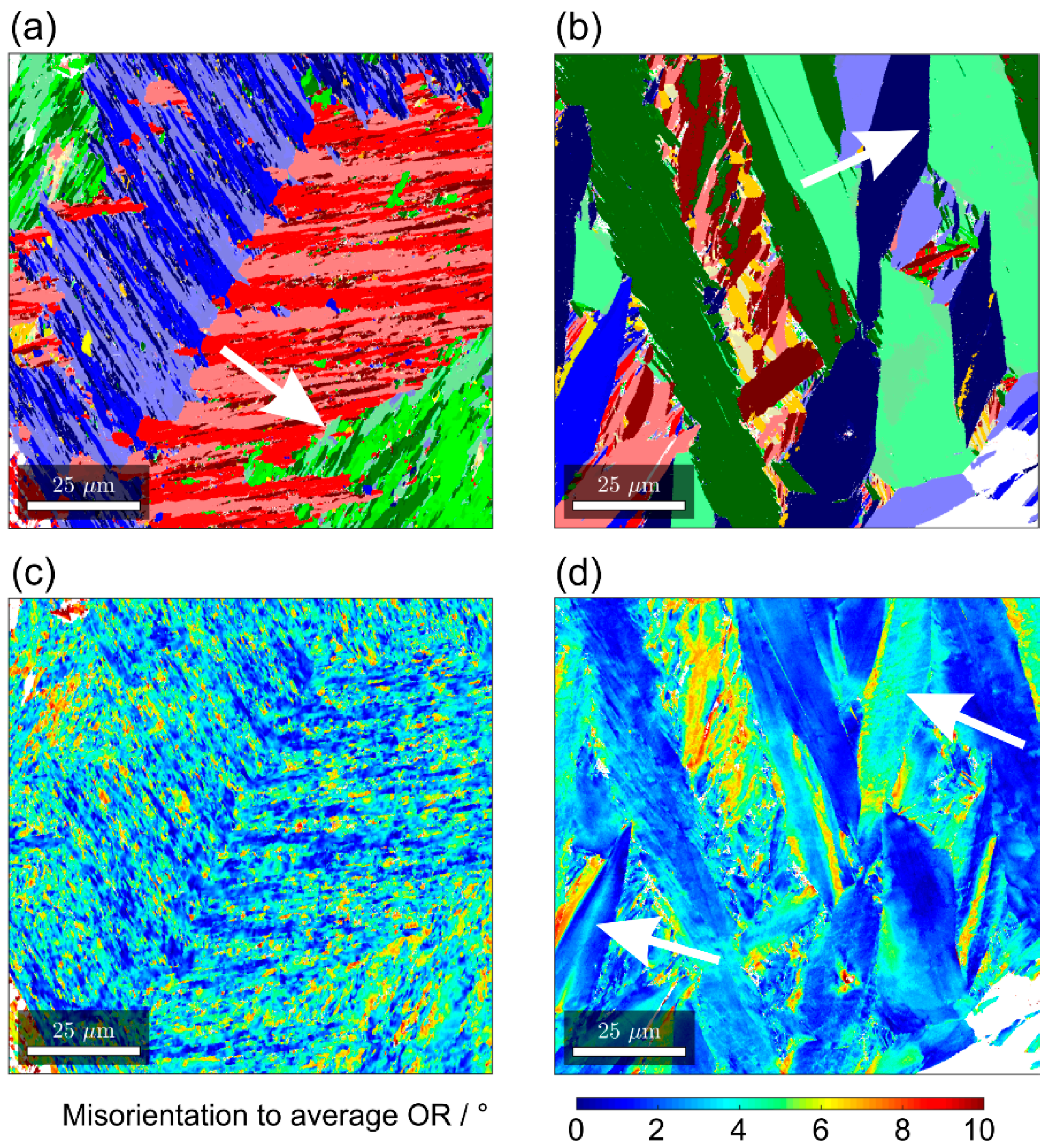
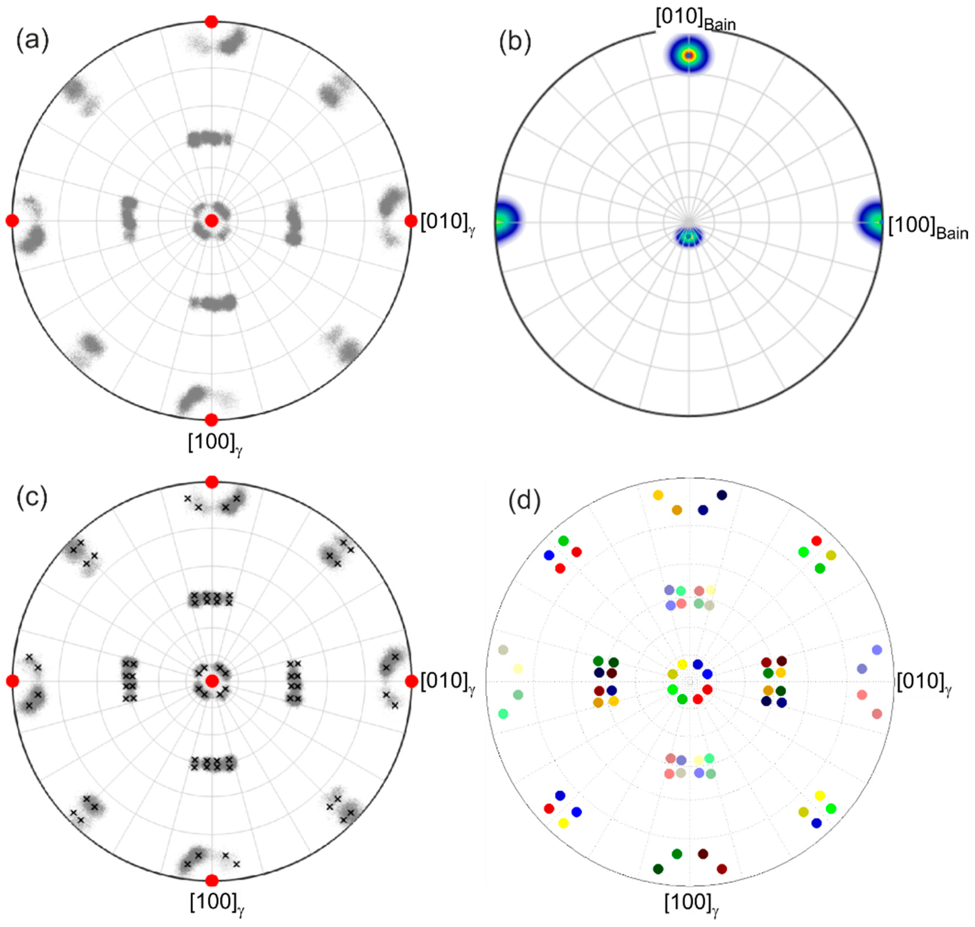
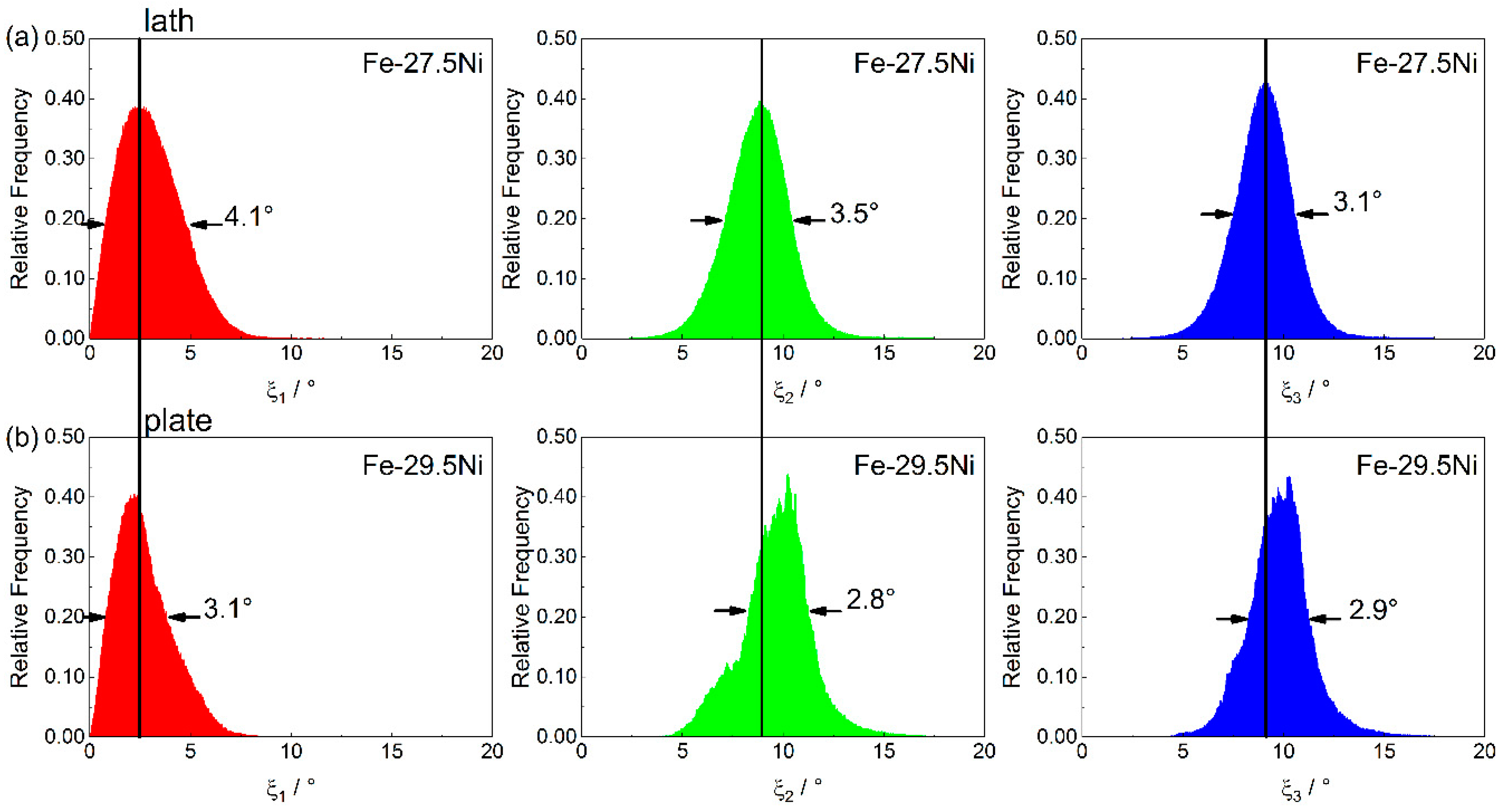
3.2. Statisticaal Analysis of the OR

In Figure 8, we present the relative frequency distributions of the three characteristic angles ξ1, ξ2, and ξ3. The distributions of the ξ angles are smooth and have a near-Gaussian appearance. However, one can identify the differences in the ξ angle distributions in the two martensite microstructures. For both types of distributions, we can quantify the angular position of the maximum and the full width at half maximum (FWHM). As far as ξ1 is concerned, one finds no significant differences in terms of angular distances from zero. However, the LM peak is smooth and broad, as shown in Figure 8a. In contrast, the PM shows a narrower and sharper peak, as shown in Figure 8b.
For the angles ξ2 and ξ3 one finds that FWHMLM > FWHMPM. When taking the angular maxima positions of LM as a reference, one can see that maxima for the PM are slightly shifted to the right. In Figure 9, we show pole figures that are presented in a [100] austenite reference system. Figure 9a,b show the measured [100]α’ directions of all the detected MVs (grey data points forming data clouds). The figures include the [100]α’ directions corresponding to the NW (red points) and KS (green points) ORs, which are described in Figure 4c,d. In addition, the corresponding directions representing the Greninger–Troiano OR (GT, [53], not considered so far) are shown.

4. Discussion

The fact that analytical EBSD can provide new insight into the microstructural details of martensitic microstructures is not new. Thus, Shibata et al. [54,55] showed that, in a Fe-33 at.% Ni alloy along a midrib of a martensite plate, the local orientations gradually change by up to 3° when moving from the center to the outside of a lenticular martensite plate, which is similar to what we see in Figure 7d. Sato and Zaefferer [56] report the presence of a butterfly type of martensite in a Fe-30 at.% Ni alloy and relate its formation to the dislocation processes in the austenite phase. Yardley and Payton [45] suggested that local variations of MV orientations from average orientation relationships are no experimental artefact, but instead help to reveal microstructural details, as we also show in the present work in Figure 7c,d. Their method was applied to study creep crack growth in tempered martensite ferritic steels [57] and is still being explored [58,59]. Thus, it was recently extended to explore the accuracy and efficacy of a Bayesian approach for describing the austenite–to–martensite orientation relationship [59]. Using the prior austenite orientation as a reference frame eliminates ambiguous contrasts in the microstructure that appear in standard IPF-EBSD-mappings, such as those shown in Figure 1, where the prior austenite orientation affects the appearance of individual MVs.
Using the distributions of the three characteristic angles ξ1, ξ2, and ξ3, one can gain further insight into the nature of the martensitic transformation. Thus, as was shown in Figure 8, one can identify the two different types of martensite by the widths of the distributions of the characteristic angles. Our approach differs from other approaches in that it does not relate the measured variant orientations to the idealized orientation relationships, such as KS and NW [60]. There is no general agreement in the literature on whether different ORs can rationalize martensitic microstructures [61,62] or whether there is only one unique OR that governs the relative orientations of the parent and product phase [63,64]. Our statistical analysis can help in this respect. In Figure 9, we show our experimental data for the two martensite structures LM and PM together with the ORs of KS [4], NW [5], and Greninger and Troiano [53]. For both martensite microstructures detected in the present work, the three ORs fall within the experimental data clouds that result from a statistical distribution of local orientations related to microstructural evolution during the transformation and deformation processes, as shown in Figure 9. The final orientation of each martensite crystal is not only governed by the tendency to establish a most favorable OR; it also relies on local distortions between the parent and product phase, which govern its nucleation and growth. Dislocation stress fields also play a role. Further work is required to explore these local effects. Our results show that these superimposed micromechanical effects make it difficult to distinguish between the three idealized ORs (KS, NW, and GT), which are all reasonably close to the experimental data. Our results provide clear experimental evidence that shows that real martensite microstructures cannot be rationalized by precise crystallographic ORs.

5. Conclusions

In the present work, we used an advanced EBSD procedure to study the two types of martensitic microstructures that are observed in the Fe-Ni system, lath martensite (below 28.5 at.% Ni) and plate martensite (above 28.5 at.% Ni). We modify, document, and apply an analytical EBSD procedure that was originally proposed by Yardley and Payton 2014 [45]. It analyzes the distributions of the three angles ξ1, ξ2, and ξ3, which describe the small angular deviations between the crystal planes in the unit cells of martensite and austenite—which are related through specific orientation relationships. The analysis of the angular distributions can be exploited to obtain high-resolution, color-coded micrographs of martensitic microstructures, which, for example, visualize the midribs in large plates of a plate martensite microstructure. The differences between the two major types of martensite (lath and plate) also manifest themselves in the differences in the full widths at half maxima (wide for lath martensite, narrow for plate martensite) in the ξ distributions.
Our analysis also allows for a contribution to the longstanding debate on which orientation relationship between austenite and martensite is relevant and whether or not one can detect more than one orientation relationship in one martensitic microstructure. The data obtained in the present work show that when the experimental martensitic crystallographic data are presented in [100] austenite reference pole figures, the [100]α’ directions of many martensite variants form local data clouds. For both martensite microstructures detected in the present work, the predictions of the three prominent orientation relationships (Kurdjumov–Sachs, Nishiyama–Wassermann and Greninger–Troiano) fall within these experimental data clouds. The data clouds result from a statistical distribution of the local orientations. The orientation of each martensite crystal is not only affected by the tendency to establish one specific OR. Other factors are important and are associated with the distortions between adjacent variants and with the strain fields of lattice defects. Our results clearly show that these superimposed micromechanical effects that affect martensite variant crystal orientations overrule the possibility to precisely distinguish between specific orientation relationships. Figure 7 and Figure 9 show that the intrinsic distribution of MV orientations, which is caused by local deformations, exceed the angular difference between specific named ORs. Therefore, different ORs can be determined within one martensite structure, depending on where the OR was measured. There are different possibilities of defining a representative OR for a given material (e.g., average OR, OR at MV interfaces, OR at austenite-martensite interface, OR at midrib with respect to prior austenite orientation, etc.). Further work is required to clarify the exact definition of a meaningful representation of an OR.

Author Contributions

Conceptualization, V.A.Y. and E.J.P.; methodology, V.A.Y., E.J.P. and P.T.; software, V.A.Y., E.J.P. and P.T.; validation, P.T.; formal analysis, P.T. and M.S. investigation, P.T. and M.S.; resources, V.A.Y., E.J.P.; data curation, P.T.; writing—original draft preparation, P.T. and G.E.; writing—review and editing, V.A.Y. and E.J.P.; visualization, P.T. and V.A.Y.; supervision, G.E.; project administration, V.A.Y. and P.T.; funding acquisition, V.A.Y. and E.J.P. All authors have read and agreed to the published version of the manuscript.

Funding

The authors acknowledge funding by the German Research Association (DFG) through projects YA 326/2-1 (PT, MS, VAY), PA 2285/1-1 (EP), and SFB/TR 103-A2 (GE).

Data Availability Statement

Not applicable.

Conflicts of Interest

The authors declare no conflict of interest.

References

  1. Osmond, F. Méthode générale pour l’analyse micrographique des aciers au carbone. Bulletin de la Société d’Encouragement pour l’indutrie Nationale 1895, 10, 476–518. [Google Scholar]
  2. Martens, A. Über das Kleingefüge des schmiedbaren Eisens, besonders des Stahles. Stahl Eisen 1887, 7, 235–242. [Google Scholar]
  3. Bain, E.C.; Dunkirk, N.Y. The nature of martensite. Trans. AIME 1924, 70, 25–46. [Google Scholar]
  4. Kurdjumow, G.; Sachs, G. Über den Mechanismus der Stahlhärtung, Z. Physik 1930, 64, 325–343. [Google Scholar] [CrossRef]
  5. Nishiyama, Z. X-ray investigation of the mechanism of the transformation from face-centred cubic lattice to body-centred cubic, Science Reports of the Tohoku Imperial University, Series 1: Mathematics. Phys. Chem. 1934, 23, 637–664. [Google Scholar]
  6. Wassermann, G. Über den Mechanismus der α/γ-Umwandlung des Eisens; Mitteilungen aus dem Kaiser-Wilhelm-Institut für Eisenforschung zu; Verlag Stahleisen: Düsseldorf, Germany, 1935. [Google Scholar]
  7. Wechsler, M.S.; Liebermann, D.S.; Read, T.A. On the theory of the formation of martensite. Trans. AIME 1953, 197, 1503–1515. [Google Scholar]
  8. Knapp, H.; Dehlinger, U. Mechanik und Kinetik der diffusionslosen Martensitbildung. Acta Metall. 1956, 4, 289–297. [Google Scholar] [CrossRef]
  9. Wayman, C.M. Introduction to the crystallography of martensitic transformations. Macmillan Siries Mater. Sci. 1964. [Google Scholar]
  10. Nishiyama, Z. Martensitic Transformation; Academic Press: London, UK, 1978. [Google Scholar]
  11. Olson, G.B.; Owen, W.S. Martensite—A Tribute to Morris Cohen. ASM Int. 1992. [Google Scholar]
  12. Wayman, C.M.; Bhadeshia, H.K.D.H. Nondiffusive phase transformations. In Physical Metallurgy, 4th ed.; Cahn, R.W., Haasen, P., Eds.; North-Holland: Amsterdam, The Netherlands, 1996; Volume 2, pp. 1507–1554. [Google Scholar]
  13. Christian, J.E. The Theory of Transformations in Metals and Alloys; Parts 1 and 2; Pergamon: Amsterdam, The Netherlands, 2002. [Google Scholar]
  14. Kraus, G.; Marder, A.R. The morphology of martensite in iron alloys. Met. Trans. 1971, 2, 2343–2357. [Google Scholar] [CrossRef]
  15. Pereloma, E.; Edmonds, D.V. Phase Transformations in Steels: Diffusionless Transformations; Woodhead Publishing: Cambridge, UK, 2012. [Google Scholar]
  16. Kelly, P.M.; Nutting, J. The morphology of martensite. J. Iron Steel Inst. 1961, 197, 199–211. [Google Scholar]
  17. Speich, G.R.; Swann, P.R. Yield strength and transformation substructure of quenched iron nickel alloys. J. Iron Steel Inst. 1965, 203, 480–485. [Google Scholar]
  18. Owen, W.S.; Wilson, E.A.; Bell, T. High Strength Materials; John Wiley and Sons: New York, NY, USA, 1965; pp. 167–208. [Google Scholar]
  19. Morito, S.; Huang, X.; Furuhara, T.; Maki, T.; Hansen, N. The morphology and crystallography of lath martensite in alloyed steels. Acta Mater. 2006, 54, 5323–5331. [Google Scholar] [CrossRef]
  20. Patterson, R.L.; Wayman, C.M. Crystallography and growth of partially-twinned martensite plates in Fe-Ni alloys. Acta Metall. 1966, 14, 347–369. [Google Scholar] [CrossRef]
  21. Krauss, G. Martensite in steel: Strength and structure. Mat. Sci. Eng. A 1990, 273, 40–57. [Google Scholar] [CrossRef]
  22. Kitahara, H.; Ueji, R.; Ueda, M.; Tsuji, N. Minamino, Crystallographic analysis of plate martensite in Fe-28.5 at.% Ni by FE-SEM/EBSD. Mater. Charact. 2005, 54, 378–386. [Google Scholar] [CrossRef]
  23. Kitahara, H.; Ueda, M.; Tsuji, N. Minamino, Variant selection of plate martensite in Fe-28.5 at.% Ni alloy. Mater. Sci. Forum 2006, 512, 117–121. [Google Scholar] [CrossRef]
  24. Hansen, M.; Anderko, K. Constitution of Binary Alloys; McGraw-Hill Book Company: New York, NY, USA, 1958. [Google Scholar]
  25. Swartzendruber, L.J.; Itkin, V.P.; Alcock, C.B. The iron-nickel system. J. Phase Equilibria 1991, 12, 288–312. [Google Scholar] [CrossRef]
  26. Schwartz, A.J.; Kumar, M.; Adams, B.L. Electron. Backscatter Diffraction in Materials Science; Kluwer Academic Publishers: New York, NY, USA, 2000. [Google Scholar]
  27. Randle, V.; Engler, O. Introduction to Texture Analysis: Macrotexture, Microtexture, and Orientation Mapping, 2nd ed.; CRC Press: London, UK, 2009. [Google Scholar]
  28. De Graef, M.; McHenry, M. Structure of Materials–An Introduction to Crystallography, Diffraction and Symmetry, 2nd ed.; Cambridge University Press: Cambridge, UK, 2012. [Google Scholar]
  29. Nishikawa, S.; Kikuchi, S. The diffraction of cathode rays by calcite. Proc. Imp. Acad. Jpn. 1928, 4, 475–477. [Google Scholar] [CrossRef] [Green Version]
  30. Von Heimendahl, M.; Bell, W.; Thomas, G. Applications of Kikuchi Line Analyses in Electron Microscopy. J. Appl. Phys. 1964, 35, 3614–3616. [Google Scholar] [CrossRef]
  31. Boersch, H.; Zeitschrift, P. About bands in electron diffraction. Phys. Z. 1937, 38, 1000–1004. [Google Scholar]
  32. Reimer, L. Scanning Electron Microscopy—Physics of Image Formation; Springer: Berlin, Germany, 1985. [Google Scholar]
  33. Dingley, D.J.; Randle, V. Microtexture determination by electron back-scatter detection. J. Mater. Sci. 1992, 27, 4545–4566. [Google Scholar] [CrossRef]
  34. Adams, B.L.; Wright, S.I.; Kunze, K. Orientation imaging–the emergence of a new microscopy. Metall. Trans. A 1993, 24, 819–831. [Google Scholar] [CrossRef]
  35. Gourgues, A.-F.; Flower, H.M.; Lindley, T.C. Electron back scattering diffraction study of acicular ferrite, bainite and martensite steel microstructures. Mater. Sci. Tech. 2000, 16, 26–40. [Google Scholar] [CrossRef]
  36. Morito, S.; Tanaka, H.; Konishi, R.; Furuhara, T.; Maki, T. The morphology and crystallography of lath martensite in Fe-C alloys. Acta Mater. 2003, 51, 1789–1799. [Google Scholar] [CrossRef]
  37. Kitahara, H.; Ueji, R.; Tsuji, N.; Minamino, Y. Crystallographic features of lath martensite in low carbon steel. Acta Mater. 2006, 54, 1279–1288. [Google Scholar] [CrossRef]
  38. Cayron, C.; Artaud, B.; Briottet, L. Reconstruction of parent grains from EBSD data. Mater. Charact. 2006, 57, 386–401. [Google Scholar] [CrossRef]
  39. Miyamoto, G.; Iwata, N.; Takayama, N.; Furuhara, T. Mapping the parent austenite orientation reconstructed from the orientation of martensite by EBSD. Acta Mater. 2010, 58, 6393–6403. [Google Scholar] [CrossRef]
  40. Miyamoto, G.; Takayama, N.; Furuhara, T. Accurate measurement of the orientation relationship of lath martensite and bainite by electron backscatter diffraction analysis. Scr. Mater. 2009, 60, 1113–1116. [Google Scholar] [CrossRef]
  41. Pham, A.H.; Ohba, T.; Morito, S.; Hayashi, T. Effect of chemical composition on average γ/α’ orientation relationship in carbon and low alloy steels. Mater. Today Proc. 2015, 2S, 663–666. [Google Scholar] [CrossRef]
  42. Zilnyk, K.D.; Junior, D.R.A.; Sandim, H.R.Z.; Rios, P.R.; Raabe, D. Misorientation distribution between martensite and austenite in Fe-31 wt% Ni-0.01 wt% C. Acta Mater. 2018, 143, 227–236. [Google Scholar] [CrossRef]
  43. Germain, L.; Gey, N.; Mercier, R.; Blaineau, P.; Humbert, M. An advanced approach to reconstructing parent orientation maps in the case of approximate orientation relations: Application to steels. Acta Mater. 2012, 60, 4551–4562. [Google Scholar] [CrossRef]
  44. Niessen, F.; Nyyssönen, T.; Gazder, A.A. Hielscher, Parent grain reconstruction from partially or fully transformed microstructures in MTEX. arXiv 2021, arXiv:2104.14603. [Google Scholar]
  45. Yardley, V.A.; Payton, E.J. Austenite-martensite/bainite orientation relationship: Characterization parameters and their application. Mat. Sci. Technol. 2014, 30, 1125–1130. [Google Scholar] [CrossRef] [Green Version]
  46. Frenzel, J.; George, E.P.; Dlouhy, A.; Somsen, C.; Wagner, M.F.X.; Eggeler, G. Influence of Ni on martensitic phase transformations in NiTi shape memory alloys. Acta Mater. 2010, 58, 3444–3458. [Google Scholar] [CrossRef]
  47. Rahim, M.; Frenzel, J.; Frotscher, M.; Pfetzing-Micklich, J.; Steegmüller, R.; Wohlschlögel, M.; Mughrabi, H.; Eggeler, G. Impurity levels and fatigue lives of pseudoelastic NiTi shape memory alloys. Acta Mater. 2013, 61, 3667–3686. [Google Scholar] [CrossRef]
  48. Thome, P. Advancing orientation imaging scanning electron microscopy (in German). Ph.D. Thesis, Ruhr-Universität, Bochum, Germany, 2019. [Google Scholar]
  49. Benscoter, A.O. Carbon and alloy steels. In Metallography and Microstructures; Vander Voort, G.F., Ed.; ASM International: Novelty, OH, USA, 2004; Volume 9, pp. 165–196. [Google Scholar]
  50. Benker, H. Mathematik mit MATLAB; Springer: Berlin/Heidelberg, Germany, 2000. [Google Scholar]
  51. Hielscher, R.; Schaeben, H. A novel pole figure inversion method: Specification of the MTEX algorithm. J. Appl. Cryst. 2008, 41, 1024–1037. [Google Scholar] [CrossRef]
  52. Bachmann, F.; Hielscher, R.; Schaeben, H. Texture analysis with MTEX—Free and open source software toolbox. Solid State Phenom. 2010, 160, 63–68. [Google Scholar] [CrossRef] [Green Version]
  53. Greninger, B.; Troiano, A.R. The mechanism of martensitic transformation. J. Metall. Trans. 1949, 185, 590–598. [Google Scholar]
  54. Shibata, A.; Morito, S.; Furuhara, T.; Maki, T. Substructures of lenticular martensites with different martensite start temperatures in ferrous alloys. Acta Mater. 2009, 57, 483–492. [Google Scholar] [CrossRef]
  55. Shibata, A.; Morito, S.; Furuhara, T.; Maki, T. Local orientation change inside lenticular martensite plate in Fe-33Ni alloy. Scr. Mater. 2005, 53, 597–602. [Google Scholar] [CrossRef]
  56. Sato, H.; Zaefferer, S. A study on the formation mechanism of butterfly-type martensite in Fe-30%Ni alloy using EBSD-based orientation microscopy. Acta Mater. 2009, 57, 1931–1937. [Google Scholar] [CrossRef]
  57. Yardley, V.A.; Fahimi, S.; Payton, E.J. Classification of creep crack and cavitation sites in tempered martensite ferritic steel microstructures using MTEX toolbox for EBSD. Mater. Sci. Technol. 2015, 31, 547–553. [Google Scholar] [CrossRef]
  58. Brust, A.F.; Niezgoda, S.R.; Yardley, V.A.; Payton, E.J. Analysis of misorientationrelationships between austenite parents and twins. Metall. Mater. Trans. A 2019, 50, 837–855. [Google Scholar] [CrossRef] [Green Version]
  59. Brust, A.F.; Payton, E.J.; Sinha, V.; Yardley, V.A.; Niezgoda, S.R. Characterization of martensite orientation relationships in steels and ferrous alloys from EBSD data using Bayesian inference. Metall. Mater. Trans. A 2020, 51, 142–153. [Google Scholar] [CrossRef]
  60. Stormvinter, A.; Miyamoto, G.; Furuhara, T.; Hedström, P.; Borgenstam, A. Effect of carbon content on variant pairing of martensite in Fe–C alloys. Acta Mater. 2012, 60, 7265–7274. [Google Scholar] [CrossRef]
  61. Cayron, C. EBSD imaging of orientation relationships and variant groupings in different martensitic alloys and Widmanstatten iron meteorites. Mater. Charact. 2014, 94, 93–110. [Google Scholar] [CrossRef]
  62. Cayron, C.; Barcelo, F.; de Carlan, Y. Reply to Comments on the mechanisms of the fcc-bcc martensitic transformation revealed by pole figures. Scr. Mater. 2011, 64, 103–109. [Google Scholar] [CrossRef]
  63. Bhadeshia, H.K.D.H. Comments on “The mechanisms of the fcc-bcc martensitic transformation revealed by pole figures”. Scr. Mater. 2011, 64, 101–102. [Google Scholar] [CrossRef]
  64. Chintha, A.R.; Sharma, V.; Kundu, S. Analysis of martensite pole figures from a crystallographic view point. Metall. Mater. Trans. A 2013, 44, 4861–4866. [Google Scholar] [CrossRef]
Figure 1. OI-SEM IPF images of martensite morphologies in binary Fe-Ni alloys. (a) Lath martensite in Fe-25Ni. (b) Plate martensite in Fe-30Ni. For details see text.
Crystals 12 00156 g001
Figure 2. Optical and scanning electron micrographs of martensite surface reliefs. (a,b) Optical micrographs (Beraha-II). (c,d) SEM micrographs (secondary electron contrast). (a,c) Fe-27.5Ni. (b,d) Fe-30.0Ni.
Crystals 12 00156 g002
Figure 3. Ideal Bain correspondence and Bain strains and experimentally observed orientations. (a) Bain correspondence. (b) Bain strains. (c) Rigid body rotation. (d) Result of all transformation steps and ξ-angles presented in a pole figure.
Crystals 12 00156 g003
Figure 4. Schematic illustrations of possible orientation relationships. (a) The Bain correspondence (ξ1 = ξ2 = ξ3 = 0) allows three independent martensite variants to be created. (b) The Bain orientation relationship from Figure 3a presented in a <100> pole Figure. (c) <100> pole figure showing the Nishiyama–Wassermann orientation relationship (ξ1 = 0; ξ2 = ξ3 = 9.74°). (d) <100> pole figure of the Kurdjumov–Sachs orientation relationship (all angles larger than zero, ξ1 = 5.26°; ξ2 = 10.3°; ξ3 = 10.53°). For details see text.
Crystals 12 00156 g004
Figure 5. Retrieving austenite orientation from martensite EBSD data. (a) Original IPF martensite data. (b) Experimental martensite orientations (grey data clouds) and color-coded orientation density function visualized as PDF for all possible prior austenite orientations (Equations (2) and (3)) in a {100} pole figure. (c) Martensite data from (a) together with positions of ODF maxima (shown in red) and interpreted as resulting directions of parent austenite lattice (indicated as solid red circles).
Crystals 12 00156 g005
Figure 6. Steps toward identifying the orientation relation between austenite and martensite (for details see text) and color coding used for identification of martensite variants. (a) Martensite orientations rotated into a <100>γ austenite standard projection. (b) Orientation density function of the representative martensite variant in a <100>BAIN standard projection visualized as PDF. (c) Experimental martensite orientations (grey data clouds) together with fitted average orientation relationships (black crosses) within a <100>γ austenite standard projection (<100>γ poles shown in red). (d) Color coding for identification of martensite variants.
Crystals 12 00156 g006
Figure 7. OI-EBSD results observed for the three types of martensite microstructures described in the present work. (a,b) Color-coded presentations of variant microstructures (see Figure 6d). (c,d) Color-coded representation of misorientation angles between measured and average MV orientations. (a,c) Lath martensite observed in Fe-27.5Ni. (b,d) Plate martensite observed in Fe-29.5Ni.
Crystals 12 00156 g007
Figure 8. Histograms showing the relative frequency distributions of the characteristic angles ξ1 (left column), ξ2 (middle column), and ξ3 (right column) obtained from the OI-EBSD data presented in Figure 7. (a) Lath martensite (Fe-27.5Ni). (b) Plate martensite (Fe-29.5Ni).
Crystals 12 00156 g008
Figure 9. Martensite variant orientations presented as <100>α’ pole figures in a <100>γ austenite standard projection. In addition to the experimental grey data clouds, the ORs of NW (red), GT (light blue), and KS (light green) are presented. (a) Lath martensite. (b) Plate martensite. For details see text.
Crystals 12 00156 g009
Publisher’s Note: MDPI stays neutral with regard to jurisdictional claims in published maps and institutional affiliations.

