Finite Element Simulation of the Effect of Phase Transformation on Residual Stress in a Thick Section T-Joint

Abstract

It has long been known that residual stresses can profoundly affect the integrity of engineering components. Evidence has recently emerged to confirm that solid-state phase transformations in steels can significantly influence the as-welded residual stresses. A two-dimensional thermo-mechanical, generalized plane strain finite element model was created to simulate the effect of phase transformation on residual stress during the multi-pass weld process in a thick section T-joint. The effect of phase transformation and martensite start temperatures was investigated. The results showed that phase transformation generated compressive residual stress underneath the last bead to be deposited for this multi-pass weld model. However, some constraints around the bead were essential to provide that stress. Tensile residual stress was generated in the bulk of the weld area when phase transformation was considered. Therefore, phase transformation may be helpful for single pass and other groove welds but may be unhelpful in the case of the T-joint examined here. The effect of the martensite start temperature is small compared with the main difference between having a phase transformation and not having one.

1. Introduction

Welding is one of the most reliable and effective methods of joining large structures. It is known that the welding process relies on a large amount of heat input and produces two major problems in welded components: residual stress and distortion. Residual stresses significantly reduce the service life of any welded structure by increasing the susceptibility to failure and increasing the tendency for crack propagation in the weld. As a result, numerous research studies have been conducted on residual stresses in weldments. The welding process contains many physical phenomena which can be challenging to control and understand. As a result, welding processes have been simplified and simulated by using numerical models. These models contain the basic equations of the physical phenomena in any welding process. The accuracy of these models’ results depends on the input data quality [1]. However, these numerical models do not replace the need for experimental work. Still, they work together to give a better understanding and control of the welding process as well as save time and money.

Residual stresses can be defined as the stresses which are present in a structure in the absence of external loads. According to Masubuchi [2], there are three main sources of residual stresses: solidification of molten metal, solid-phase transformation, and plastic deformation. Residual stresses are generated when the solid-phase transformation occurs in the steel structure. Austenite has an FCC structure, higher density, and lower yield stress than the three BCC phases (ferrite, bainite, and martensite). The difference in density between austenite and the other phases leads to an increase in the volume during cooling process [3,4]. Furthermore, the change in the yield stress during the transformation from austenite to the other phases results in transformation plasticity [4]. Both transformation plasticity and the volume changes during transformation have a significant effect on residual stresses. Recent studies have confirmed that residual stresses in steel weldments can be decreased significantly by controlling solid state-phase transformation during the welding process [5,6]. This can be achieved by delaying the transformation start temperature.

Jones and Alberry [7] set out a model for stress build-up in steel during welding, and they found that the tensile residual stress accumulates because of thermal contraction. However, once the phase transformation starts, the tensile stress decreases sharply due to the increasing volume until it becomes compressive. Then, it goes back to tensile stress again after the transformation is finished [7]. Taraphdar et al. [8] examined experimentally and numerically the effect of solid-state phase transformation on the residual stresses in a thick flat plate. Their numerical study included 2D and 3D FE models. Based on their accuracy and computational time, they concluded that 2D FE models are better than 3D models for thick multi-pass welding. Other studies in the literature [9,10,11,12] prove the efficiency of 2D FE models in predicting residual stresses due to phase transformation in the welding process.

This research study is a comparative study to demonstrate the effect of solid-state phase transformation during multi-pass welding. Therefore, 2D finite element simulations of the multi-pass welding process in a thick section T-joint have been carried out, with and without phase transformation. Also, the transformation start temperature has been changed several times to demonstrate the effect of martensite start temperature on residual stress accumulation.

2. Materials and Welding Procedure

2.1. Geometry and Dimensions

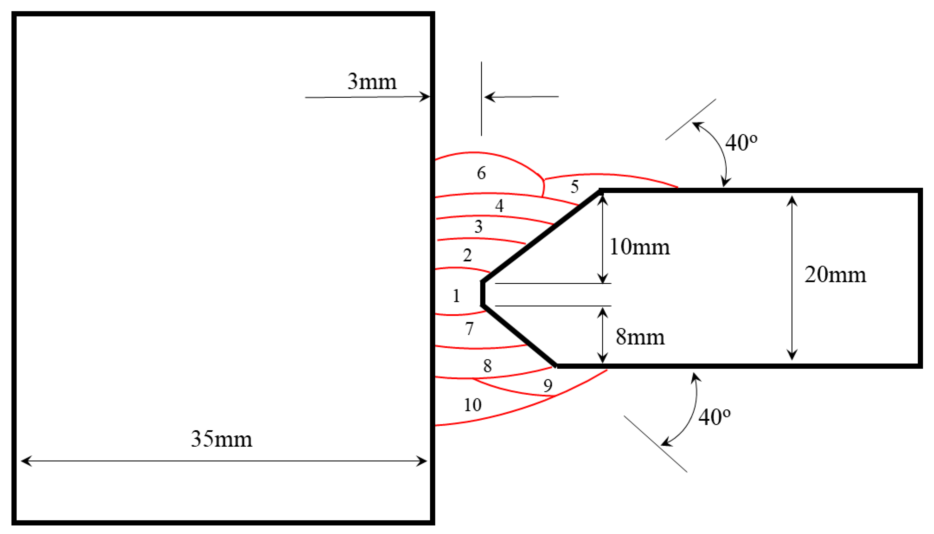
The base plate sample was 1000 mm long, 300 mm in width, and 35 mm thick. The web (stiffener) was 1000 mm long, 226 mm wide, and 20 mm thick. The web was welded onto the base plate with a weld length of 800 mm. Figure 1 shows a cross-section in the T-joint, which was used as a basis for the analysis.

2.2. Welding Procedure

The weld contained a sequence of ten passes, as shown in Figure 1. The first pass was done by a shielded metal arc with filler material (E20 18-M2) of 3.2-inch diameter. The remainder of the passes were done by submerged arc welding with filler material (ER-1205-1) brand L-Tec 120 of 3.2-inch diameter. The average heat input was 1.77 kJ/mm, and the welding speed for the first pass was 100 mm/min, and for all other passes was 150 mm/min. Also, preheat and interpass temperatures were 140 °C and 146 °C, respectively. The weld efficiency was assumed to be 75%.

2.3. Material Properties

The parent steel was BIS 812 EMA (equivalent to ASTM A514 Class F). It is a low alloy, quenched and tempered, high-strength steel. The steel was spray quenched from 950 °C and tempered at 590 °C.

Table 1. BIS 812 EMA Steel composition (wt%) [14].

C	Si	Mn	P	S	Cr	Ni	Mo	V
0.13	0.24	0.93	0.01	0.002	0.48	1.28	0.39	0.02
Ti	Cu	Al	Nb	B	Ca	O	Fe
0.01	0.21	0.07	0.01	0.0066	23 ppm	0.009	Bal

and

Table 2. Filler material composition (wt%) [14].

C	Si	Mn	P	S	Cr	Ni	Mo
0.08	0.34	1.74	0.009	0.004	0.31	2.72	0.62
V	Ti	Cu	Al	Nb	Ca	Fe
<0.01	0.01	0.02	<0.01	0.0081	<3 ppm	Bal

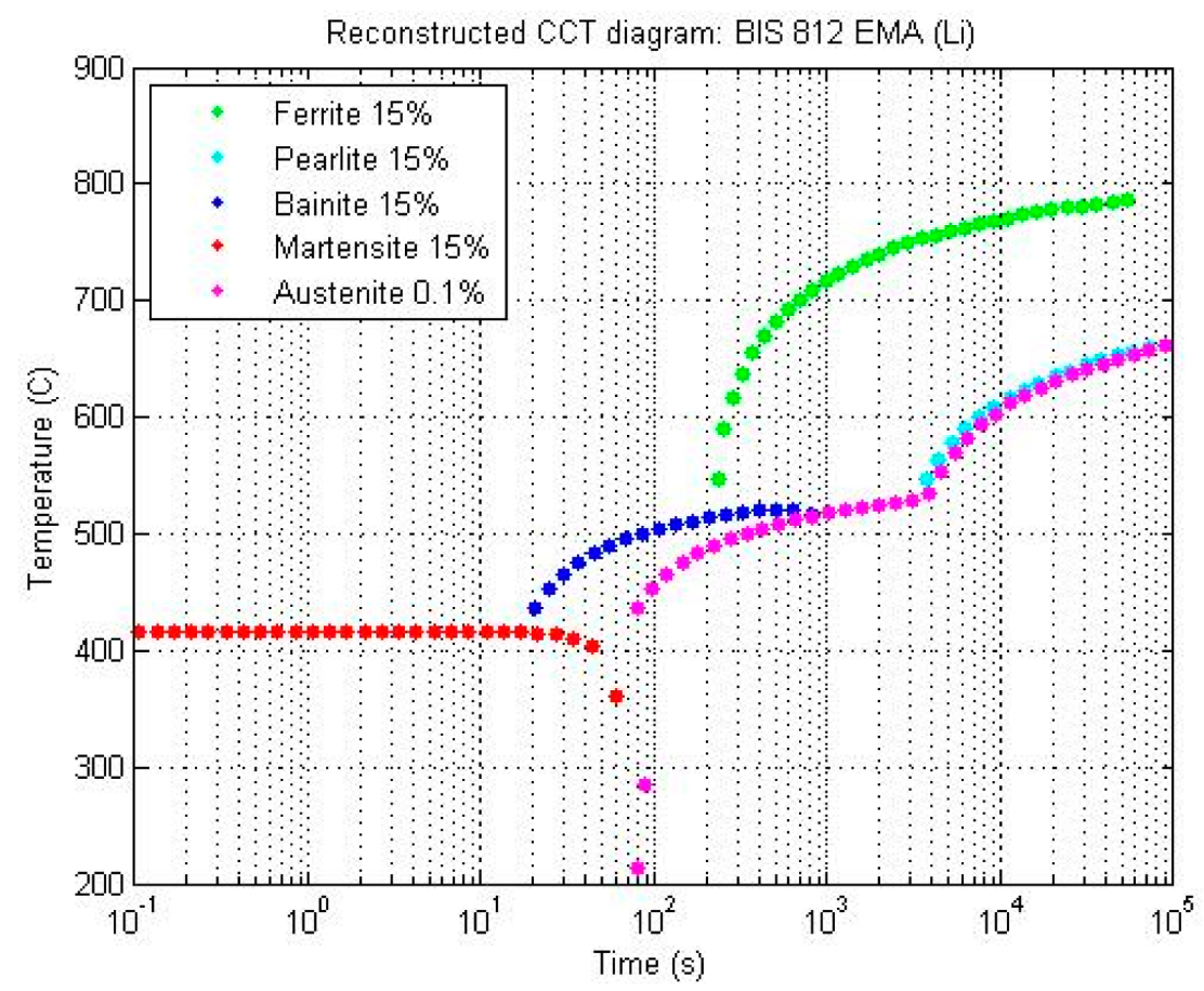
show the composition of both parent and filler materials. Figure 2 shows a continuous cooling transformation (CCT) diagram of the BIS 812 EMA, created from a composition-based model by Li [13].

Table 3. Thermal and mechanical properties of the parent steel.

Thermal Conductivity (W/m °C)	Temperature (°C)	Elastic Modulus (MPa)	Temperature (°C)	Yield Stress (MPa)	Temperature (°C)	Plastic Strain
35	20	214,000	20	458	20	0
37	200	130,000	800	711	20	0.1
26	800	10,700	1000	399	200	0
14	1480	2140	1480	620	200	0.1
14	1530	2140	1530	265	600	0
Expansion Coefficient (1/°C)	Temperature (°C)	Specific Heat (kJ/kg °C)	Temperature (°C)	37	800	0
1.16 × 10−5	20	460	20	57	800	0.1
1.36 × 10−5	400	595	375	4.58	1480	0
1.46 × 10−5	800	737	575	4.58	1480	0.1
1.52 × 10−5	1480	900	735	4.58	1530	0
1.52 × 10−5	1530	658	870	4.58	1530	0.1
		811	1480

Density 7.84 × 10⁻⁶ (Kg/mm³). Poisson’s ratio 0.3.

lists the thermal and mechanical properties of the parent steel.

3. Finite Element Modeling

This section describes the development of the finite element model and the procedure followed to set the input data, such as boundary conditions, heat source (loads), phase transformation, and bead deposition.

3.1. Finite Element Model

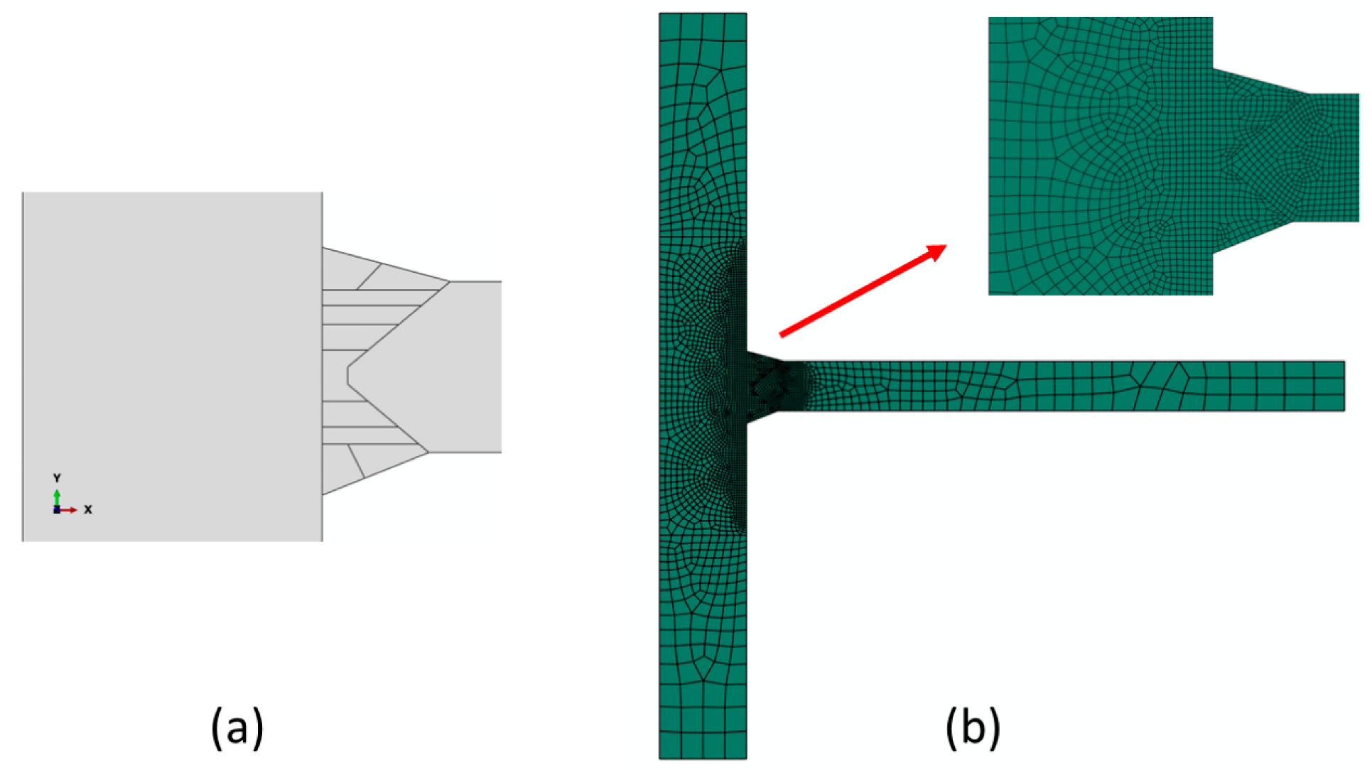
A two-dimensional thermo-mechanical, generalized plane strain finite element model was created to simulate the effect of phase transformation on residual stress during multi-pass welding in a thick section T-joint. Figure 3a,b show details of the weld beads and FE mesh of the T-joint model, respectively. The model consisted of 2906 quadratic elements and 14,854 nodes with 29,871 degrees of freedom (temperatures and displacements). All FE analyses were carried out using ABAQUS software [15]. Since ABAQUS does not have the capability to simulate the solid-state phase transformation, a user material (UMAT) subroutine was employed. This subroutine, which was developed by the research team in the school of materials at the University of Manchester [14], utilized the approach proposed by Leblond and Devaux [16] to take into account the metallurgical, and metal dilution effects.

Leblond’s model is expressed as follows:

$$\frac{d{P}_j\left(T\right)}{dt}=f\left(\dot{T}\right)·\frac{P_{j,eq}^{ij}\left(T\right)-P_j\left(T\right)}{{\tau }^{ij}\left(T\right)}$$

where $d{P}_j$ denotes the proportion per unit volume of phase j, and $P_{j,eq}^{ij}$ is the equilibrium proportion for phase j and ${\tau }^{ij}$ is time constants for the transformation i to j. All model parameters vary linearly between the start and finish temperatures of the phase transformations, which are listed in

Table 4. Start and finish temperatures of the phase transformations.

Phase	Start Temperature °C	Finish Temperature °C
Ferrite	800	600
Bainite	600	450
Martensite	400	200
Austenite	730	840

. The time constants ${\tau }^{ij}$ can be estimated simply as the time required to complete the transformation read from the continuous cooling transformation (CCT) diagram. The constants are given in

Table 5. Time constants used in the phase transformation.

Phase Transformation		$\mathbf{Start}{\mathit{\tau }}^{\mathit{i}\mathit{j}}$	$\mathbf{Finish}{\mathit{\tau }}^{\mathit{i}\mathit{j}}$
From (i)	To (j)	(Sec)	(Sec)
Austenite	Ferrite	500	500
Austenite	Bainite	9	90
Austenite	Martensite	0.2	2
Ferrite	Austenite	1	0.2
Bainite	Austenite	1	0.2
Martensite	Austenite	1	0.2

. The heating transformations from ferrite, bainite, and martensite to austenite are all assumed to be identical.

In the current study, volumetric strains were calculated from the coefficient of expansion and then an additional initial strain was imposed to represent a 3% reduction in volume on transformation to austenite and a 3% expansion on transformation from austenite. The formula for the additional initial strain is therefore expressed as follows:

$${\epsilon }_{ij}=0.01\cdot {\delta }_{ij}\left(p_4|{}_{t=0}-p_4\right)$$

where $p_4|{}_{t=0}$ is the initial austenite proportion, set to unity for each new bead and zero for the parent plate. The initial composition of the parent material is 60% ferrite and 40% bainite.

The effect of transformation plasticity was not included in the subroutine. Instead, the effect was approximated by supplying a separate temperature-dependent yield stress, as shown in Table 3.

The solid-state phase transformations occurred in the fusion zone (FZ) and heat-affected zone (HAZ). From the CCT diagram in Figure 2, the HAZ can be defined as the non-melted portion of the metal plate or solidified weld beads that were exposed to a temperature higher than 800 °C during welding process.

3.2. Loads

The thermal loads of the welding process were simulated as a body heat flux (Q_W) which can be calculated for each bead as follow:

$$Q_W=\frac{Q_J}{t}$$

(1)

where Q_J and t are the total energy per unit volume and the effective time for the torch to pass the bead, respectively. Q_J can be calculated using the following equation:

$$Q_J=\eta \frac{H}{A}$$

(2)

where, $\eta$ is the weld efficiency, which is assumed to be 0.75. A is the bead area and H is the heat input, which can be calculated as follows:

$$H=\frac{U\ast I}{v}$$

(3)

where U, I, and v are voltage, current, and welding speed.

The effective time for the torch to pass the bead (t) can be calculated as follows:

$$t=\frac{L}{v}$$

(4)

where L is the weld pool length, which is assumed to be 15 mm, and the welding speed (v) for the first pass is 100 mm/min, whereas the rest have a faster speed of 150 mm/min.

Table 6. Body heat flux parameters for each weld bead.

Pass No.	Bead Area (mm2)	Time (Sec)	Arc Efficiency	QJ (J/mm3)	QW (W/mm3)
1	22	9	0.75	60.34	6.7
2	21.5	6	0.75	61.74	10.29
3	22	6	0.75	60.34	10.06
4	22.5	6	0.75	59	9.83
5	21.5	6	0.75	61.74	10.29
6	21.5	6	0.75	61.74	10.29
7	21.5	6	0.75	61.74	10.29
8	20	6	0.75	66.38	11.06
9	22	6	0.75	60.34	10.06
10	21	6	0.75	63.21	10.54

contains all required parameters for body heat flux calculations for each weld bead.

3.3. Heat Source Model

Modelling of the heat source may be considered the key factor in any welding simulation. The ramp heat input function model, which is based on the disk model, has been used for this project for three main reasons. Firstly, to avoid the numerical divergence resulting from the rapid change in temperature around the fusion zone [17]. Secondly, for the ability to apply this model to 2D analysis. Finally, to simulate the effect of the moving heat source [18]. The arc energy has to be distributed with regard to torch travelling speed and welding pool length.

3.4. Boundary Conditions

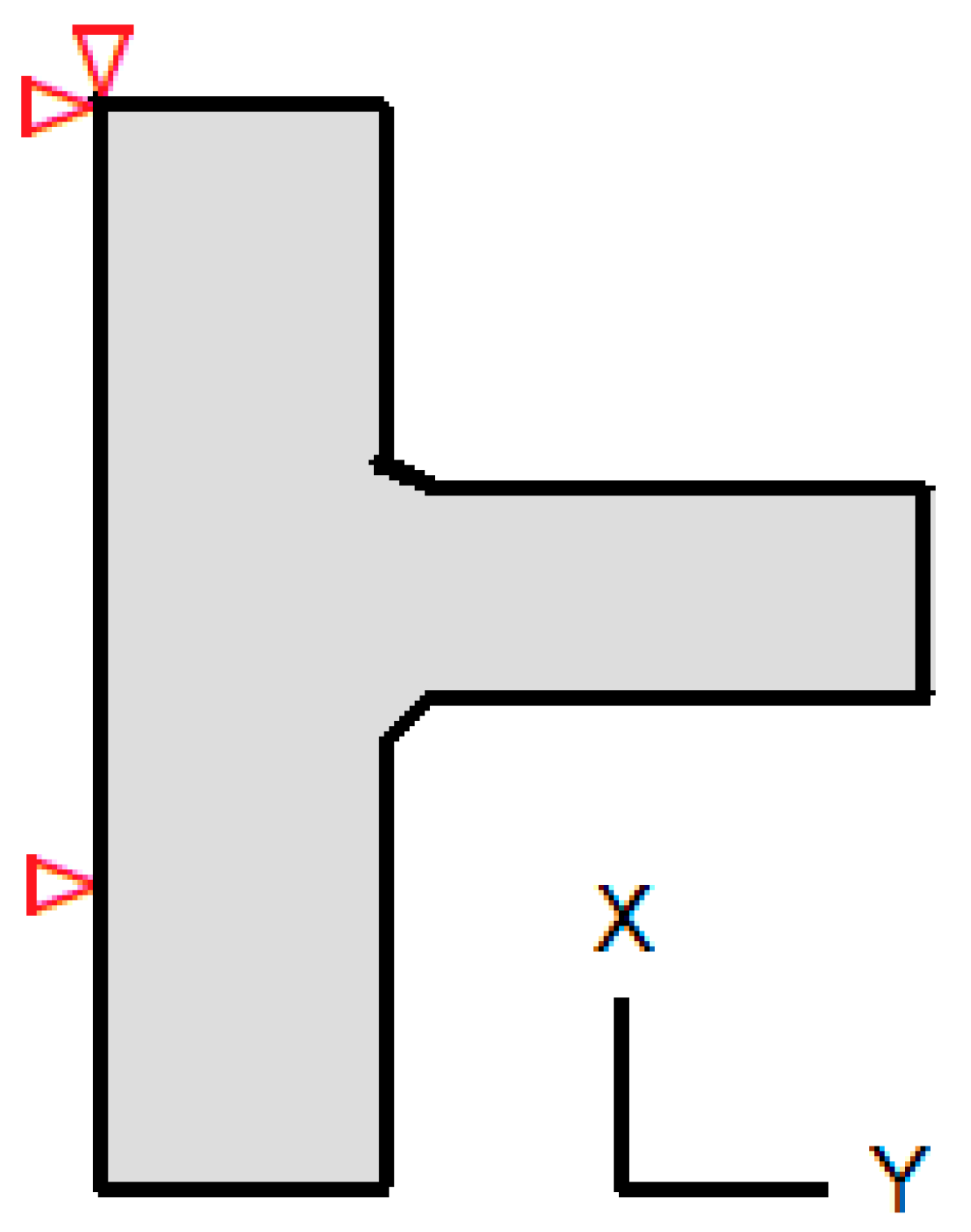
In the current T-joint model, there are mechanical and thermal boundary conditions. The mechanical boundary conditions prevent the structure from moving and rotating. The thermal boundary conditions account for the heat losses from the steel to the ambient environment via convection and radiation. Figure 4 illustrates the mechanical boundary conditions where two points have been selected to fix the model. The top node fixes the model in the X and Y directions while the bottom one restricts the body from rotation. This boundary condition represents a structure that is freestanding and not clamped.

The thermal boundary conditions enhance the model’s accuracy by considering the heat losses from steel plates to the ambient environment. Overall, convection has the dominant effect on heat transfer to the ambient environment. However, the radiation may only have a more significant effect in the melting pool [19]. Convection and radiation were applied to the whole web, the whole flange, and top beads from each weld side, which are beads 5, 6, 9, and 10, as shown in Figure 1.

Table 7. The convection and radiation heat transfer parameters.

Parameter	Value
Film Coefficiente	1 × 10−5 W/m2 K
Emissivity	0.4
Ambient temperature	20 °C
Boltzmann’s constant	5.669 × 10−14 W m2 K4
Absolute zero temperature	−273.15 °C

lists the convection and radiation heat transfer parameters.

4. Results and Discussion

4.1. Model Validation

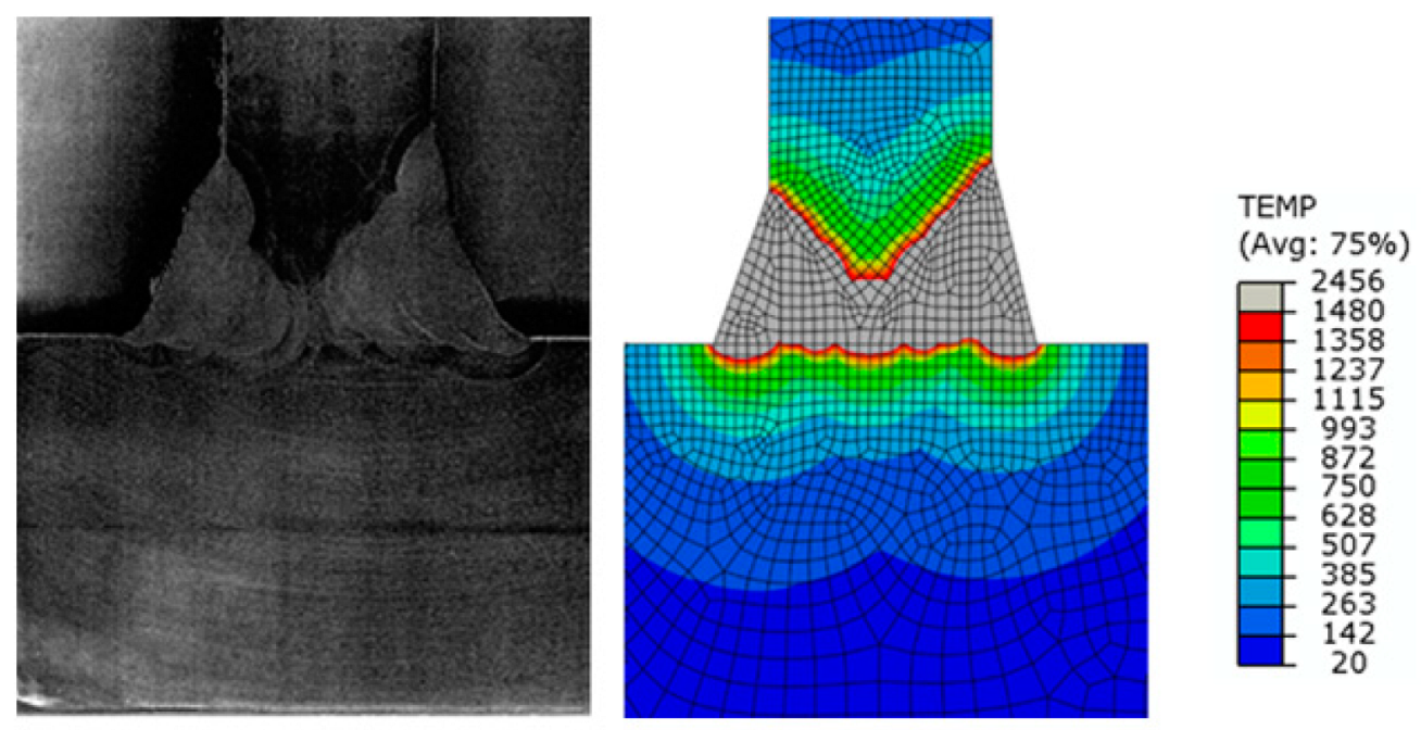
Heat source modeling is a critical component of any welding simulation. Three primary standards can be used to validate the model’s heat source accuracy. These standards include the peak temperature, shape, and size of the fusion zone [1]. A lot of efforts have been made to obtain the proper fusion boundary. Several factors were changed several times to get the right shape and size for the fusion zone, such as mesh size and bead geometry and size. Figure 5 shows good agreement between the fusion boundary in the weld macrograph and the FE model, which is represented by the gray color.

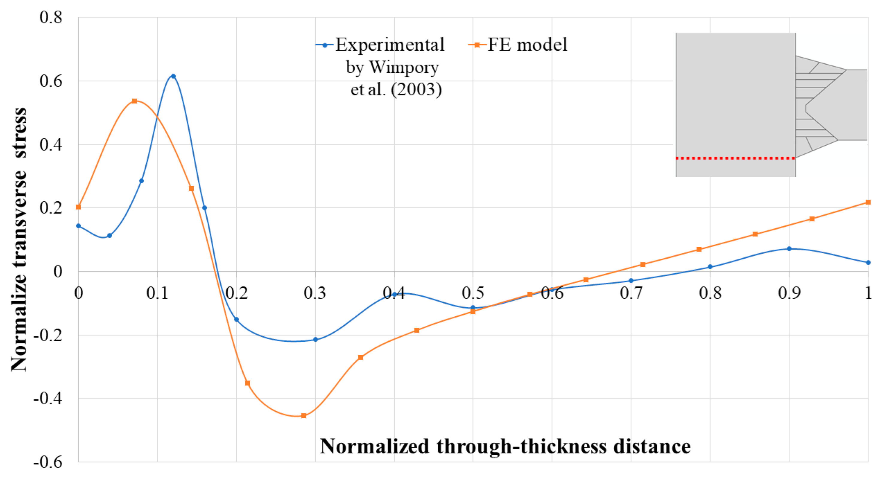
The experiment-based study conducted by Wimpory and his colleagues [20] was also used to validate the FE model developed in the present study. Wimpory used the deep-hole drilling method to measure the residual stress on a line through the plate thickness from the weld toe, as shown in Figure 6 (dashed red line). The comparison shows a good agreement in the behavior, but the values are slightly shifted. This may result from the different welding sequences between the experimental and FE modeling.

4.2. Effect of Phase Transformation and Martensite Start Temperatures

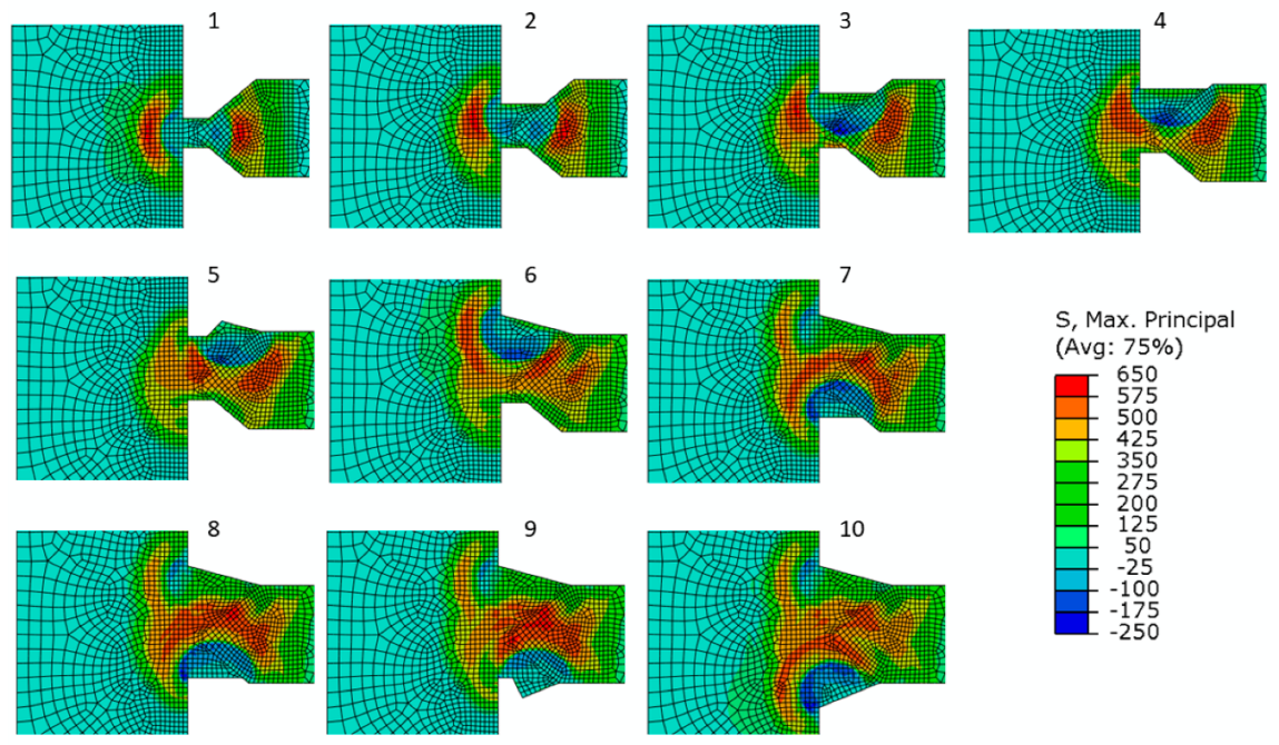
Figure 7 shows residual stress development in the FE model with Ms = 400 °C. It can be seen from the plot that phase transformation generated compressive residual stress underneath the bead to be deposited. Also, it provided a higher amount of tensile residual stress underneath the compression spot. The tensile residual stress was building continuously as more weld beads were deposited. The final distribution of residual stress shows compressive residual stress in and around the last bead to be deposited while the rest of the weld area was affected by tensile residual stress, which concentrated in the middle of the weld and in the flange along the underside of the weld. These stresses might lead to fatigue failure if there were interior voids or a lack of fusion in the internal beads.

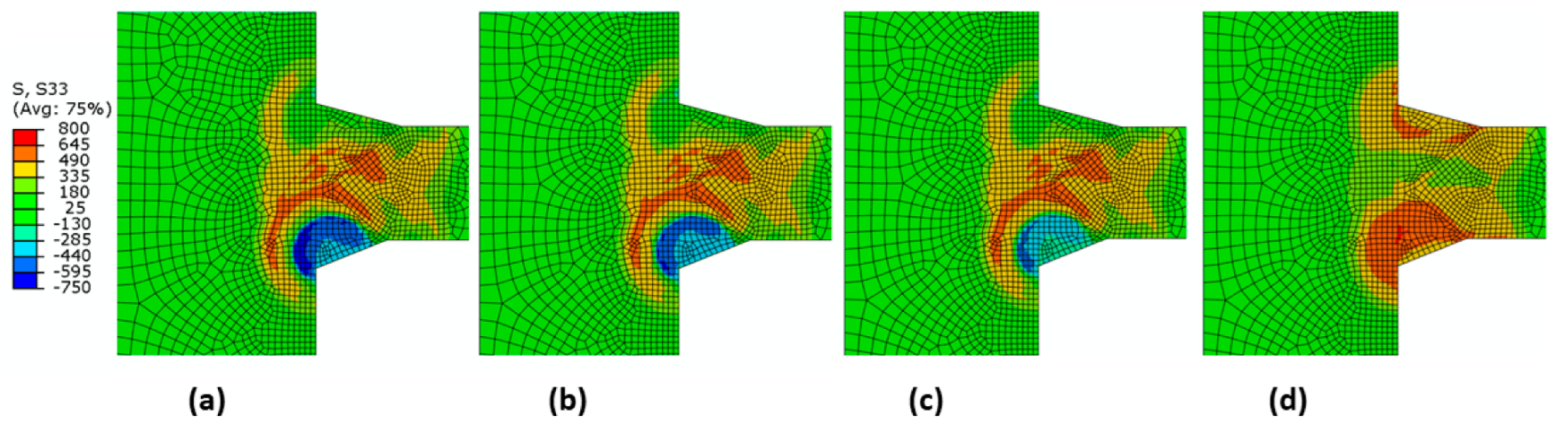
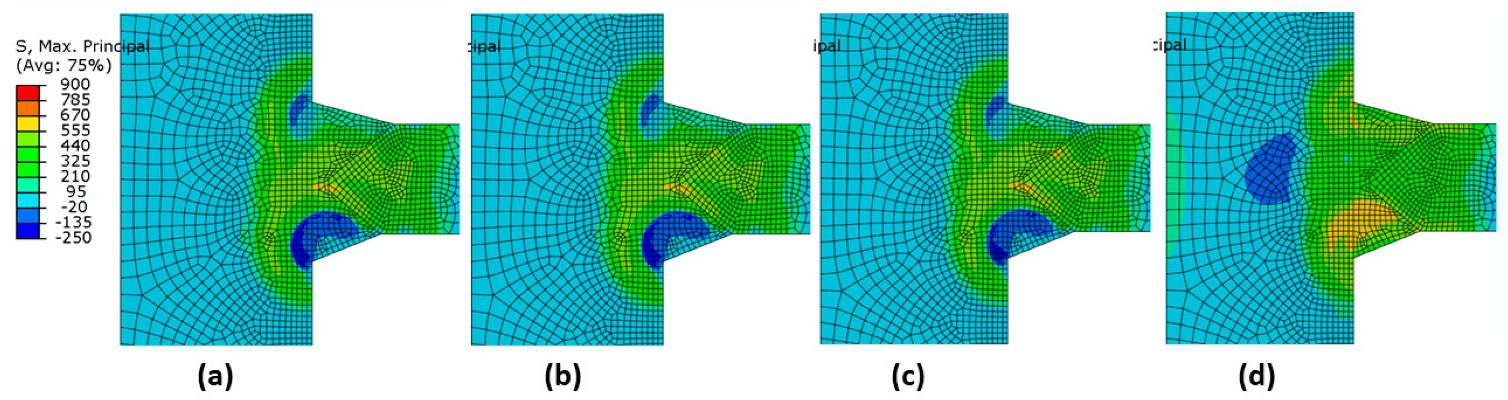
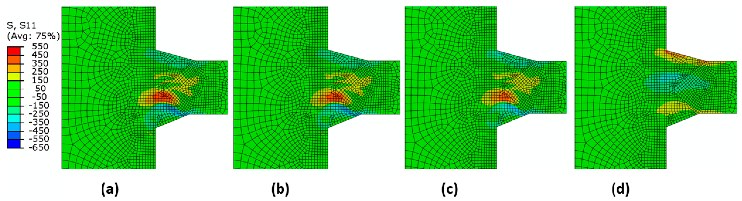
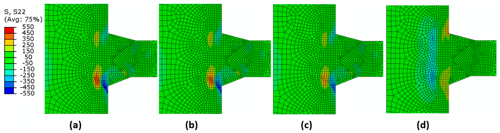
Figure 8, Figure 9, Figure 10 and Figure 11 compare the normal, transverse, longitudinal, and maximum principal stresses under four conditions: at Ms = 300, 350, 400 °C, and with no phase transformation. The model without phase transformation appears to give better results than the rest. It shows compressive stress normal to the plate in the weld area. Tensile stress in this direction could cause the growth of cracks existing from lack of fusion.

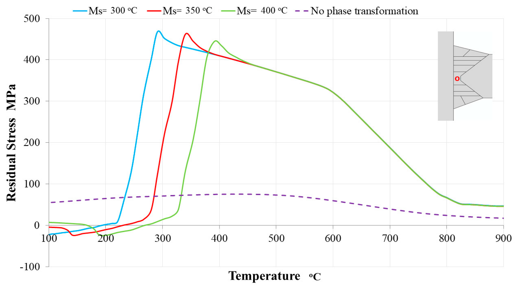
Two points have been selected from the fusion zone of the first and last beads to study the effect of both phase transformation and martensite start temperature (Ms) on the accumulation of residual stress during the cooling of the weld bead. Figure 12 and Figure 13 show residual stress accumulation in these two points under four different conditions, one without phase transformation and the rest taking into account phase transformation at different martensite start temperatures, which are 400, 350, and 300 °C.

In the first bead, Figure 12, phase transformation showed an insignificant effect on the final residual stress, whereas the martensite start temperature had an almost negligible effect. This is because both web and flange were free (not connected yet), and therefore, there was no restriction against the volume expansion during phase change. The residual stress values were 55 MPa in the model without phase transformation, 8 MPa in the model with Ms temperature 400 °C, −4 MPa in the model with Ms temperature 350 °C, and −22 MPa in the model with Ms temperature 300 °C. 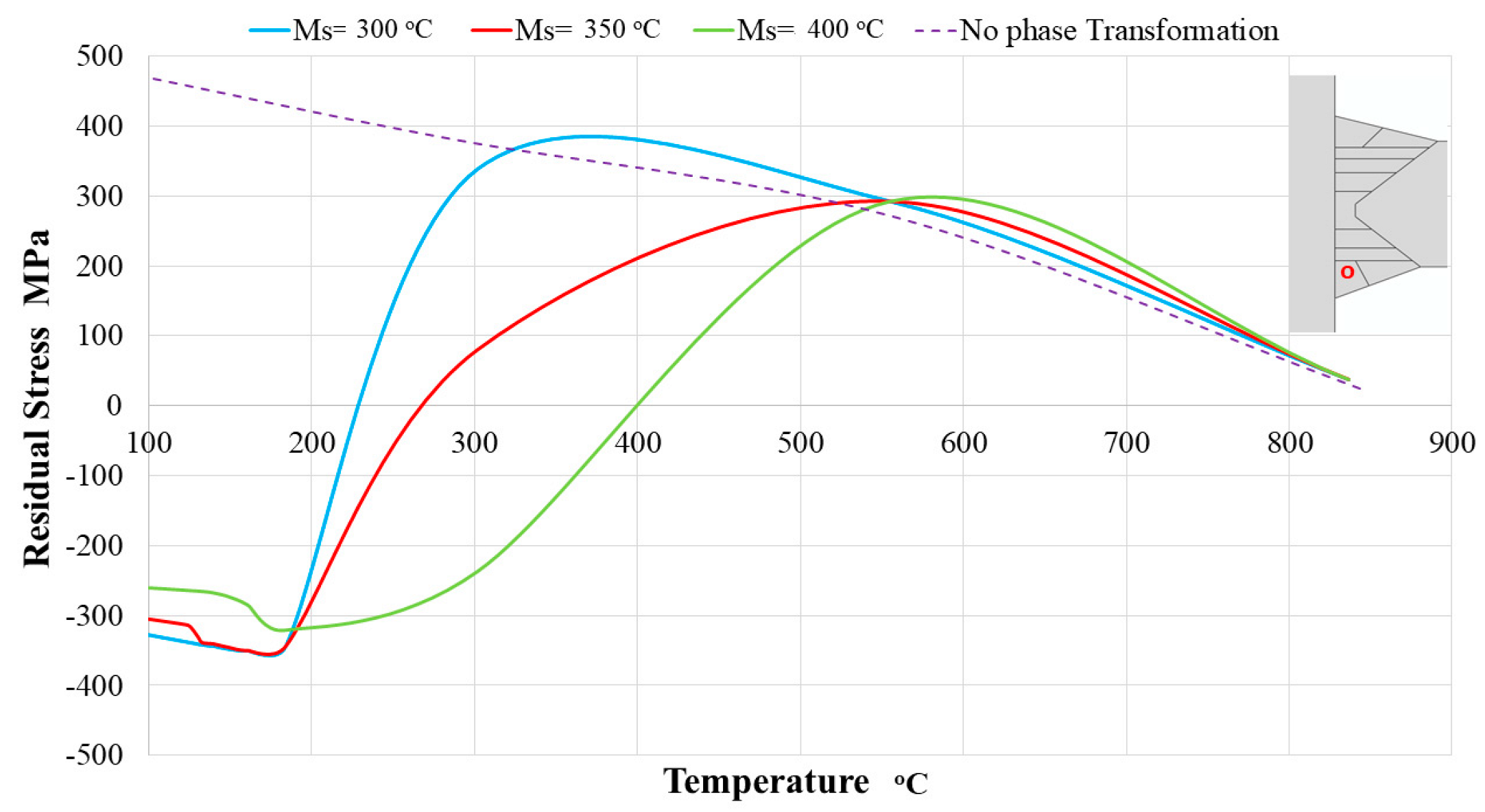In contrast, the phase transformation in the last bead made a massive difference, as shown in Figure 13. When the phase transformation was not included, it was observed that the tensile residual stress built up continuously until it peaked at 470 MPa at the end of the cooling process (interpass temperature). On the other hand, when the transformation was included, the tensile residual stress accumulated until it reached the martensite start temperature. Then, it decreased sharply before it started to build up again after the transformation was exhausted. The most significant compressive residual stress was produced in the model with a lower martensite start temperature. It can be seen from the graph that as the Ms temperature decreased, the compression stress increased. The values of the compressive residual stress in the model with Ms temperatures 400, 350, and 300 °C were found to be 260, 305, and 327 MPa, respectively. However, after a specific Ms temperature, the amount of compressive stress may not have increased with the reduction of Ms temperature. This can be observed when the martensite start temperature was changed from 350 °C to 300 °C. Both Ms temperature and the provided compressive stresses were nearly equal.

5. Conclusions

Various non-linear finite element simulations were carried out to understand the effect of phase transformation and martensite start temperature on the residual stresses in a multi-pass welded T-joint. Heat input and bead geometry were adjusted to provide realistic fusion boundaries for each bead as it was deposited, and the effect of re-melting was examined. In addition, two FE models were carried out, with and without phase transformation. Also, the martensite start temperature was changed several times to demonstrate its effect on residual stress accumulation. Finally, the results were compared to published experimental works to validate the FE model.

From the output results, it was found that, for this multi-pass weld model, phase transformation generated compressive residual stress underneath the last bead to be deposited. However, some restrictions around the bead were essential to provide that stress. Tensile residual stress was generated in the bulk of the weld area when phase transformation was considered. From that, it can be concluded that phase transformation may be useful for single pass and other groove welds but may be unhelpful in the case of the T-joint examined here. The martensite start temperature had an effect, but this was small compared with the main difference between having a phase transformation and not having one.

References

- Goldak, J.; Akhlaghi, M. Computational Welding Mechanics. In Encyclopedia of Thermal Stresses; Springer: Dordrecht, The Netherlands, 2014. [Google Scholar]
- Masubuchi, K. Analysis of Welded Structures, 1st ed.; Elsevier: Amsterdam, The Netherlands, 1980. [Google Scholar]
- Callister, W.D., Jr.; Rethwisch, D.G. Materials Science and Engineering; John Wiley & Sons: Hoboken, NJ, USA, 2020. [Google Scholar]
- Becker, M.; Jordan, C.; Lachhander, S.; Mengel, A.; Renauld, M. Prediction and Measurement of Phase Transformations, Phase-Dependent Properties and Residual Stresses in Steels; KAPL: Niskayuna, NY, USA, 2005. [Google Scholar]
- Ohta, A.; Matsuoka, K.; Nguyen, N.T.; Maeda, Y.; Suzuki, N. Fatigue Strength Improvement of Lap Joints of Thin Steel Plate Using Low-Transformation-Temperature Welding Wire. Weld. J. 2003, 82, 78-S. [Google Scholar]
- Ota, A.; Shiga, C.; Maeda, Y.; Suzuki, N.; Watanabe, O.; Kubo, T.; Matsuoka, K.; Nishijima, S. Fatigue strength improvement of box-welded joints using low transformation temperature welding material. Weld. Int. 2000, 14, 801–805. [Google Scholar] [CrossRef]
- Jones, W.K.C.; Alberry, P.J. A Model for Stress Accumulation in Steels during Welding. Met. Technol. 1977, 11, 557–566. [Google Scholar]
- Taraphdar, P.K.; Kumar, R.; Pandey, C.; Mahapatra, M.M. Significance of finite element models and solid-state phase transformation on the evaluation of weld induced residual stresses. Met. Mater. Int. 2021, 27, 3478–3492. [Google Scholar] [CrossRef]
- Deng, D.; Murakawa, H.; Liang, W. Numerical and experimental investigations on welding residual stress in multi-pass butt-welded austenitic stainless steel pipe. Comput. Mater. Sci. 2008, 42, 234–244. [Google Scholar] [CrossRef]
- Liu, C.; Zhang, J.; Xue, C. Numerical investigation on residual stress distribution and evolution during multipass narrow gap welding of thick-walled stainless steel pipes. Fusion Eng. Des. 2011, 86, 288–295. [Google Scholar] [CrossRef]
- Sattari-Far, I.; Farahani, M. Effect of the weld groove shape and pass number on residual stresses in butt-welded pipes. Int. J. Press. Vessel. Pip. 2009, 86, 723–731. [Google Scholar] [CrossRef]
- Giri, A.; Mahapatra, M.M.; Sharma, K.; Singh, P.K. A study on the effect of weld groove designs on residual stresses in SS 304LN thick multipass pipe welds. Int. J. Steel Struct. 2017, 17, 65–75. [Google Scholar] [CrossRef]
- Li, M.V.; Niebuhr, D.V.; Meekisho, L.L.; Atteridge, D.G. A computational model for the prediction of steel hardenability. Met. Mater. Trans. A 1998, 29, 661–672. [Google Scholar] [CrossRef]
- Keavey, M. Basic Thermal Diffusion with Phase Transformation & Dilatation. 2010; Unpublished report. [Google Scholar]
- Dassault Systemes Simulia Corp, Abaqus; Version 6.14; Dassault Systemes Simulia Corp: Providence, RI, USA, 2015.
- Leblond, J.; Devaux, J. A new kinetic model for anisothermal metallurgical transformations in steels including effect of austenite grain size. Acta Met. 1984, 32, 137–146. [Google Scholar] [CrossRef]
- Troive, L.; Jonsson, M. Numerical and experimental study of residual deformations due to double-J multi-pass butt-welding of a pipe-flange joint. Presented at the International Conference on Industry, Engineering, and Management Systems IEMS 1994, Cocoa Beach, FL, USA, 1994. [Google Scholar]
- Jiang, W.; Yahiaoui, K.; Hall, F.R.; Laoui, T. Finite Element Simulation of Multipass Welding: Full Three-Dimensional Versus Generalized Plane Strain or Axisymmetric Models. J. Strain Anal. Eng. Des. 2005, 40, 587–597. [Google Scholar] [CrossRef]
- Francis, J.D. Welding Simulations of Aluminum Alloy Joints by Finite Element Analysis. Int. J. Mag. Eng. Technol. Manag. Res. 2015, 2, 446–450. [Google Scholar]
- Wimpory, R.C.; May, P.S.; O’Dowd, N.P.; Webster, G.A.; Smith, D.J.; Kingston, E. Measurement of residual stresses in T-plate weldments. J. Strain Anal. Eng. Des. 2003, 38, 349–365. [Google Scholar] [CrossRef]
Figure 1.
Plate dimensions and weld sequence.
Figure 2.
CCT diagram for BIS 812 EMA steel [
14].
Figure 3.
Illustration of T-joint model, showing: (a) weld beads details in FE model; (b) FE mesh.
Figure 4.
Mechanical boundary conditions.
Figure 5.
Fusion boundary in real weld macrograph and FE model.
Figure 6.
Comparison between experimental and FE results.
Figure 7.
Residual stress development in the FE model with Ms = 400 °C.
Figure 8.
Normal residual stress in the FE model in different cases (MPa), (a) Ms = 300 °C, (b) Ms = 350 °C, (c) Ms = 400 °C, and (d) no phase transformation.
Figure 9.
Transverse residual stress in the FE model under different conditions (MPa), (a) Ms = 300 °C, (b) Ms = 350 °C, (c) Ms = 400 °C, and (d) no phase transformation.
Figure 10.
Longitudinal residual stress in the FE model under different conditions (MPa), (a) Ms = 300 °C, (b) Ms = 350 °C, (c) Ms = 400 °C, and (d) no phase transformation.
Figure 11.
Max. Principal residual stress in the FE model under different conditions (MPa), (a) Ms = 300 °C, (b) Ms = 350 °C, (c) Ms = 400 °C, and (d) no phase transformation.
Figure 12.
Stress accumulation at the 1st bead.
Figure 13.
Stress accumulation at the last (10th) bead.