Abstract
The hydraulic properties of fractures are greatly affected by the stress. Knowing the fluid flow behavior of fractures is of great importance to underground engineering construction and environmental safety. The main purpose of this paper is to study the fluid flow characteristics of rough fractures under different stress states. First, rough fracture surfaces were generated by using the corrected successive random addition (SRA) algorithm. Then, the sheared fracture models subjected to different stress condition were obtained under the boundary condition of constant normal stiffness (CNS). Finally, the hydraulic characteristics of the three-dimensional rough rock fractures were analyzed by numerically solving the full Navier–Stokes equation. It has been found that (1) the aperture of fractures all obeys the Gaussian distribution. The dilatancy effect is gradually obvious and aperture becomes larger with the increase of shear displacement. (2) When the initial normal stress increases, the contact area of fracture becomes larger and the reverse flow can be observed around the contact area. (3) The relationship between hydraulic gradient and flowrate exhibits nonlinearity which can be described by the Forchheimer’s law. The linear coefficient a and the nonlinear coefficient b gradually decrease with the increase of shear displacement and finally stabilize. The values of a and b are reduced by 1–2 and 1–3 orders of magnitude respectively during the shear. The critical Reynolds number increases with the increase of shear displacement and decrease as the initial normal stress increases.
1. Introduction
There are a large number of fractures with different sizes and occurrences in natural rock masses. The permeability of the rock matrix is significantly smaller than that of the fracture and the fracture network usually provides the main channel for groundwater seepage. Studying the hydraulic characteristics of single rock fracture is the basis for understanding the seepage mechanism of three-dimensional fracture network. It is of great significance to the construction of major energy and environmental projects such as oil exploration, geothermal energy extraction, and carbon dioxide storage [1,2,3]. The fracture flow becomes very complicated due to many factors such as stress, fracture geometry, and temperature. Limited by the difficulty of theoretical research, the methods of numerical simulation and laboratory tests are usually used to explore the influence of various factors on the fracture flow.
Early studies of fracture flow usually simplified the fractures to a combination of upper and lower smooth parallel plates and the cubic law was adopted to describe the fluid flow. However, the parallel plate model is inadequate to describe the hydraulic behavior of natural rock fractures. The roughness of fracture may cause an error of 1–2 orders of magnitude between real flow and cubic law [4]. To consider the influence of fracture geometry on flow characteristics, many scholars have developed different modified cubic law to improve the applicability of the traditional one. This was achieved by considering the factors of aperture, roughness, and contact area. Lomize and Louis [5,6] analyzed the relationship between flow rate and aperture in natural fractures through experiments and pointed out that the index of aperture in cubic law is 3 under laminar flow and 1.5 under turbulent flow. Ge developed a modified model for impressible laminar flow in irregular fractures which explicitly incorporated the true aperture and tortuosity [7]. Barton [8] put forward an empirical formular between roughness coefficient, mechanical aperture, and hydraulic aperture, which be further applied to the cubic law, and finally the modified cubic law based on the roughness coefficient was obtained. Iwai [9] carried out a large number of experiments and first proposed that the roughness mainly affect the fracture flow through the contact rate of fracture surface. Zimmerman et al. [10] pointed out that the fracture permeability is not only affected by the contact area, but also by the contact shape. By introducing the area contact rate, a modified cubic law is obtained. Wang et al. proposed an empirical correction factor which comprehensively considered factors of inertia terms, roughness, and tortuosity and obtained a modified Local Cubic Law [11]. The cubic law assumes that the fracture flow is laminar. It is a simplified form of the N-S equations ignoring the nonlinear term. However, the flow velocity in natural rock fracture is not always small. When flow velocity is large which corresponding to a higher Reynolds number, a nonlinear phenomenon of flow will appear. The inertial effect of fracture flow usually increases with the complexity of the void space geometry [12,13,14,15,16,17]. The ignorance of inertial effects results in greatly deviations from the actual situation, which leads to the inability to describe the flow behavior in rock fractures well. It is necessary to adopt the full Navier–Stokes equations that reflect the real flow to describe the fluid flow through the rough fractures.
The water existed in the fractured rock mass has an important impact on the reduction of rock strength and the deformation of the fracture. Many studies on laboratory test and numerical simulations of coupled shear flow have been reported [3,18,19,20]. The shear behavior of rock fractures was traditionally carried out under the constant load boundary conditions. With this boundary condition, the normal stress acting on the sheared fracture remains constant and the fracture is allowed to deform freely. The constant load boundary condition widely used in the slope stability analysis. However, for deep underground projects and rock slopes reinforced with bolts, the normal stress imposed on the fracture surface changes with shear and the fracture dilatancy is constrained by the surrounding rock. At this time, the conventional constant normal load boundary is no longer applicable, and the constant normal stiffness boundary condition should be adopted [21,22]. The importance of constant normal stiffness boundary condition for the real simulation of the shear behavior of rock fractures has been emphasized by many scholars. Indraratna et al. [23] developed a shear test instrument of rock joint based on the condition of CNS and experimentally studied the shear behavior of rough fractures with different initial normal stress. The result revealed that the mechanical properties of rough fractures was greatly influenced by the initial normal stress and the roughness of fractures. In order to clarify the hydraulic coupling mechanism in rock fractures during shear process, it is necessary to carry out research on the hydraulic characteristics of rough fractures under CNS boundary condition.
Many existing studies on shear-flow test usually simplify the fracture morphology or assume that the sheared fracture is under constant load boundary. There are relatively few studies on the coupled shear flow in rough fractures with constant normal stiffness boundary. In this study, the self-affine rough fracture surfaces were produced with the application of corrected SRA algorithm. The influence of initial normal stress on the distribution of fracture aperture under the CNS condition was then analyzed. Based on the aperture distributions, the 3D fracture models were obtained. Finally, a number of numerical simulations were implemented to solve the nonlinear N-S equations of fluid in rough fractures. The nonlinear flow behaviors of rough fractures under the different stress state were analyzed in detail according to the relationship between flowrate and pressure gradient.
2. Generation of 3D Rough Fractures
2.1. Self-Affine Fracture Surfaces Based on Corrected SRA Algorithm
The natural rough rock fracture surface is rough and has fractal characteristics [24]. It is difficult to characterize the complex topography of the natural rough surface with a general function. Many studies have shown that it is reasonable to simulate the rough fracture surface with fractal geometry and the Fractional Brownian motion (FBm) which belongs to the self-affine fractal theory is considered the best fractal model to characterize the natural surface [25,26,27,28,29]. Due to the advantages of high efficiency and easy to understand, the SRA algorithm was employed to simulate fractal surface in this study.
In fBm, the random function z (x, y) with two independent variables (x, y) was adopted to characterize the undulation of the surface asperity. The increments of the random function over the interval h obeys a Gaussian distribution [5,30]. The random function of fBm is displayed as
In the above <·> represents the mathematical expectation, and H is the roughness exponent varying from 0 to 1, σ2 is the variance of random function.
In order to overcome the logical mistakes and questionable correlation associated with the conventional SRA algorithm, Liu et al. [31] developed a corrected SRA algorithm and verified its high efficiency and correctness through simulating the heterogeneity of subsurface. In this research, a number of rough fractures with different roughness exponent (H = 0.5, 0.55, 0.6) were generated by employing Liu’s algorithm. Figure 1 displays three fracture surfaces with a side length of 200 mm. It can be seen obviously that the height of surface asperity becomes smaller with the increase of roughness exponent.
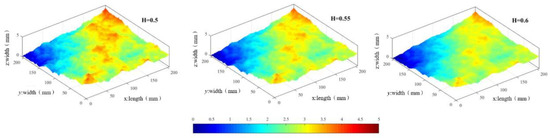
Figure 1.
Generated rough fracture surface.
The roughness of the fracture surface can be characterized by the cross-sectional profile parallel to the shear direction which is the suggested method by the International Society for Rock Mechanics and Rock Engineering (ISRM) to calculate the Joint Roughness Coefficient (JRC) of rough fracture (1981). In this study, 11 profiles alone with the shear direction (x direction) were selected and each profile was 10 mm apart alone the y direction. The following equations that proposed by Tse [32] was used to calculated the JRC values of fracture surfaces. The corresponding JRC values of H = 0.5, 0.55, 0.6 were 18.33, 12.45, 6.61.
where Δx is the interval, M is the number of intervals and zi is the height of surface asperity.
2.2. Aperture Distribution
The distribution of void spaces in natural fractures is anisotropic. The combined effect of geological history and stress field determines the geometry of the fracture aperture. Rock fractures may be subjected to shearing during their formation history, such as disturbances caused by earthquakes and excavations. The shear behavior will change the spatial geometry of fractures which result in anisotropy of the distribution of aperture.
The aperture plays a vital role on the hydraulic behavior of rock fractures. In this research, it is assumed that the upper and lower fracture surfaces are closed at the initial state. During the shearing process, the two fracture surfaces misaligned in the horizontal and vertical directions. The aperture can be calculated using the Equation (3) with a given shear displacement.
where z(x,y) is the height of surface asperity, uh is the shear displacement, uv is normal deformation during the shear.
Restricted by the laboratory test conditions, many studies of joint shear test were carried out under constant normal load boundary conditions. However, some scholars have emphasized that the constant normal load boundary condition is no longer applicable when the rock joints are constrained by surrounding rock mass and the application of constant normal stiffness condition is more appropriate in many engineering projects. In this research, the Equation (4) proposed by Indraratna et al. [23] was adopted to calculate the shear dilations under the constant normal stiffness conditions.
where uv is the shear dilation, is shear dilation rate and uh is the shear displacement under constant normal stiffness boundary conditions.
In Equation (4) the shear dilation rate always changes with the in which the uh-peak represents the peak shear displacement. The relationship between the shear dilation rate and is shown as
where is the peak dilation rate that can be obtained through Equation (6); and are decay constants which can be calculated from experimental data; for rough fractures it is usually assumed that the value of is 0.3 when the shear dilation appears.
Here, Kn is the constant normal stiffness imposed by the external environment. JRC is an exponent representing the roughness of fracture surface. M is the damage factor, and the values under high normal stress and low normal stress are 2 and 1 respectively. σn0 is the initial normal stress imposed on the rough fracture. JCS represents the compressive strength of fracture. kni is the initial normal stiffness without external constraint. Vm is the maximum closure value of fracture aperture. The related parameters for calculating the fracture aperture are listed in Table 1.

Table 1.
Related parameters for calculating fracture aperture.
High-precision solving the full Navier–Stokes equations of fluid flow in 3D rough fractures requires huge computational resources. Limited by this, only a part of squares on generated fracture surface was selected to form the 3D rough fracture model. The selected part is within the range of x = [100,130] mm, y = [40,70] mm with a side length of 30 mm.
This paper mainly investigated the flow characteristics of rough fractures under different stress states, without considering the influence of different roughness, so only the rough surface with H = 0.6 (corresponding JRC value is 6.61) was selected as the original fracture surface, which is corresponding to the fracture surface of fine sandstone in [23]. The distribution of aperture under different stress condition is shown in Figure 2. It can be found that the aperture of fractures all obey the Gaussian distribution. The value of aperture gradually decreases with the increase of initial normal stress under the same shear displacement. When the shear displacement is 4 mm, more places with the aperture of 0 value appeared as the initial normal stress increased, which indicated that the contact area is increasing. The aperture values become larger with the increasement of shear displacement, which is caused by the dilatancy effect. The increasement of shear displacement leads to the uneven body of fracture surface to slip and finally to be broken. The slip and damage of the uneven body result in irreversible dilatancy of the fracture surface.
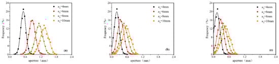
Figure 2.
Gaussian distribution of aperture, (a) σn0 = 0.4 MPa; (b) σn0 = 0.8 MPa; (c) σn0 = 1.6 MPa.
3. Numerical Simulation of Fluid Flow in Rough Fractures
3.1. Governing Equation of Fluid Flow
The Navier–Stokes equation describes the conservation of momentum of viscous incompressible fluids which can accurately reflects the basic mechanics of fluid flow. Equation (7) is the expression of Navier–Stokes equation for a single Newtonian fluid that is incompressible.
In the above, is the vector form of fluid flow velocity, represents kinematic viscosity of Newtonian fluid and can be expressed as , is the dynamic viscosity of the fluid. is the fluid density. is the fluid pressure, is the volume force.
The N-S equation is composed of multiple nonlinear partial differential equations. The left side of the equation reflect the effect of inertial force, where the convection term ((u▽)u) is the only nonlinear source of the equation, and the right side reflects the viscous force of the fluid. The N-S equations only has an analytical solution for very simple fluid flows. When solving complex problems, the numerical methods must be used. In order to accurately analyzed the fluid flow behavior in 3D rough rock fractures, the COMSOL Multiphysics software was adopted.
3.2. Boundary Conditions
The fluid is assumed to flow alone with the y direction with the inlet boundary of y = 0 mm and outlet boundary of y = 30 mm. The flow boundary conditions and pressure boundary conditions were implemented on the inlet and outlet, respectively. Five different flowrates were applied at the inlet.
4. Results and Analysis
4.1. Fluid Flow Behavior of Sheared Rough Fractures
In this study, the rough fracture with H = 0.6 was selected to form the three-dimensional rough fracture model and then the fluid flow behavior in fractures under different stress state was analyzed. The aperture of fractures presented an anisotropic distribution, which lead to the uneven distribution of the flow field. Figure 3 shows the cross-sectional view and arrow diagram of flow velocity in the y direction with which the shear displacement is 4 mm. Obviously, the distribution of flow velocity in rough fracture is inhomogeneous. The velocity range in the y direction in Figure 3e is about 6 times that in Figure 3a. The main reason of this phenomenon is that the aperture decreased with the increasement of initial normal stress and the contact of fracture surface increased the complexity of the flow field. With the same inlet flowrate, the flow velocity is larger in the fracture with smaller aperture. The contact area of fracture gradually increases with the increase of initial normal stress which lead to an anisotropic distribution of aperture. The fluid flow path become more tortuous and obvious preferential flow appears, which can be seen from Figure 3b,d,f.
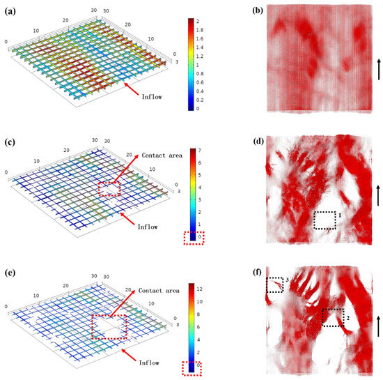
Figure 3.
Velocity in the y direction of the three-dimensional fracture model when the inlet flow rate was 1.443 × 10⁻⁵ m3/s, (a) σn0 = 0.4 MPa; (c) σn0 = 0.8 MPa; (e) σn0 = 1.6 MPa; (b,d,f) are the arrow diagrams of flow rate corresponding to (a,c,e) respectively.
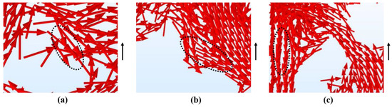
As shown in the flow field diagram, the low-velocity areas mainly locate near the contact area and the places with small aperture value. The negative value of uy can be seen from Figure 3c,e. The main reason for this phenomenon is that the low-velocity fluid located around the contact point was forced to flow around the contact area, and the flow has obvious tortuous effects. It can be seen from Figure 4 that the tortuous effects of the fluid around the contact area leads to scattered flow paths in the coordinate axis direction, which significantly increases the tortuous of the flow route, and even caused the fluid to flow in the negative direction of the y-axis.
Assuming that the fluid flows through the fracture at a sufficiently low flow rate, the N-S equation can be simplified to the form of the cubic law.
where μ is the dynamic viscosity of the fluid, w is the width of fracture, eh is the hydraulic aperture, is the pressure gradient, Q is the volume flowrate.
The cubic law can only be applied to the situation of low flow velocity due to the ignorance of inertial effect. At higher flow velocity, the flowrate (Q) and pressure gradient () has obviously deviated from the linear relationship. The Forchheimer equation is often used to describe the characteristics of nonlinear flow in fractures caused by inertial effects.
where, a is linear coefficients and b is nonlinear coefficients. The linear term (aQ) represents the effect of viscosity and the quadratic term (bQ2) represents the influence of inertial force.
Five boundary conditions of different flowrates were applied at the entrance of the fracture, and the relationship between the pressure gradient and the volume flowrate in the fracture under different stress state was obtained as shown in Figure 5. It can be seen that the Forchheimer equation can fit the data well. With the increase of initial normal stress, the curve of pressure gradient and flowrate becomes steeper, indicating that the flow resistance becomes larger. This is mainly because the larger the initial normal stress during the shearing process, the greater the amount of fracture closure caused and the fracture with higher initial normal stress required higher energy to reach the same flow velocity.
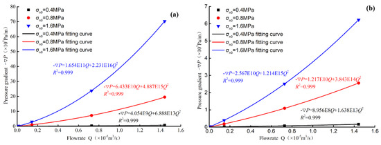
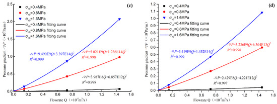
Figure 5.
Relationship between pressure gradient and flow rate under different initial normal stresses, (a) uh = 4 mm; (b) uh = 6 mm; (c) uh = 8 mm; (d) uh = 10 mm.
The linear and nonlinear coefficients in the Forchheimer equation under different stress state were obtained according to the fitting result. Figure 6a,b are the relationship curves of linear coefficient a, nonlinear coefficient b and shear displacement under different initial normal stresses. In the shearing process, the values of a and b were reduced by 1–2 and 1–3 orders of magnitude, respectively, and the value of the nonlinear coefficient b was 5 orders of magnitude larger than the value of the linear coefficient a. The changing trends of coefficients a and b were similar, falling rapidly in the interval of shear displacement of 4–6 mm, and gradually reach a stable state when the shear displacement exceeds 6 mm. The fracture expanded during the shearing process, and the hydraulic resistance formed on the fracture surface decreased, which lead to the decrease of a and b values. In addition, it can be observed that the values of the linear coefficient a and the nonlinear coefficient b increased with the increase of the initial normal stress. This is mainly due to the fact that the implement of higher normal stress makes it easier to inhibit the expansion of fracture and the contact area of the upper and lower fracture surfaces increased, which result in tortuous flow and inertial effects became obvious. At the same time, more broken particles will be produced under higher initial normal stress, which will hinder the fluid flow in the fractures. The relationship curve between linear coefficient a and nonlinear coefficient b is shown in Figure 7. The least squares method was used to fit the data, and the empirical formula between a and b was obtained as Equation (11). The value of the nonlinear coefficient b is often difficult to obtain in engineering practice. This equation can effectively estimate the nonlinear coefficient b according to the linear coefficient a.
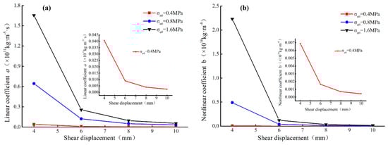
Figure 6.
Relationship between coefficients of Forchheimer equation and shear displacement under different initial normal stresses, (a) linear coefficient a; (b) nonlinear coefficient b.
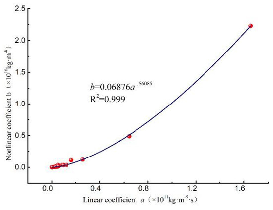
Figure 7.
Relationship between nonlinear coefficient b and linear coefficient a.
For fluid flow in rock fractures, with the increase of the flowrate in the entrance boundary, the nonlinear effect of the flow becomes more obvious. At this time, the inertial effect can no longer be ignored. It becomes the main cause of fluid energy loss. In order to quantitatively describe the nonlinear characteristics of the flow in the shearing process, the nonlinear factor E was defined, and its expression is
where the nonlinear factor is the ratio of the pressure drop caused by the non-linear effect to the total pressure drop. In engineering practice, it is generally believed that when E exceeds 0.1, the energy loss caused by nonlinear effects cannot be ignored. The E = 0.1 was selected as the turning point of the flow state. In order to quantitatively evaluate the starting conditions of nonlinear characteristics, the Reynolds number (Re) was introduced, and its expression is
Combining Equations (11) and (12), the critical Reynolds number Rec at the beginning of the nonlinear flow in the fracture can be derived, and the formula is
The values of a and b, which was calculated according to Forchheimer equation, were substituted into the Equation (12) to obtain the critical Reynolds number under different stress states. As shown in Table 2, the range of critical Reynolds number is between 20.95–166.28. It can be seen from Figure 8a that the critical Reynolds number increased with the increasing shear displacement, which is consistent with the experimental results of Yin’s [33]. Figure 8b is a comparison diagram of critical Reynolds number between our study and Yin’s with the initial normal stress of 0.8 MPa. The variation trend of the critical Reynolds number with the shear displacement is consistent with Yin’s, but the value is slightly larger than that of the literature, which is mainly caused by the difference of the fracture surface.
Table 2.
Corresponding a, b, and Rec values of rough fractures (H = 0.6) under different stress states.
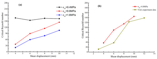
Figure 8.
Relationship between Reynolds number and shear displacement, (a) relationship between Reynolds number and shear displacement under different initial normal stress; (b) comparison of Reynolds number between simulation result and Yin’s experiment data [33].
4.2. Normalized Transmissivity
Transmissivity (T) is a parameter that comprehensively reflects the flow resistance existed in a fracture. When Re is sufficiently low, T is a constant value related to permeability and the Cross-sectional area of fluid flow. In this study, for fluid flow through sheared rough fractures subjected to different initial normal stress, the expression of T was shown as
where, ∇P is the pressure gradient alone the flow direction, MPa/m; Q is the flowrate in fracture, m3; μ is the dynamic viscosity, Pa·s.
Figure 9 displays the relationship between Reynolds number and transmissivity for sheared rough fractures under different initial normal stress ranging 0.4 to 1.6 MPa. Obviously, with the increase of Reynolds number, the values of transmissivity gradually decrease accompanied with the reduction of decrease rate. The relationship between Reynolds number and transmissivity can be best fitted with a second-polynomial function by using the least square method. The fitting relationships are presented in Figure 9.
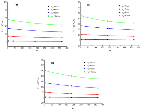
Figure 9.
Relationship between transmissivity and Reynolds number, (a) σn0 = 0.4 MPa; (b) σn0 = 0.8 MPa; (c) σn0 = 1.6 MPa.
The normalized transmissivity is defined as a dimensionless ratio of transmissivity(T) at a certain flow rate to transmissivity(T0) at a sufficiently low flowrate. It is more common to evaluate the nonlinear flow behavior of fluid using the relationship between Reynolds number and normalized transmissivity(T/T0). The T/T0 can be expressed as a function of Re and Forchheimer coefficient β [33]
where T0 is the transmissivity when the flowrate is significantly small and the values can be obtained from Figure 9. By fitting the data of T/T0 and Re in Figure 10 according to the Equation (15), the Forchheimer coefficient (β) can be obtained.
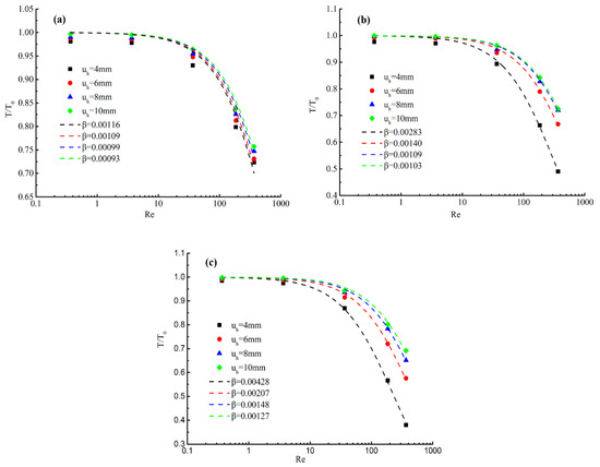
Figure 10.
Relationship between normalized transmissivity and Reynolds number, (a) σn0 = 0.4 MPa; (b) σn0 = 0.8 MPa; (c) σn0 = 1.6 MPa.
Figure 10 exhibits the relation between the Reynolds number and the normalized transmissivity of sheared fractures subjected to different initial normal stress. It can be seen from Figure 10 that the normalized transmissivity decreased a lot with increasing Reynolds numbers. For a certain initial normal stress, the relationship between Re and T/T0 shift upward as shear displacement increases. The reason is that the complexity of aperture geometry gradually weakens as the increase of shear displacement and the flow channel gradually increase as the decrease of contact ratio.
Figure 11 displays the relationship between Forchheimer coefficient and shear displacement. Notably, the Forchheimer coefficient decrease with the increase of shear displacement. Taking σn0 = 1.6 MPa as example, as the shear displacement increase from 4 mm to 6 mm, the Forchheimer coefficient decrease from 0.00428 to 0.00127 with reduction rate of 70.33%. While, with the same shear displacement, the Forchheimer coefficient generally increase with the initial normal stress.
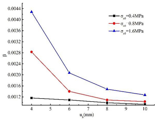
Figure 11.
Relationship curves of shear displacement (uh) and Forchheimer coefficient.
5. Conclusions
This paper numerically studied the effect of initial normal stress on variations in nonlinear flow through 3D self-affine rough fractures subjected to CNS boundary. First, several fracture surfaces with fractal properties were generated by using the corrected SRA algorithm. Then, the three-dimensional rock fracture under different stress states was developed, considering the boundary conditions of constant normal stiffness in the shearing process. Finally, the law of fluid flow in the fracture under different stress states was revealed by numerically solving the N-S equations corresponding to five different flowrate inlet boundary conditions. The aperture distribution, fluid flow pattern, critical Reynolds number and the normalized transmissivity of rough fractures were analyzed. The relevant results are summarized as follows:
- (1)
- With the increase of the initial normal stress during the shearing process, the surface contact area increases, and the average aperture value of the fracture decreases. The uneven body on the surface of the fracture gradually slipped with the increase of the shear displacement and was finally broken, resulting in a dilatancy effect. The fracture aperture has anisotropic characteristics under different stress state.
- (2)
- The larger the initial normal stress imposed on the external boundary, the stronger the unevenness of the flow field distribution. The negative value of the flow velocity appeared near the contact area of upper and lower fracture surfaces is mainly due to the obvious tortuous effect of the fracture flow, which leads to the scattered flow route and the reverse flow along the y-axis.
- (3)
- The Forchheimer equation can fit the data of the flowrate and pressure gradient well, which showed that the fracture flow no longer satisfies the law of linear flow. The linear coefficient a and the nonlinear coefficient b decrease with the increasing shear displacement, and increase when initial normal stress became larger. The values of a and b fall rapidly in the interval of shear displacement of 4–6 mm, and then reach a stable state. The empirical formula between the coefficient a and b was obtained by fitting all data points. By defining the nonlinear factor, the critical Reynolds number which is used to characterize the beginning of the non-linear flow was obtained.
- (4)
- The value of Re has significant effect on transmissivity and the transmissivity decrease with the increasing Re. The correlation between normalized transmissivity and Reynolds number were evaluated. The values of T/T0 increased with increasing uh but decrease with σn0. The values of β showed a decreasing trend with uh.
Author Contributions
Conceptualization, Q.G. and M.W.; Methodology, M.W., Q.G. and P.S.; Software, Q.G., Y.T. and B.D.; Validation, M.W., P.S. and Y.T.; Investigation, Q.G. and M.W.; Data curation, Q.G. and M.W.; Writing—original draft preparation, M.W. and P.S.; Writing—review and editing, Q.G., Y.T. and B.D.; Supervision, Q.G. and P.S.; Project administration, M.W., Q.G. and P.S.; Funding acquisition, Q.G., P.S. and B.D. All authors have read and agreed to the published version of the manuscript.
Funding
This work was supported by Open Fund of State Key Laboratory of Water Resource Protection and Utilization in Coal Mining (grant no. GJNY-18-73.11), the Key Laboratory of Western Mine Exploitation and Hazard Prevention, Ministry of Education (grant no. SKLCRKF1901), the Basic Research Fund of Central University (grant no. FRF-IDRY-20-032), the National Natural Science Foundation of China (grant no. 51804163).
Data Availability Statement
The data presented in this study are available upon reasonable request to the corresponding author.
Conflicts of Interest
The authors declare no conflict of interest.
References
- Zimmerman, R.; Bodvarsson, G. Hydraulic conductivity of rock fractures. Trans. Porous. Media 1996, 23, 1–30. [Google Scholar] [CrossRef] [Green Version]
- Berkowitz, B. Characterizing flow and transport in fractured geological media: A review. Adv. Water Resour. 2002, 25, 861–884. [Google Scholar] [CrossRef]
- Rong, G.; Yang, J.; Cheng, L.; Zhou, C. Laboratory investigation of nonlinear flow characteristics in rough fractures during shear process. J. Hydrol. 2016, 541, 1385–1394. [Google Scholar] [CrossRef]
- Tsang, Y. The effect of tortuosity on fluid flow through a single fracture. Water Resour. Res. 1984, 20, 1209–1215. [Google Scholar] [CrossRef]
- Lomize, G. Flow in Fractured Rocks; Gosenergoizdat: Moscow, Russia, 1951; Volume 127, p. 635. [Google Scholar]
- Louis, C. Rock Hydraulics in Rock Mechanics; Muller, L., Ed.; Verlay Wien: New York, NY, USA, 1974. [Google Scholar]
- Ge, S. A governing equation for fluid flow in rough fractures. Water Resour. Res. 1997, 33, 53–61. [Google Scholar] [CrossRef]
- Barton, N.; Bandis, S.; Bakhtar, K. Strength, Deformation and Conductivity Coupling of Rock Joints. In International Journal of Rock Mechanics and Mining Sciences & Geomechanics Abstracts; Elsevier: Amsterdam, The Netherlands, 1985. [Google Scholar]
- Iwai, K. Fundamental Studies of Fluid Flow through a Single Fracture; University of California: Berkeley, CA, USA, 1976. [Google Scholar]
- Zimmerman, R.W.; Chen, D.-W.; Cook, N.G. The effect of contact area on the permeability of fractures. J. Hydrol. 1992, 139, 79–96. [Google Scholar] [CrossRef] [Green Version]
- Wang, L.; Cardenas, M.; Slottke, D.; Ketcham, R.; Sharp, J. Modification of the Local Cubic Law of fracture flow for weak inertia, tortuosity, and roughness. Water Resour. Res. 2015, 51, 2064–2080. [Google Scholar] [CrossRef]
- Zou, L.C.; Jing, L.R.; Cvetkovic, V. Roughness decomposition and nonlinear fluid flow in a single rock fracture. Int. J. Rock Mech. Min. Sci. 2015, 75, 102–118. [Google Scholar] [CrossRef]
- Zou, L.C.; Jing, L.R.; Cvetkovic, V. Shear-enhanced nonlinear flow in rough-walled rock fractures. Int. J. Rock Mech. Min. Sci. 2017, 97, 33–45. [Google Scholar] [CrossRef] [Green Version]
- Zimmerman, R.W.; Al-Yaarubi, A.; Pain, C.C.; Grattoni, C.A. Non-linear regimes of fluid flow in rock fractures. Int. J. Rock Mech. Min. Sci. 2004, 41, 163–169. [Google Scholar] [CrossRef]
- Yin, Q.; He, L.; Jing, H.; Zhu, D. Quantitative estimates of nonlinear flow characteristics of deformable rough-walled rock fractures with various lithologies. Processes 2018, 6, 149. [Google Scholar] [CrossRef] [Green Version]
- Liu, R.; Li, B.; Jiang, Y.; Yu, L. A numerical approach for assessing effects of shear on equivalent permeability and nonlinear flow characteristics of 2-D fracture networks. Adv. Water Resour. 2018, 111, 289–300. [Google Scholar] [CrossRef]
- Zhang, Z.; Nemcik, J. Fluid flow regimes and nonlinear flow characteristics in deformable rock fractures. J. Hydrol. 2013, 477, 139–151. [Google Scholar] [CrossRef]
- Yeo, I.; de Freitas, M.; Zimmerman, R. Effect of shear displacement on the aperture and permeability of a rock fracture. Int. J. Rock Mech. Min. Sci. 1998, 35, 1051–1070. [Google Scholar] [CrossRef]
- Zhou, J.-Q.; Wang, M.; Wang, L.; Chen, Y.-F.; Zhou, C.-B. Emergence of Nonlinear Laminar Flow in Fractures During Shear. Rock Mech. Rock Eng. 2018, 51, 3635–3643. [Google Scholar] [CrossRef]
- Xiong, X.; Li, B.; Jiang, Y.; Koyama, T.; Zhang, C. Experimental and numerical study of the geometrical and hydraulic characteristics of a single rock fracture during shear. Int. J. Rock Mech. Min. Sci. 2011, 48, 1292–1302. [Google Scholar] [CrossRef]
- Koyama, T.; Fardin, N.; Jing, L.; Stephansson, O. Stephansson, Numerical simulation of shear-induced flow anisotropy and scale-dependent aperture and transmissivity evolution of rock fracture replicas. Int. J. Rock Mech. Min. Sci. 2006, 43, 89–106. [Google Scholar] [CrossRef]
- Jiang, Y.; Xiao, J.; Tanabashi, Y.; Mizokami, T. Development of an automated servo-controlled direct shear apparatus applying a constant normal stiffness condition. Int. J. Rock Mech. Min. Sci. 2004, 41, 275–286. [Google Scholar] [CrossRef]
- Indraratna, B.; Thirukumaran, S.; Brown, E.T.; Zhu, S. Modelling the Shear Behaviour of Rock Joints with Asperity Damage Under Constant Normal Stiffness. Rock Mech. Rock Eng. 2015, 48, 179–195. [Google Scholar] [CrossRef]
- Saupe, D. Algorithms for Random Fractals. In The Science of Fractal Images; Springer: Berlin/Heidelberg, Germany, 1988; pp. 71–136. [Google Scholar]
- Odling, N. Natural fracture profiles, fractal dimension and joint roughness coefficients. Rock Mech. Rock Eng. 1994, 27, 135–153. [Google Scholar] [CrossRef]
- Mandelbrot, B.B.; Mandelbrot, B.B. The Fractal Geometry of Nature; WH Freeman: New York, NY, USA, 1982; Volume 1. [Google Scholar]
- Brown, S.R.; Scholz, C.H. Broad bandwidth study of the topography of natural rock surfaces. J. Geophys. Res. Solid Earth 1985, 90, 12575–12582. [Google Scholar] [CrossRef]
- Voss, R.F. Fractals in nature: From characterization to simulation. In The Science of Fractal Images; Springer: Berlin/Heidelberg, Germany, 1988; pp. 21–70. [Google Scholar]
- Develi, K.; Babadagli, T. Quantification of natural fracture surfaces using fractal geometry. Math. Geol. 1998, 30, 971–998. [Google Scholar] [CrossRef]
- Molz, F.J.; Liu, H.H.; Szulga, J. Fractional Brownian motion and fractional Gaussian noise in subsurface hydrology: A review, presentation of fundamental properties, and extensions. Water Resour. Res. 1997, 33, 2273–2286. [Google Scholar] [CrossRef]
- Liu, H.-H.; Bodvarsson, G.S.; Lu, S.; Molz, F.J. A corrected and generalized successive random additions algorithm for simulating fractional Levy motions. Math. Geol. 2004, 36, 361–378. [Google Scholar] [CrossRef] [Green Version]
- Tse, R.; Cruden, D.M. Estimating joint roughness coefficients. In International Journal of Rock Mechanics and Mining Sciences & Geomechanics Abstracts; Elsevier: Amsterdam, The Netherlands, 1979. [Google Scholar]
- Yin, Q.; Ma, G.; Jing, H.; Wang, H.; Su, H.; Wang, Y.; Liu, R. Hydraulic properties of 3D rough-walled fractures during shearing: An experimental study. J. Hydrol. 2017, 555, 169–184. [Google Scholar] [CrossRef]
Publisher’s Note: MDPI stays neutral with regard to jurisdictional claims in published maps and institutional affiliations. |
© 2021 by the authors. Licensee MDPI, Basel, Switzerland. This article is an open access article distributed under the terms and conditions of the Creative Commons Attribution (CC BY) license (https://creativecommons.org/licenses/by/4.0/).