Numerical Simulation of Three-Dimensional Dendrite Movement Based on the CA–LBM Method

Abstract

At present, the calculation of three-dimensional (3D) dendrite motion using the cellular automata (CA) method is still in its infancy. In this paper, a 3D dendrite motion model is constructed. The heat, mass, and momentum transfer process in the solidification process of the alloy melt are calculated using a 3D Lattice–Boltzmann method (LBM). The growth process for the alloy microstructure is calculated using the CA method. The interactions between dendrites and the melt are assessed using the Ladd method. The solid–liquid boundary of the solute field in the movement process is assessed using the solute extrapolation method. The translational velocity of the equiaxed crystals in motion is calculated using the classical mechanical law. The rationality of the model is verified and the movement of single and multiple 3D equiaxed crystals is simulated. Additionally, the difference between 3D dendrite movement and two-dimensional (2D) dendrite movement is analyzed. The results demonstrate that the growth of moving dendrites is asymmetric. The growth velocity and falling velocity of the dendrite in the 3D model are faster than that in 2D model, while the simulation result is more realistic than that of the 2D model. When multiple dendrites move, the movement direction of the dendrites will change due to the merging of flow fields and other factors.

1. Introduction

In recent years, with the increase in research on microstructure simulation and the rapid development of computer technology, scholars have realized that the movement of dendrites will change their growth mode, and have begun to study the influence of dendrite movement more deeply. As early as 1998, Appolaire et al. [1] studied the influence of the settlement process of equiaxed grains on dendrite growth. They facilitated NH₄Cl-H₂O dendrite growth in a tube filled with supercooled solution. The dendrites began to settle down under the action of gravity. They then photographed the settling process for NH₄Cl equiaxed crystal and analyzed the changes in dendrite size and settling velocity with time. However, due to the limitations of experimental methods and the rapid development of computer technology, scholars have begun to use numerical simulation methods.

In 2007, Amerg et al. [2] used the phase field method (PF) model to simulate the melt flow and convective heat transfer process, as well as the growth and fall of dendrites under the action of gravity, revealing the complex coupling relationship between the settlement and evolution of grains. Badillo et al. [3] observed and measured the settlement of equiaxed grains in alloy succinonitrile–acetone and established a prediction model for solid fraction ($f_s$) evolution under convection conditions based on thermal and solute equilibriums. Wu et al. [4] proposed a modified volume average equiaxed solidification model and verified it. In this model, nucleation, dendrite growth, grain movement, and melt convection are considered, and the effects of these factors on the macrosegregation of the dendrite morphology are analyzed. In 2012, Karagadde et al. [5] established a new model to simulate the growth and motion of equiaxed crystals. By combining the volume of fluid (VOF) method, immersed boundary method (IBM), and enthalpy method, the force and growth behavior of dendrites under the action of the flow field were studied. The results demonstrated that the flow field can change the position and growth mode of dendrites. In 2013, Medvedev [6] proposed a method to simulate the solidification of dendrites driven by solutes. The liquid flow and motion of single equiaxed crystals in the melt were studied using the LBM coupled with the multi-PF method, demonstrating that there may be movement and rotation of the solid phase in the melt. Kharicha et al. [7] studied the solution flow and columnar solidification process in NH₄Cl-H₂O ingots using dual particle image velocimetry (PIV). The kinetic energy of flow was calculated using PIV, while the interaction between equiaxed crystals and the melt flow was analyzed according to the relative velocity. It was found that the settling velocity of a single equiaxed crystal is 41 times smaller than that of a spherical crystal of the same size. It was demonstrated that the complex shape of equiaxed crystals affects the solid–liquid interaction, and then affects the settling velocity. Rojas et al. [8] used phase-field LBM to simulate the growth and movement of single equiaxed crystals in alloy melt under shear flow. In the same year, Takaki and Rojas et al. [9] improved the calculation efficiency by introducing GPU calculation technology and used this model to simulate the growth and movement of equiaxed grains in a binary alloy single-phase solid solution. Ludwig et al. [10] described the settlement and deposition of crystals in the melt using the combined Eulerian–Eulerian volume-averaged approach. In 2017, Xinbo et al. [11] calculated the settlement of single dendrites and multidendrites in the melt of an aluminum-based alloy. The results demonstrated that the moving and stationary dendrites, considering natural convection, form completely different morphologies. In 2018, Takaki et al. [12] established the LBM coupled PF model to simulate the movement and collision of multiple grains, then used the model to simulate the morphological evolution process for multiple grains under the action of a complex flow field; however, due to the complexity of the calculation process, the PF method can only calculate a small number of equiaxed grains, so the current PF method is not suitable for calculating the solidification process for ingots containing a large number of grains [13].

The CA method can efficiently calculate the growth process for dendrites in large-scale computational domains. The calculation accuracy is close to that of the PF method, as indicated by the calculation results in [14]. There have been many studies on the calculation of microstructure morphologies using the CA method; however, the calculation of the movement behavior of equiaxed crystals using the CA method is still in its infancy. At present, only Liu et al. [15] and Bai et al. [16] have used the 2D CA and LBM methods to simulate the movement of grains in the melt and the vertical drop of multiple grains. However, it is difficult for the 2D model to reflect the 3D dendrite’s structure and movement process. Therefore, a CA–LBM coupling model is proposed in this paper to simulate the settlement of 3D equiaxed crystals. The CA method is used to calculate the growth of dendrites, while the LBM is used to establish the macrofield transport model. The Ladd method [17] is used to calculate the solid–liquid boundary and the solute extrapolation distribution method is used to distribute the solute at the solid–liquid boundary, while Newton’s law of mechanics is used to calculate the settling velocity in the process of dendrite movement, so as to calculate the 3D dendrite movement.

2. Materials and Methods

In this study, Al-4.7% Cu alloy was selected as the research material, with the physical property parameters presented in

Table 1. Physical property parameters of Al-4.7% Cu alloy.

Physical Parameter	Symbol	Value
Liquidus temperature	TL [K]	917
Solidus temperature	TS [K]	821
Liquidus slope	m [m·K/%]	−3.44
Thermal diffusivity	α [m2·s−1]	2.7 × 10−7
Fluid viscosity	ν [m2·s−1]	1.2 × 10−6
Diffusivity in liquid	D [m2·s−1]	3.0 × 10−9
Partition coefficient	k	0.145
Liquid density	ρ [kg·m−3]	2606

.

2.1. LBM Model

In this study, the D₃Q₁₅ model was used to calculate the temperature field, flow field, and solute field in the process of 3D dendrite movement and growth, while the D₂Q₉ model was used to calculate the three fields in the process of 2D dendrite movement and growth [18].

The distribution functions of the flow field in LBM are as follows:

$$f_i(\mathit{x}+{\mathit{e}}_i\Delta t,t+\Delta t)-f_i(\mathit{x},t)=\frac{1}{{\tau }_f}(f_i^{eq}(\mathit{x},t)-f_i(x,t))+F_i$$

(1)

where ${\mathit{e}}_i$ is the particle velocity in direction $i$, $\Delta t$ is the time step, and ${\tau }_f$ is the flow field relaxation time. Here, $f_i\left(\mathit{x},t\right)$ is the distribution function, which represents the probability of particles appearing in position $\mathit{x}$, while time $t$. $f_i^{eq}\left(\mathit{x},t\right)$ is the equilibrium distribution function, which can be calculated by:

$$f_i{}^{\mathrm{eq}}\left(\mathit{x},t\right)={\omega }_i\rho \left(1+3\frac{{\mathit{e}}_i·\mathit{u}}{c^2}+\frac{9}{2}\frac{{\left({\mathit{e}}_i·\mathit{u}\right)}^2}{c^4}-\frac{3}{2}\frac{\left(\mathit{u}·\mathit{u}\right)}{c^2}\right)$$

(2)

where $c$ is the lattice velocity and ${\omega }_i$ is the weight coefficient; according to different models, ${\omega }_i$ takes different values.

The relationship between τ_f and viscosity ν can be expressed as:

$${\tau }_f=3\nu /(c^2\Delta t)+0.5$$

(3)

The resultant force F of the particle can be expressed as:

$$\begin{array}{ll}\hfill \mathit{F}& =\mathit{g}{\rho }_0[1-{\beta }_T(T-T_0)-{\beta }_C(C-C_0)]+(-{\rho }_0\mathit{g})\hfill \\ \hfill & =\mathit{g}{\rho }_0[-{\beta }_T(T-T_0)-{\beta }_C(C-C_0)]\hfill \end{array}$$

(4)

where ${\rho }_0$ is the initial density of the fluid, $T$ is the current temperature, $T_0$ is the initial temperature, $C$ is the current concentration, $C_0$ is the initial concentration, ${\beta }_T$ is the volume expansion coefficient of the temperature change, ${\beta }_C$ is the volume expansion coefficient of the concentration change, and $\mathit{g}$ is the gravity acceleration.

The density and velocity of the macroscopic physical quantity can be evaluated by:

$$\rho ={\displaystyle \sum _{i=0}^M{f}_i}$$

(5)

$$\mathit{u}=\left({\displaystyle \sum _{i=0}^M{\mathit{e}}_i{f}_i+\mathit{F}·\Delta t/2}\right)/\rho$$

(6)

where M = 14 in D3Q15 and M = 8 in D2Q9. The distribution functions of the temperature field and solute field are as follows:

$$h_i(\mathit{x}+{\mathit{e}}_i\Delta t,t+\Delta t)=h_i(\mathit{x},t)+\frac{1}{{\tau }_{\alpha }}(h_i^{eq}(\mathit{x},t)-h_i(\mathit{x},t))+H_i$$

(7)

$$g_i(\mathit{x}+{\mathit{e}}_i\Delta t,t+\Delta t)=g_i(\mathit{x},t)+\frac{1}{{\tau }_D}(g_i^{eq}(\mathit{x},t)-g_i(\mathit{x},t))+G_i$$

(8)

The equilibrium distribution functions of the temperature field and solute field are:

$$h_i^{eq}(\mathit{x},t)={\omega }_{i}T(1+3\frac{{\mathit{e}}_i·\mathit{u}}{c^2}+\frac{9}{2}\frac{{({\mathit{e}}_i·\mathit{u})}^2}{c^4}-\frac{3}{2}\frac{\mathit{u}·\mathit{u}}{c^2})$$

(9)

$$g_i^{eq}(\mathit{x},t)={\omega }_{i}C(1+3\frac{{\mathit{e}}_i·\mathit{u}}{c^2}+\frac{9}{2}\frac{{({\mathit{e}}_i·\mathit{u})}^2}{c^4}-\frac{3}{2}\frac{\mathit{u}·\mathit{u}}{c^2})$$

(10)

In Equations (7) and (8), $H_i$ and $G_i$ respectively represent the latent heat and concentration source terms at the solid–liquid interface due to latent heat release and solute redistribution:

$$H_i={\omega }_i\Delta f_{s}L/c_p$$

(11)

$$G_i={\omega }_i{C}_l\left(1-k\right)\Delta f_s$$

(12)

where L is the latent heat of solidification, $c_p$ is the specific heat capacity, $C_l$ is the composition in the liquid phase, $k$ is the equilibrium distribution coefficient, and $\Delta f_s$ is the increase in the solid fraction of an interface cell in a time step. The relationships between the temperature field relaxation time ${\tau }_{\alpha }$ and the thermal diffusion coefficient $\alpha$, concentration field relaxation time ${\tau }_D$, and solute diffusion coefficient $D$ are as follows:

$${\tau }_{\alpha }=3\alpha /(c^2\Delta t)+0.5$$

(13)

$${\tau }_D=3D/(c^2\Delta t)+0.5$$

(14)

The macroscopic temperature and concentration of the fluid can be obtained by summing the corresponding distribution functions:

$$T={\displaystyle \sum _{i=0}^M{h}_i}\left(x,t\right)$$

(15)

$$C={\displaystyle \sum _{i=0}^M{g}_i}\left(x,t\right)$$

(16)

In the process of solidification, the solute will be discharged from the growing cells to the surrounding liquid cells. In order to conserve the solute, the modified solute distribution model proposed by Li [19] is used in the calculation of the solute redistribution. In this model, it is assumed that the diffusion only occurs at the liquid phase and solid-liquid interface. It is assumed that the growth cell is named x, the initial solid concentration is $C_s^0$, the solid fraction is $f_s^0$, and the solute concentration in the liquid phase is $C_l^0$; then, it is judged whether there are liquid cells around the growing cell x. When there are liquid phase cells around cell x and the solid fraction increment $\Delta f_s\ge 1-f_s^0$, the liquid and solid phase concentration of cell x are:

$$C_l=0$$

(17)

$$C_s=C_s^0{f}_s^0+C_l^{0}k\Delta f_s$$

(18)

The amount of solute discharged during cell x growth can be expressed as:

$$\Delta C=C_l^0(1-k)\Delta f_s$$

(19)

When there are liquid phase cells around cell x and $\Delta f_s<1-f_s^0$,the liquid phase concentration of cell x is:

$$C_l=\frac{C_l^0(1-f_s^0)}{1-f_s^0-\Delta f_s+k\Delta f_s}$$

(20)

If $C_l>C_l^{eq}$, let the value of $C_l$ be equal to $C_l^{eq}$. The amount of solute discharged during cell x growth is:

$$\Delta C=(C_l-C_l^{eq})(1-f_s^0-\Delta f_s)$$

(21)

However, if $C_l\le C_l^{eq}$, then $\Delta C=0$, and the solid phase concentration of cell x is:

$$C_s=\frac{C_s^0{f}_s^0+k{C}_l\Delta f_s}{f_s^0+\Delta f_s}$$

(22)

When there is no liquid phase cell in the surrounding cell of cell x and $\Delta f_s\ge 1-f_s^0$, the solute discharged amount $\Delta C=0$, the liquid phase concentration in cell x $C_l=0$ , and the solid phase concentration are:

$$C_s=C_l^0\left(1-f_s^0\right)+C_s^0{f}_s^0$$

(23)

When there is no liquid phase cell in the surrounding cells of cell x, and $\Delta f_s<1-f_s^0$, the solute discharged amount $\Delta C=0$ and the liquid and solid phase concentrations are respectively:

$$C_l=\frac{C_l^0\left(1-f_s^0\right)}{1-f_s^0-\Delta f_s+k\Delta f_s}$$

(24)

$$C_s=\frac{C_s^0{f}_s^0+k{C}_l\Delta f_s}{f_s+\Delta f_s}$$

(25)

If there are liquid phase cells around cell x, the discharged solute is weighted into the liquid phase cells.

2.2. CA Model

In this study, the solute diffusion model proposed by Zhu [20] was used to calculate the dendrite growth. The solid phase increment of the growth cell in this model can be calculated by:

$$\Delta f_s=(C_l^{eq}-C_l)/C_l^{eq}(1-k)$$

(26)

where k is the equilibrium partition coefficient, C_l is the actual solute concentration of the interfacial cell, and $C_l^{eq}$ is the equilibrium solute concentration of interfacial cell. The calculation details are provided in [20].

In order to eliminate the grid-induced anisotropy caused by cell capture as much as possible, we selected the 26 neighborhood capture mode to calculate 3D dendrites and the 8 neighborhood capture mode to calculate 2D dendrites; that is, in the 3D calculation, the interface cells capture 26 surrounding liquid cells, while in the 2D calculation, the interface cells capture 8 surrounding liquid cells.

2.3. Boundary Treatment

The boundary conditions in this paper include computational domain boundary conditions and solid–liquid interface boundary conditions. The rebound scheme is used at the outer boundary of the flow field, while the half step rebound scheme is used at the solid–liquid boundary [17]. For the temperature field, the non-equilibrium extrapolation scheme is adopted for the boundary of the calculation domain. Because the thermal diffusion coefficients of solid and liquid phases are equal and constant, no special treatment is used for the solid–liquid boundary. For the solute field, the boundary of the calculation domain adopts the rebound scheme; however, the Ladd method cannot be used because of the large difference of the concentration diffusion coefficients between the solid and liquid phases. In this paper, the solute extrapolation distribution method [16] is used to deal with the solid–liquid boundary.

3. Verification

The rationality test used for calculation of the CA model was confirmed in relevant studies [21,22], while the calculation of dendrite growth using the LBM–CA model was verified by Pian [23], which will not be described in this paper. The calculation of the interaction force at the solid–liquid interface and the degree of artificial error introduced in the movement of the dendrite need to be verified, which will be verified by comparing the analytical solution of the settling velocity of the 3D spherical particles in an infinite pipe with the calculation results and by calculating the dendrite changes after translation.

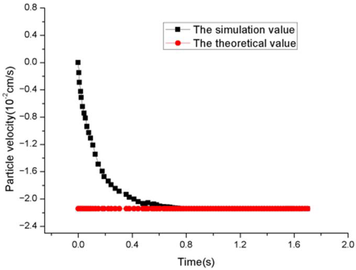
3.1. Settlement of Small, Spherical 3D Particles in Infinite Length Pipeline

Glowiski [24] proposed that when the physical parameters of a ball are fixed, the final stable settlement velocity of the ball in the infinite pipe is also fixed. When the fluid is at a low Reynolds number, the influence of viscous force on the flow field is greater than that of inertial force and the disturbance of the flow velocity in the flow field will be attenuated due to the viscous force, meaning the fluid flow will be relatively stable.

The final settling velocity of spherical particles can be calculated by [15]:

$$v=\frac{D^2({\rho }_S-{\rho }_l)\mathbf{g}}{16K\eta }$$

(27)

where D is the diameter of the spherical particle, ${\rho }_s$ and ${\rho }_l$ are the densities of the spherical particles and fluid, respectively, g is the acceleration of gravity, and $\eta$ is the dynamic viscosity of the fluid. Here, $K$ is the correction factor of the resistance of the pipe wall to the particle, representing the influence of the long pipe wall on the particle:

$$K=\frac{1}{\ln W_f-0.9157+1.7244{(W_f)}^{-2}-1.7302{(W_f)}^{-4}+2.4056{(W_f)}^{-6}-4.5913{(W_f)}^{-8}}$$

(28)

In the simulation, the calculation domain is divided into 80 × 80 × 500 cubic grids, the grid size h is 0.003 cm, the diameter of the 3D spherical particle is 0.048 cm, and the width between plates L is 0.24 cm. The density of the fluid is ${\rho }_l$ = 1.0 g/cm³ , the density of solid particle is ${\rho }_s$ = 1.02 g/cm³, the acceleration of gravity is $g$ = 980.0 cm/s², and the viscosity of the fluid is $\eta$ = 0.33 g/(cm∙s). At the initial time, the static spherical particle is placed at the location indicated in Figure 1. The velocity at the entrance boundary is 0, and the velocity derivative at the exit boundary is 0. The non-equilibrium extrapolation scheme is used to deal with six wall boundaries.

When the calculation time $\Delta t$ = 3.125 × 10⁻⁵ s, the maximum Reynolds number is 469.37, which is in good agreement with the results from the studies by Wan [25], Uhlmann [26], and Glowiski [24]. In this paper, the spherical particle is always located on the central axis of the pipe. The spatial discretization scheme is highly symmetrical, and the numerical disturbance caused by the wall resistance is small.

Figure 2 demonstrates that the spherical particle falls from the static state, then, because the gravity is greater than the resultant force of buoyancy and resistance, the particle continues to accelerate, while the resistance also increases and the acceleration decreases. Finally, the three forces of gravity, buoyancy, and resistance are balanced. The velocity is consistent with the theoretical value when it is stable, demonstrating that the treatment of the moving boundary of the solid–liquid interface is reasonable.

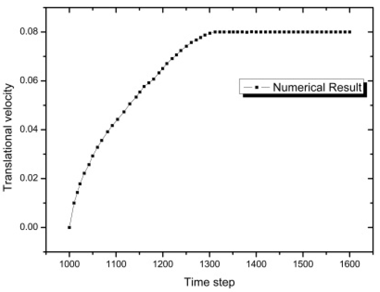
3.2. Verification of the Translation of a Single Dendrite

The computational domain is divided into 110 × 110 × 110 cubic grids with a size of 1 μm. The initial composition of the liquid phase $C_0=4.7\%$. The left boundary of the simulation domain is a constant entrance velocity ${\mathit{u}}_0=0.08 \mathrm{cm}/\mathrm{s}$, the right boundary is a fully developed boundary, and the other four boundaries are sliding boundaries. At the initial time, a nucleus is placed at (50, 20, 50), the $f_s$ of this seed is 0.2, and the preferential growth angle is 0 rad. At the beginning, the effect of the flow field on dendrite growth is ignored, so that the dendrite grows in a static state. When the number of time steps is 1000, the growth of the dendrite is ignored, and a uniform flow field is added into the domain. The dendrite begins to move horizontally due to the flow field.

Dendrites accelerate along the horizontal direction with the pipeline flow, and the resistance of the dendrites increases as the velocity of the dendrites increases. When the drag is equal to the traction force, the dendrite will move at a uniform velocity in the horizontal direction. In order to quantitatively describe the velocity of the dendrite, the movement velocity–time curve of dendrite is provided in Figure 3, which demonstrates that when the dendrite reaches a stable state, the velocity is the same as that of the fluid.

The change degree of the dendrite morphology is quantitatively described by introducing $\lambda$:

$$\lambda =(f_s^1-f_s^0)/f_s^0$$

(29)

Here, $f_s^0$ is the solid fraction before the dendrite movement and $f_s^1$ is the solid fraction after the dendrite movement; $\lambda$ is approximately 0 at any time, which quantitatively demonstrates that the solid fraction will not be lost due to the translation.

4. Results and Discussions

The calculations in this paper are based on the following assumptions: (1) The melt is considered as an incompressible Newtonian fluid. (2) The temperature of the six walls in the computational domain is 913 K and the initial undercooling is 4 K. (3) The thermal conductivity of the solid phase and liquid phase is the same and the heat transfer boundary condition is adiabatic. (4) Solute diffusion only occurs in the liquid phase; there is no solute diffusion in the solid phase. The solid phase is homogeneous, and the mass transfer boundary condition is a non-diffusion boundary condition. (5) The impacts of dendrite collisions are ignored.

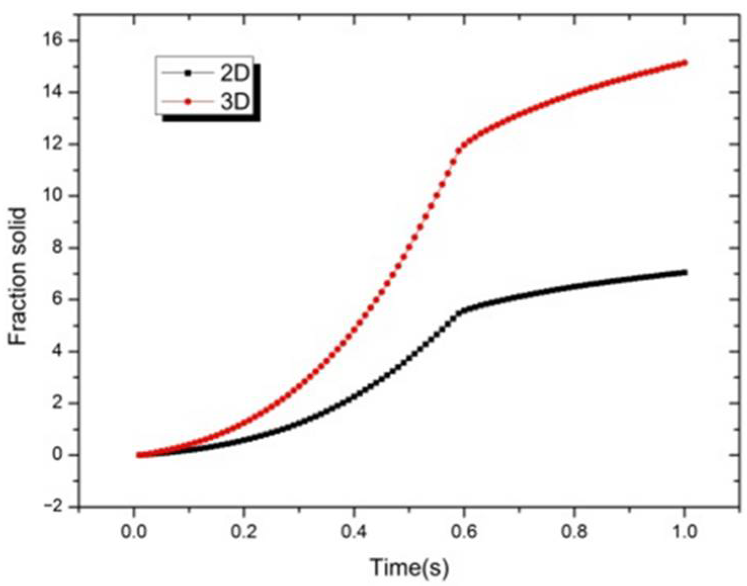
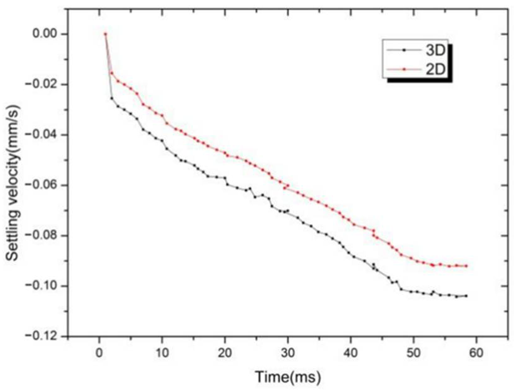
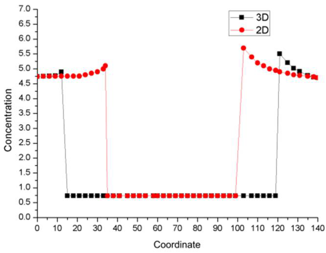
4.1. Comparison of Simulation Results for 3D and 2D Models under Moving Conditions

In 3D calculationg, the computational domain is divided into 140 × 140 × 140 cubic grids with a size of 0.5 μm. At the beginning of the solidification, a seed with an initial preferential growth angle of 0 rad is placed at the upper position (70, 70, 100) of the calculation domain and the nucleus grows along the coordinate axis. The initial composition of the liquid phase is $C_0$ = 4.7%, while $k$ is the equilibrium distribution coefficient; therefore, the solid solute composition of the nucleus is $k{C}_0$ and the Prandtl number is 0.7. The density of the solid phase of the Al-4.7% Cu alloy is higher than that of the liquid phase, and the primary dendrites formed by solidification will grow while settling in the melt, consistent with the experimental observations [27,28]. The 2D simulation calculation domain is 400 × 800 and other parameters are consistent with those in the 3D model.

Generally speaking, the solute distribution around the static dendrite is relatively uniform, meaning the growth velocity of the dendrite trunks should be the same and should exhibit symmetrical growth in the six directions. Figure 4a demonstrates the streamline distribution as the 3D dendrite is falling; in the figure, the flow direction of the solution around the dendrite is upward. As the dendrite moves downward, the melt will wash the latent heat and solute released by the dendrite arm from the downstream tip to the upstream tip, meaning the growth of the dendrite is asymmetric.

In addition, as the dendrite falls, more solute is discharged from the upper tip of the dendrite and the diffusion speed of the discharged solute is not as fast as the accumulation speed of the solute, meaning there will be a high-concentration zone of solute enrichment in the upper part. The secondary dendrites also hinder the diffusion of the solute, resulting in the inhibition of the growth of the upper dendrite arm. This is consistent with the phenomenon observed by Badillo et al. [29].

As demonstrated in Figure 4a, in the 3D simulation process, the 3D streamline forms a circulation motion along the primary dendrite trunk in the vertical direction. In the horizontal direction, the streamline passes through the secondary dendrite arm, demonstrating the spatial fluid flow more realistically. In the 2D simulation process (as demonstrated in Figure 4b), a clockwise circulation motion is formed on the left side of the dendrite and a counterclockwise circulation motion symmetrical to the left side is formed on the right side of the dendrite. It can be observed that the solution is hindered when it flows to the dendrite trunk and can only bypass the dendrite tip along the dendrite arm, which makes it difficult for the solute to drain away, creating a high-concentration zone. Through this comparison, it is obvious that the calculation of dendrite movement and growth and solute transport under 3D conditions is more realistic.

Figure 5 demonstrates the curves for the total solid fraction over time under 3D and 2D conditions, which represent the growth velocity of the dendrite. It can be observed that the growth velocity of the 3D equiaxed crystal is faster, which is about 2.7 times that of the 2D equiaxed crystal under the same conditions; this is mainly because the 3D model has more diffusion directions (along the Z axis) than the 2D model. Therefore, the solute discharged from the tip is more easily diffused, which makes the concentration gradient of the solute at the tip front larger than that of the 2D model. This is consistent with the conclusions drawn by Eshraghim et al. [30].

Figure 6 demonstrates a comparison of the falling velocity rates for 2D and 3D dendrites. It can be observed from the figure that the 3D dendrite and the 2D dendrite start to fall at the same time, but the falling velocity for the 3D dendrite is obviously higher than that of the 2D dendrite at the same time point. The main reason for this phenomenon is that the solute discharged from the 3D dendrite tip diffuses faster and more Cu is discharged from the dendrite tip. The density of Cu is higher than for Al, resulting in a downward flow field around the dendrite tip. The downward flow field around the 3D dendrite is stronger, causing the dendrite to fall faster.

Figure 7 demonstrates the concentration distribution along the dendrite axis in 2D and 3D. In the figure, the ordinate represents the solute content, and the abscissa represents the grid number of the dendrite cross-section. The left side of the line represents the concentration distribution in front of the upstream tip and the right side represents the concentration distribution in the downstream tip. It can be observed from the figure that the 2D and 3D concentration distributions display a certain consistency. The lowest horizontal line in the figure represents the solute content in the solid phase inside the equiaxed crystal, with a low concentration of about 0.78%. The solute concentration increases sharply at the solid–liquid interface and the highest solute content reaches 5.9%. Then, the concentration in the liquid phase decreases with the distance from the dendrite. On the whole, the concentration at the front of the upstream tip is significantly lower than that at the downstream tip and the concentration gradient at the front of the upstream tip is greater than that at the downstream tip. It can be observed that the solute concentration at the front of the 3D dendritic tip is lower than that at the 2D dendritic tip, and the solute diffusion layer at the 3D dendritic tip is thinner than that at the 2D dendritic tip. This is because, in the process of 3D dendrite movement, the melt drives the solute at the upstream tip to flow to the downstream tip, and also accelerates the temperature diffusion, shortens the solute diffusion layer thickness at the interface front of upstream tip, and increases that at the front of downstream tip.

The 3D dendrite arm is longer, which can affect the flow field in a larger range when it moves, meaning the solute discharged from the tip has a larger diffusion range. The 3D fluid can flow around the dendrite arm and wash the solute away directly from the side of the dendrite arm, which greatly shortens the diffusion distance and reduces the concentration enrichment.

In summary, there are many differences between the 2D model and the 3D model in the calculation of the motion of equiaxed crystals. Obviously, the 3D CA–LBM model can more accurately describe the movement and growth of equiaxed crystals.

4.2. Study of the Movement Behavior of Multiple Dendrites

The calculation parameters in this section are consistent with those in Section 4.1. Figure 8 demonstrates the dendrite morphology and partial streamline distribution of the five dendrites in the stationary state and the moving state. It can be observed from the streamline distribution in Figure 8 that as the dendrite falls, due to the flow of the melt, a cluster of closed streamlines around the dendrite is formed. The streamline directions of the 3D vortex are upward near the equiaxed crystal and downward far away from the equiaxed crystal, which means that the flow field always flows around the dendrite. In the moving state, the streamlines are distributed among the dendrites, which indicates that the interactions among the dendrites cause the solution convection. The independent fluid vortices begin to contact and gradually merge, the flow field in the same direction is superimposed and enhanced, and the flow field in the opposite direction is partially offset. When multiple equiaxed crystals are falling, because there is no external forced convection in this paper, the flow field produced by the natural convection driving the movement of dendrites is weak and multiple dendrites hinder each other, so the falling distance is small.

Figure 9 demonstrates the relationship between the movement velocity and time, which can quantitatively describe the movement process for the dendrites. The results indicate that all of the dendrites fall at first, then the acceleration decreases, and then the velocity decreases, whereby their falling velocity is less than that of a single dendrite. For dendrite 2, because it is far away from other dendrites, the interaction between dendrite 2 and other dendrites will be smaller, and the solute buoyancy and thermal buoyancy caused by the solute and heat discharged from its tip will have a greater impact on the falling velocity. For dendrite 5, it is close to dendrite 3. When dendrite 3 falls, the solute discharged from its tip will hinder the falling of dendrite 5 and the thermal buoyancy will cause an upward flow field around dendrite 5, which will slow down the falling velocity. For dendrite 3, because it is in the middle of these dendrites, it will be affected by the upward combined flow field of dendrites 1 and 2 and the downward flow field of dendrites 4 and 5; therefore, the dendrites will be affected by the 3D vortex generated by the movement of other dendrites in the process of falling, so the falling velocity curve presents a fluctuating trend.

The 3D vortex around a dendrite hinders its vertical drop, and because the streamline around the dendrite not only flows vertically down along the Z axis but also flows around the dendrite, the surrounding solution will produce lateral force on the dendrite in the horizontal plane and the dendrite will also move in the horizontal direction.

The lateral displacement of the dendrites is presented in

Table 2. X-direction coordinate changes for the dendrites.

Time(s)	No. 1	No. 2	No. 3	No. 4	No. 5
0.1	+1	0	+1	+1	−1
0.2	+1	0	0	−2	+1
0.3	+2	+1	+2	0	0
0.4	0	+1	+1	+1	+1

and

Table 3. Y-direction coordinate changes for the dendrites.

Time(s)	No. 1	No. 2	No. 3	No. 4	No. 5
0.1	+2	−2	+1	−5	0
0.2	+1	−1	+3	−2	0
0.3	0	−2	+1	0	0
0.4	+1	0	+1	−1	+1

.

Here, − means that the dendrite moves to the negative direction of the coordinate axis and + means that the dendrite moves to the positive direction of the coordinate axis. The displacement distance is calculated by the position of the center of mass. According to the displacement of dendrites, it can be observed that the lateral forces acting on the dendrites at different positions are not the same. Under the action of the flow field generated by other dendrites, dendrite 1 will move to the positive directions of the x-axis and y-axis, while dendrite 2 will move to the positive direction of the x-axis and negative direction of the y-axis. Compared with dendrite 1, dendrite 2 is in a more central position and is closer to other dendrites, so it has a stronger effect and longer horizontal displacement distance. Other dendrites are similarly affected, so will not be discussed here.

5. Conclusions

In this paper, the LBM–CA model, Ladd method, non-equilibrium extrapolation method, and Newton’s law of classical mechanics were combined to establish a 3D model for calculating the motion and growth process of equiaxed crystals for the first time. The model was verified and the motion of single and multiple 3D equiaxed crystals was calculated. Compared with the 2D method, the difference between the two growth models was analyzed. The results demonstrated that: (1) In the 3D simulation, the 3D eddy current drove the solute to diffuse around the dendrite, so the solute diffusion was faster, the solute concentration between dendrites was lower, and the falling and growth speeds were faster than in the 2D model. Therefore, the 3D model more truly reflected the movement of equiaxed crystals and the melt flow around dendrites. (2) The growth modes of dendrites in motion are different from that in static state, and multiple dendrites will influence each other in the processes of movement and growth, changing the original movement and growth modes.

References

1. Appolaire, B.; Albert, V.; Combeau, H.; Lesoult, G. Free growth of equiaxed crystals settling in undercooled NH4Cl–H2O melts. Acta Mater. 1998, 46, 5851–5862. [Google Scholar] [CrossRef]
2. Do-Quang, M.; Amberg, G. Simulation of free dendritic crystal growth in a gravity environment. J. Comput. Phys. 2008, 227, 1772–1789. [Google Scholar] [CrossRef]
3. Badillo, A.; Ceynar, D.; Beckermann, C. Growth of equiaxed dendritic crystals settling in an undercooled melt, Part 2: Internal solid fraction. J. Cryst. Growth. 2007, 309, 216–224. [Google Scholar] [CrossRef]
4. Wu, M.; Ludwig, A. Modeling equiaxed solidification with melt convection and grain sedimentation—I: Model description. Acta Mater. 2009, 57, 5621–5631. [Google Scholar] [CrossRef]
5. Karagadde, S.; Bhattacharya, A.; Tomar, G.; Dutta, P. A coupled VOF-IBM-enthalpy approach for modeling motion and growth of equiaxed dendrites in a solidifying melt. J. Comput. Phys. 2012, 231, 3987–4000. [Google Scholar] [CrossRef]
6. Medvedev, D.; Varnik, F.; Steinbach, I. Simulating Mobile Dendrites in a Flow. Procedia Comput. Sci. 2013, 18, 2512–2520. [Google Scholar] [CrossRef]
7. Kharicha, A.; Stefan-Kharicha, M.; Ludwig, A.; Wu, M. Simultaneous observation of melt flow and motion of equiaxed crystals during solidification using a dual phase Particle Image Velocimetry technique. Metall. Mater. Trans. A 2012, 44, 650–660. [Google Scholar] [CrossRef]
8. Rojas, R.; Takaki, T.; Ohno, M. A phase-field-lattice Boltzmann method for modeling motion and growth of a dendrite for binary alloy solidification in the presence of melt convection. J. Comput. Phys. 2015, 298, 29–40. [Google Scholar] [CrossRef]
9. Takaki, T.; Rojas, R.; Ohno, M.; Shimokawabe, T. GPU phase-field lattice Boltzmann simulations of growth and motion of a binary alloy dendrite. IOP Conf. Ser. Mater. Sci. Eng. 2015, 84, 012066. [Google Scholar] [CrossRef] [Green Version]
10. Ludwig, A.; Vakhrushev, A.; Wu, M.; Holzmann, T.; Kharicha, A. Simulation of Crystal Sedimentation and Viscoplastic Behavior of Sedimented Equiaxed Mushy Zones. Trans. Indian Inst. Met. 2015, 68, 1087–1094. [Google Scholar] [CrossRef]
11. Xin, B.; Yun, C.; Xiu, H.; Dian, Z.; Tong, Z. Modeling of coupled motion and growth interaction of equiaxed dendritic crystals in a binary alloy during solidification. Sci. Rep. 2017, 7, 45770. [Google Scholar]
12. Takaki, T.; Sato, R.; Rojas, R.; Ohno, M.; Shibuta, Y. Phase-field lattice Boltzmann simulations of multiple dendrite growth with motion, collision, and coalescence and subsequent grain growth. Comp. Mater. Sci. 2018, 147, 124–131. [Google Scholar] [CrossRef]
13. Conti, M. Solidification of binary alloys: Thermal effects studied with the phase-field model. Phys. Rev. E 1997, 55, 765–771. [Google Scholar] [CrossRef]
14. Jelinek, B.; Eshraghi, M.; Felicelli, S.D.; Peters, J. Large-scale parallel lattice Boltzmann-cellular automaton model of two-dimensional dendritic growth. Comput. Phys. Commun. 2014, 185, 939–947. [Google Scholar] [CrossRef]
15. Liu, L.; Pian, S.; Zhang, Z.; Bao, Y.; Li, R.; Chen, H. A cellular automaton-lattice Boltzmann method for modeling growth and settlement of the dendrites for Al-4.7%Cu solidification. Comp. Mater. Sci. 2018, 146, 9–17. [Google Scholar] [CrossRef]
16. Bai, Y.; Wang, Y.; Zhang, S.; Wang, Q.; Li, R. Numerical model study of multiple dendrite motion behavior in melt based on LBM–CA method. Crystals 2020, 10, 70. [Google Scholar] [CrossRef] [Green Version]
17. Ladd, A.J. Numerical simulations of particulate suspensions via a discretized Boltzmann equation Part 1. Theoretical foundation. J. Fluid Mech. 1994, 271, 285–310. [Google Scholar] [CrossRef] [Green Version]
18. Sun, D.; Zhu, M.; Pan, S.; Yang, C. Lattice Boltzmann modeling of dendritic growth in forced and natural convection. Comput. Math. Appl. 2011, 61, 3585–3592. [Google Scholar] [CrossRef] [Green Version]
19. Li, R.; Shen, H.; Feng, C.; Pan, H.; Feng, C. A new solute partitioning model for cellular automata simulation of microstructure and its computational verification. Acta Phys. Sin. 2013, 62, 475–480. (In Chinese) [Google Scholar]
20. Pan, S.; Zhu, M. A three-dimensional sharp interface model for the quantitative simulation of solutal dendritic growth. Acta Mater. 2010, 58, 340–352. [Google Scholar] [CrossRef]
21. Yin, H.; Felicelli, S.D.; Wang, L. Simulation of a dendritic microstructure with the lattice Boltzmann and cellular automaton methods. Acta Mater. 2011, 59, 3124–3136. [Google Scholar] [CrossRef]
22. Mohsen, A.Z.; Hebi, Y. Comparison of cellular automaton and phase field models to simulate dendrite growth in hexagonal crystals. J. Mater. Sci. Technol. 2012, 28, 137–146. [Google Scholar]
23. Pian, S.; Zhang, Z.; Bao, Y.; Liu, L.; Li, R. Simulation of dendrite morphology and composition distribution of Al-4.7%Cu alloy based on three dimensional LBM–CA model. Mater. Rev. 2017, 20, 143–149. (In Chinese) [Google Scholar]
24. Glowinski, R.; Pan, T.W.; Hesla, T.I.; Joseph, D.D.; Periaux, J. A Fictitious Domain Approach to the Direct Numerical Simulation of Incompressible Viscous Flow past Moving Rigid Bodies: Application to Particulate Flow. J. Comput. Phys. 2001, 169, 363–426. [Google Scholar] [CrossRef] [Green Version]
25. Wan, D.; Turek, S. An efficient multigrid-fem method for the simulation of solid–liquid two phase flows. J. Comput. Appl. Math. 2007, 203, 561–580. [Google Scholar] [CrossRef] [Green Version]
26. Uhlmann, M. Numerical simulation of particulate flows: Comparison of fictitious domain methods with direct and indirect forcing. In Proceedings of the 10th European Turbulence Conference, Advances in Turbulence X, Trondheim, Norway, 29 June 2004–2 July 2004; pp. 415–418. [Google Scholar]
27. Wang, C.Y.; Beckermann, C. Equiaxed dendritic solidification with convection: Part II. Numerical simulations for an Al-4wt pct Cu alloy. Metall. Mater. Trans. A 1996, 27, 2765–2783. [Google Scholar] [CrossRef]
28. Chen, Y.; Li, D.Z.; Billia, B.; Nguyen-Thi, H.; Qi, X.B.; Xiao, N.M. Quantitative phase-feld simulation of dendritic equiaxed growth and comparison with in situ observation on Al-4wt.%Cu alloy by means of synchrotron X-ray radiography. ISIJ Int. 2014, 54, 445–451. [Google Scholar] [CrossRef] [Green Version]
29. Badillo, A.; Ceynar, D.; Beckermann, C. Growth of equiaxed dendritic crystals settling in an undercooled melt, Part 1: Tip kinetics. J. Cryst. Growth 2007, 309, 197–215. [Google Scholar] [CrossRef]
30. Eshraghi, M.; Hashemi, M.; Jelinek, B.; Feliceli, S.D. Three-Dimensional Lattice Boltzmann Modeling of Dendritic Solidification under Forced and Natural Convection. Metals 2017, 7, 474. [Google Scholar] [CrossRef] [Green Version]
Figure 1. Diagram of a ball falling: (a) 3D diagram; (b) plane diagram.
Crystals 11 01056 g001
Figure 2. Settling velocity for the spherical particle.
Crystals 11 01056 g002
Figure 3. Translational velocity curve for the dendrite in the pipe flow.
Crystals 11 01056 g003
Figure 4. The streamline distribution of 3D and 2D: (a) flow field as the 3D dendrite falls, and (b) flow field as the 2D dendrite falls.
Crystals 11 01056 g004
Figure 5. Curves of the total solid fraction over time under 3D and 2D conditions.
Crystals 11 01056 g005
Figure 6. Falling velocity rates for 2D and 3D dendrites.
Crystals 11 01056 g006
Figure 7. Concentration distribution on the center line of the section.
Crystals 11 01056 g007
Figure 8. Morphology and streamline distribution for multiple 3D dendrites: (a) static state, and (b) moving state.
Crystals 11 01056 g008
Figure 9. Falling velocity rates for dendrites 2, 3, and 5.
Crystals 11 01056 g009