Article

Estimation of Ferroelectric Material Properties and Phase-Shifter Design Key Parameters Influence on Its Figure of Merit for Optimization of Development Process

Faculty of Electronics, Saint Petersburg Electrotechnical University “LETI”, Prof. Popova Str. 5, Saint Petersburg 197376, Russia
*
Author to whom correspondence should be addressed.
Crystals 2021, 11(5), 538; https://doi.org/10.3390/cryst11050538
Submission received: 30 March 2021 / Revised: 27 April 2021 / Accepted: 4 May 2021 / Published: 12 May 2021
(This article belongs to the Special Issue Ferroelectrics Materials for Microwave Devices)

Abstract

:
A model of the estimation of the ferroelectric-based phase-shifter figure of merit concerning the material properties and phase-shifter design parameters is presented. The influence of ferroelectric material tunability and losses on phase-shifter characteristics are analyzed. Two approaches to phase-shifter design (transmission line and band-pass filter) are considered. The review of the published results on the ferroelectric phase-shifter design was performed to approve the method proposed. Recommendations to optimize the phase-shifter development process are suggested on the basis of the elaborated model and analysis performed.

1. Introduction

Phase-shifter can be considered a key element of modern microwave electronics. Excluding digital phase shifters, switching a different number of transmission line sections, there are several methods to design the phase-shifters with an analog control: tunable transmission lines (regular or periodically loaded), tunable wideband band-pass filters and reflection-type phase-shifters. The first two methods are considered in the present work.
The main characteristic of the yield of a phase-shifter is a figure of merit (FoM) defined as
FoM = Δ ϕ L ,
where Δ ϕ is the phase-shift (actually the difference between phase-shifts for two states—zero bias voltage and maximum bias voltage for voltage-controlled devices) and L is the insertion loss of a phase-shifter.
Application of ferroelectric (FE) films for the microwave devices requires a preliminary estimation of the device’s parameters, relying on the electrophysical characteristics of the FE tunable element (capacitor) or the FE film itself, to choose the optimal design option. Commonly, the estimation of FE films’ applicability from the point of their microwave properties is carried out based on the FE capacitor figure of merit (commutation quality factor (CQF)) proposed by Vendik [1,2,3,4,5]
CQF = ( K 1 ) 2 K tan δ 1 tan δ 2 ,
where K = C 1 / C 2 is tunability of the capacitance C under the bias voltage U b from the initial capacitance C 1 = C ( 0 ) to the capacitance under bias C 2 = C ( U b ) and tan δ 1 and tan δ 2 are values of the loss tangent of the capacitor with and without bias, respectively. The CQF parameter allows choosing the best one from a number of tunable capacitors with various combinations of tunability and dielectric losses.
The development task requires taking into account the features of the design, particularly losses in the other parts of the device except for the FE tunable element. The estimations of the figure of merit have been developed for the phase-shifters based on the regular transmission line [1,2,3,6] and on the periodically loaded transmission line [7] and for reflection type phase-shifters [5,8]. The figure of merit has also been introduced for the ferroelectric based band-pass filters (BPF) [9,10]. However, the figure of merit for the phase-shifter based on the microwave band-pass filter (BPF) has not yet been considered.
There is another concern in the ferroelectrics application at microwaves. The microwave losses of the FE tunable capacitor depend on a control voltage, which leads to a variation of the microwave device’s insertion loss. Thus, undesired amplitude modulation emerges. This effect can be compensated by changing the inclusion of the tunable element into the device. Such compensation has been considered for the periodically loaded transmission line [7]. However, the application of the ferroelectrics in a condition of the variated inclusion requires the special estimation of the ferroelectrics figure of merit.
In the present work, an approach to estimate the figure of merit of a microwave phase-shifter based on the band-pass filter structure compared with the one based on a tunable transmission line is considered in detail. The above definition of the CQF parameter is expanded, considering the possibility of the FE capacitor inclusion variation into a microwave device.

2. Methods

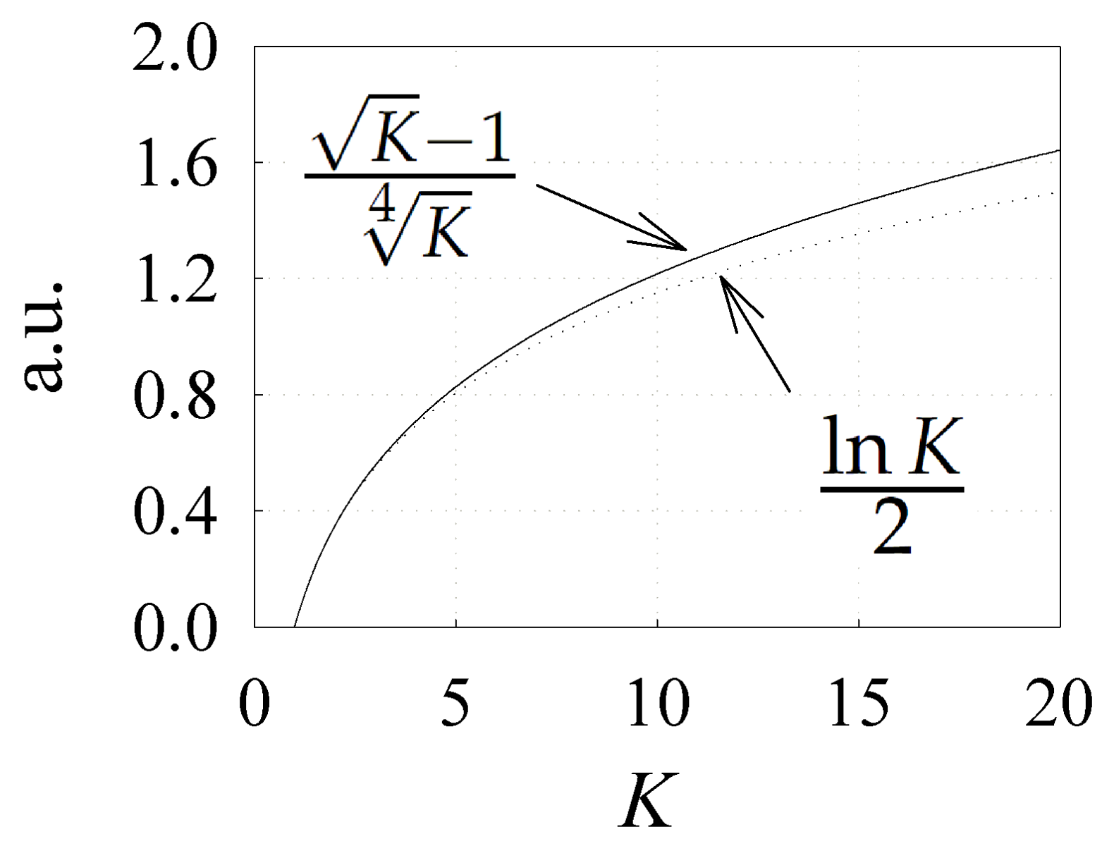
2.1. Figure of Merit of the Transmission Line Based Phase-Shifter

The figure of merit for the phase-shifters based on the transmission line is considered in previous publications for the cases of lossless conductors [1,3] (superconductor phase-shifter) and lossy conductors [6]. However, we deliberately derive all expressions again to keep the continuity of the presentation.
Phase-shifter can be designed based on the transmission line section, where the propagation constant β can be changed (for example, by the tuning of a ferroelectric by a bias voltage). The phase in transmission line is defined as ϕ = β l , β = 2 π / Λ , Λ = λ ε , where l is the length of the section, Λ is the wavelength in the transmission line, λ is the wavelength in a free space and ε is the effective permittivity of the transmission line so that ε = λ / Λ .
Phase in the transmission line can be changed by the tuning the ε so that phase-shift Δ ϕ is
Δ ϕ = 2 π l 1 λ 0 ε 1 ε 2 ,
where λ 0 is the operating wavelength of the phase-shifter and ε 1 = ε ( 0 ) and ε 2 = ε ( U b ) are the permittivity at zero voltage and under bias, respectively.
Insertion loss per unit of the transmission line length α can be defined as [11]
α = 8.68 π ε Q λ ,
where Q is transmission line Q-factor. The mean insertion loss value of the line being tuned is
α mean = 8.68 π ε 1 ε 2 4 Q 1 Q 2 λ .
The mean Q-factor, in turn, is
Q mean = Q 1 Q 2 = Q 0 1 + tan δ 1 tan δ 2 Q 0 ,
where tan δ 1 and tan δ 2 are dielectric loss tangent values at zero voltage and bias voltage, respectively, and Q 0 is the inherent Q-factor of transmission line determined by the conductive loss (see Appendix A).
The length of the line required to shift the phase by 2 π is defined from Equation (3), substituting Δ ϕ = 2 π :
l line = λ ε 1 ε 2 .
Then, the mean insertion loss for the tunable transmission line with the length l l i n e that shifts the phase by 2 π can be written from Equations (5)–(7) as
L mean = α mean l line = 8.68 π 1 Q 0 ε 1 ε 2 4 ε 1 ε 2 + 8.68 π ε 1 ε 2 4 tan δ 1 tan δ 2 ε 1 ε 2 .
Equation (8) can be transformed, taking into account the tunability, to K ε = ε 1 / ε 2 , as
L mean = 8.68 π 1 Q 0 K ε 4 K ε 1 + 8.68 π K ε 4 tan δ 1 tan δ 2 K ε 1 .
The tunability K ε can also be expressed as K = C 1 / C 2 as in Equation (2), but, in this case, C 1 and C 2 are the capacitances of the transmission line at zero voltage and at bias voltage, respectively.
From Equation (9), the figure of merit of the transmission line can be defined as
q line = K 1 K 4 tan δ 1 tan δ 2 ,
and the insertion loss in the phase-shifter based on the tunable transmission line can be written as
L = 8.68 π 1 Q 0 K 4 K 1 + 8.68 π 1 q line .
The figure of merit q line defined by Equation (10) compares with the CQF defined by Equation (2) as
q line 2 = CQF .
The insertion loss defined by Equation (11) is transformed to figure of merit of phase-shifter as
FoM = 360 deg / L .
It can be shown that the insertion loss L transformed to FoM by Equation (13) corresponds to the expressions published earlier (see [1,3] at Q 0 = , lossless conductors, and [6]).
Note that Equation (11) is valid for the regular tunable lines as well as for the periodically loaded tunable lines.

2.2. Figure of Merit of the Tunable Element Included in the Microwave Resonator

The efficiency of tuning the resonant frequency of a resonator by tuning the capacitance of a capacitor included in it depends on both the capacitance of the capacitor and the characteristics of the resonator. To define this efficiency, a parameter was introduced by Kozyrev et al. [12]: the inclusion coefficient. Unfortunately, there is no detailed derivation of the expressions associated with this parameter in the reviewed publications. Therefore, we define the inclusion coefficient and its relationship with the Q-factor of the resonator in Appendix A, and the derivation of formulas for calculating the inclusion coefficient is presented in Appendix B.
For a the tunable resonator with a capacitor, as a tuning element, one can write (see Equation (A29) in Appendix B).
d f f = ξ 2 d C C ,
where ξ is the inclusion coefficient.
The value of ξ depends both on the size and design of a particular resonator and on the value of the capacitance C. In Figure 1 (see Appendix B), ξ is plotted versus capacitance for f 0 = ω 0 / 2 π = 1 GHz and Z 0 = 50 Ohm and examples of the various behavior of ξ ( C ) are shown. Curves refer to the resonator with short-circuit (SC) and open-circuit (OE) conditions at the termination, and n is an integer referring to the resonance order.
Different sections of the ξ ( C ) curves can be approximated as
ξ = ξ 0 C m ,
where ξ 0 is the constant with the dimension of C ( m ) and m is an integer. The sections near the maximum of the curves can be approximated with m = 0 and the other sections with m 0 .
The frequency tuning can be found by integrating Equation (14) from C 1 = C ( 0 ) to C 2 = C ( U b ) and from initial resonance frequency f 1 to the frequency under bias f 2 , substituting ξ with the the specific dependence (Equation (15)). For the region of the constant inclusion coefficient m = 0 , one can integrate
C 1 C 2 ξ 0 2 d C C = f 1 f 2 d f f ,
C 1 C 2 ξ 0 2 d C C = ξ 0 2 ln ( C 2 ) ln ( C 1 ) = ξ 0 2 ln C 1 C 2 = ξ 0 2 ln K ,
f 1 f 2 d f f = ln f 2 f 1 = ln f 1 + Δ F t f 1 Δ F t f ,
where Δ F t is the frequency tuning of the resonator, Δ F t = f 2 f 1 f 1 , f is the resonance frequency, K = C 1 / C 2 is the tunability of the capacitor and C 1 > C 2 , f 1 < f 2 . From Equations (17) and (18), one can write that
ξ 0 = 2 Δ F t f 1 ln K .
The unloaded Q-factor of a microwave resonator with a real tuning element ( tan δ 0 ) can be expressed as (Appendix A)
Q = Q 0 1 + ξ Q 0 tan δ .
where tan δ is the loss tangent of the capacitor and Q 0 is the inherent quality factor of the resonator with a lossless capacitor. One can see that the modulation of tan δ under the tuning can be compensated by choosing the proper section of the ξ ( C ) dependence (Figure 1).
Substituting Equation (19) into Equation (20), one can calculate the Q-factor of the resonator for the initial and final capacitances C 1 and C 2 :
Q 1 , 2 = Q 0 1 + 2 Δ F t f 1 ln K Q 0 tan δ 1 , 2 .
If the inherent Q-factor of the resonator is very high so that ξ Q 0 tan δ 1 , then
Q 1 , 2 1 2 Δ F t f ln K tan δ 1 , 2 ,
and the mean Q-factor of the resonator can be defined as
Q m e a n = Q 1 Q 2 = 1 2 Δ F t f ln K tan δ 1 tan δ 2 .
Let us define the figure of merit for the tunable capacitor as
q = ln K 2 tan δ 1 tan δ 2 .
Since Q m e a n = f / Δ f m e a n , where Δ f m e a n is the mean bandwidth of the resonator, the figure of merit q value is the resonator frequency tuning in units of the bandwidths q = Δ F t / Δ f m e a n .
In the general case ξ Q 0 tan δ 1 of Equation (23),
Q m e a n = Q 0 1 + 2 Δ F t f Q 0 q .
For the regions with varying inclusion coefficient (Figure 1), where it is defined by Equation (15) with m 0 , one can write
Δ F t f = C 1 C 2 ξ 0 C m 2 d C C = ξ 0 2 C 1 C 2 C m 1 d C = ξ 0 2 C 1 m C 2 m m ,
ξ 0 = 2 Δ F t f m C 1 m C 2 m .
Substituting Equation (27) into Equation (20), the figure of merit of the capacitor for m 0 is
q = 1 2 m K m 1 K m / 2 1 tan δ 1 tan δ 2 .
A limit of Equation (28) at m 0 leads to Equation (24).

2.3. Parameters of the Microwave Bandpass Filter Based on FE Tunable Element

Several tunable microwave resonators can be arranged in a bandpass filter (BPF). Estimation of the efficiency of such structure is a complicated task because the magnitude and phase characteristics of the filters are described by the complicated semi-empirical expressions and tables [13]. The approach to obtain the closed-form expressions for calculating the figure of merit of the phase-shifter based on BPF tuned by the FE tunable is presented below.
To analyze the BPF parameters, the Q-factor of the resonator (see Equations (19) and (20)) is useful to write as
1 Q = 1 Q 0 + 1 q Δ F t f
The insertion loss in the bandwidth of the BPF L BPF is defined as [13]
L BPF 8.68 C n Q ω ,
where C n is the coefficient defined by the number of resonators n, Q is the Q-factor of each resonator composing the BPF, ω = Δ f f / f is the relative bandwidth, Δ f f is the absolute bandwidth of BPF and f is the central frequency of the filter that is equal to the resonance frequency of the resonator.
Substituting Equation (29) into Equation (30), one can write
L BPF = 8.68 C n 1 Q ω + 8.68 C n 1 q Δ F t Δ f f .
A similar equation was obtained by Kozyrev et al. [9].

2.4. Figure of Merit of the Band-Pass Filter Based Phase-Shifter

The basic operating principles of a BPF-based phase-shifter can be explained with reference to Figure 2. In the figure, the frequency response L (solid lines, where blue is for U = 0 and red is for U = U b ) and the phase response ϕ (dashed lines) are presented. When the filter is tuned (central frequency f 0 is shifted by Δ F t ), both L and ϕ are shifted, thus the phase-shift Δ ϕ (difference of the phase response) is achieved in the bandwidth of the phase-shifter Δ f PS = Δ f f Δ F t (marked by wide green line).
Since Chebyshev filters are the most effective as a phase-shifter, this type of filter was used to analyze the frequency response and phase response. The approximation of the phase-shifter figure of merit requires determining the phase shift and insertion loss in the bandwidth. However, these parameters, in turn, depend on the filter center frequency shift, the number of resonators and their Q-factors. The phase shift’s dependencies on the number of resonator n at the Δ F t / Δ f f for different values of the ripple Δ A are presented in [13]. In Figure 3, the dependencies are shown for Δ A = 0.011 dB (for other values of Δ A , the dependencies are similar).
The phase-shift can be approximated with good accuracy by the following expression
Δ ϕ = ( n n 0 ) Δ F t Δ f f ,
where n 0 1.5 . The ϕ 0 value (i.e., the slope of the Δ ϕ ( n ) dependence) varies slightly with Δ F t / Δ f f , changing no more than 10%, and, at Δ A = 0.011 dB, ϕ 0 = 104 deg. The calculations demonstrate that ϕ 0 increases with the increase of the ripple Δ A .
Insertion loss in the filter bandwidth is defined by Equation (31), which includes the parameter C n . This parameter is defined in [13] and the dependence of C n on n can be linearly approximated as
C n = ( n n 0 ) C n 0 ,
where C n 0 is the constant depended on Δ A .
Substituting Equation (33) into Equation (31) and dividing by Equation (32), one can obtain L BPF / Δ ϕ , which is the inverse figure of merit of BPF-based phase-shifter:
1 FoM = L BPF Δ ϕ = 8.68 C n 0 Q 0 ϕ 0 Δ f f f + 8.68 C n 0 q ϕ 0 .
For the values of ripple considered, it was found that C n 0 / ϕ 0 is constant and C n 0 / ϕ 0 0.5 (in rad 1 ) with an error no more than 10%. One can obtain the insertion loss of the BPF-based phase-shifter for the Δ ϕ = 2 π phase-shift as
L = 8.68 π Q 0 Δ F t f + 8.68 π q .
Supposing that the inclusion coefficient ξ = ξ 0 = c o n s t and Δ F t / f = ( ξ 0 / 2 ) ln K (from Equation (19)), Equation (35) can be written as
L = 8.68 π Q 0 ξ 0 ln K 2 + 8.68 π q .

3. Results and Discussion

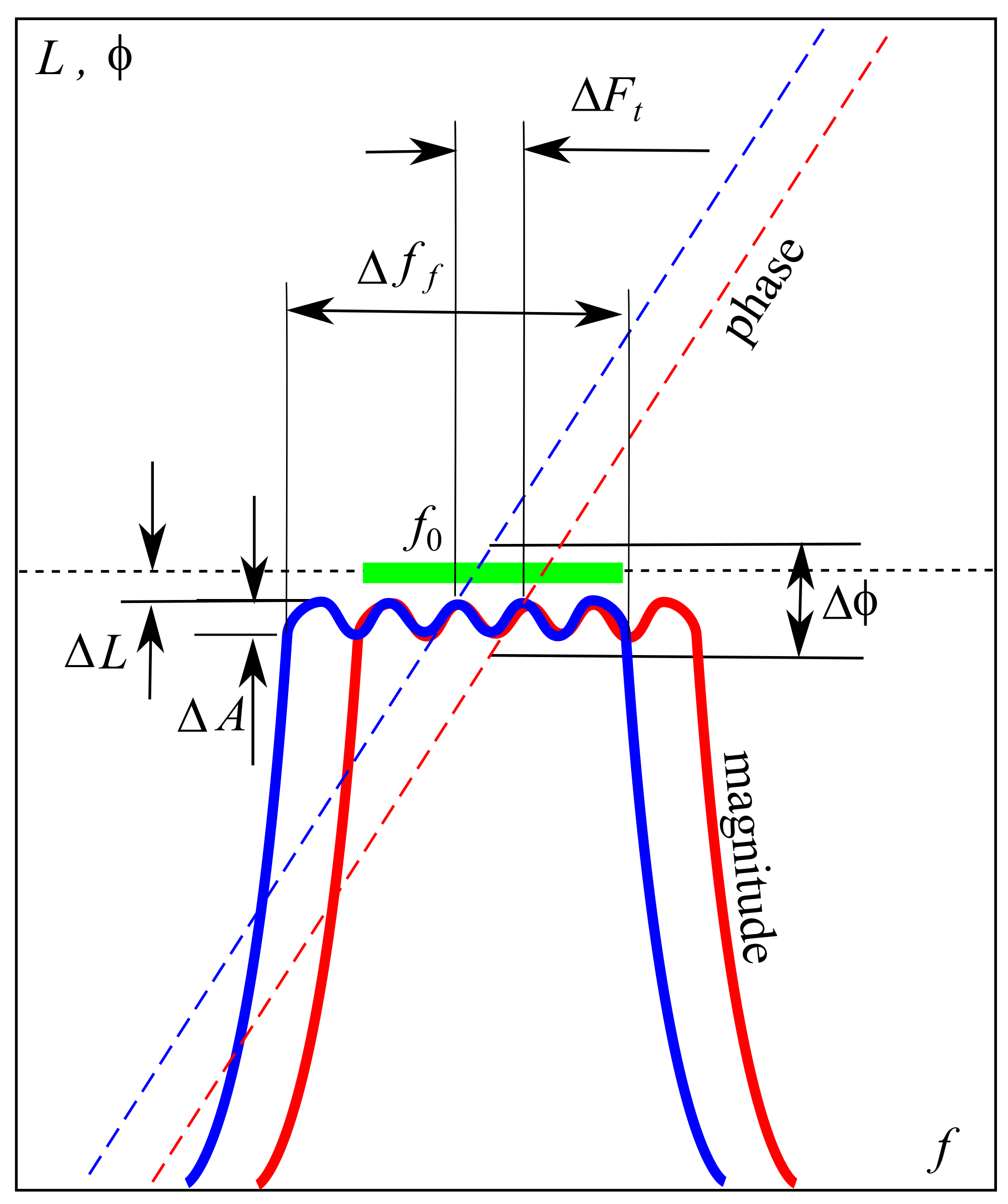
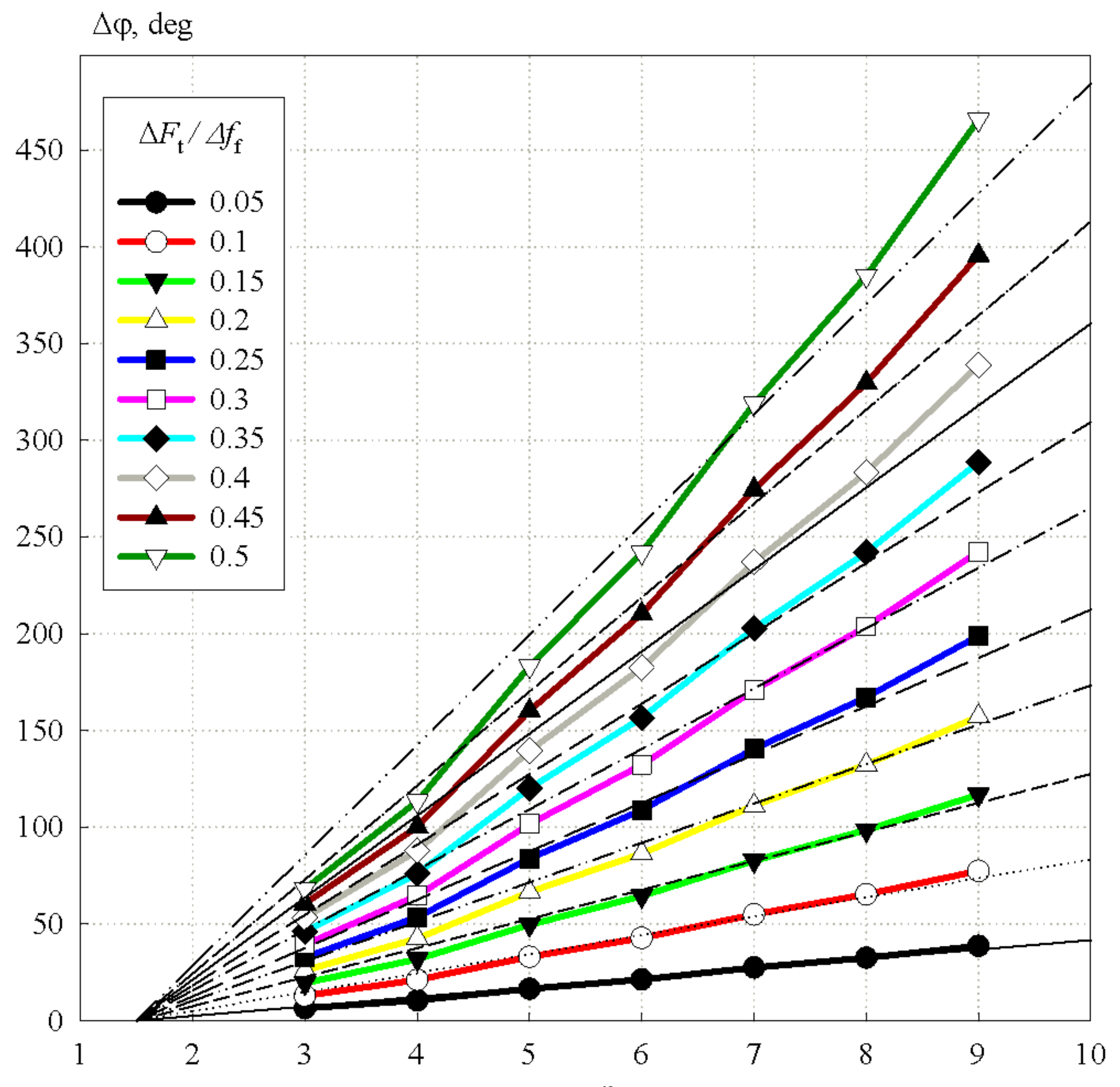
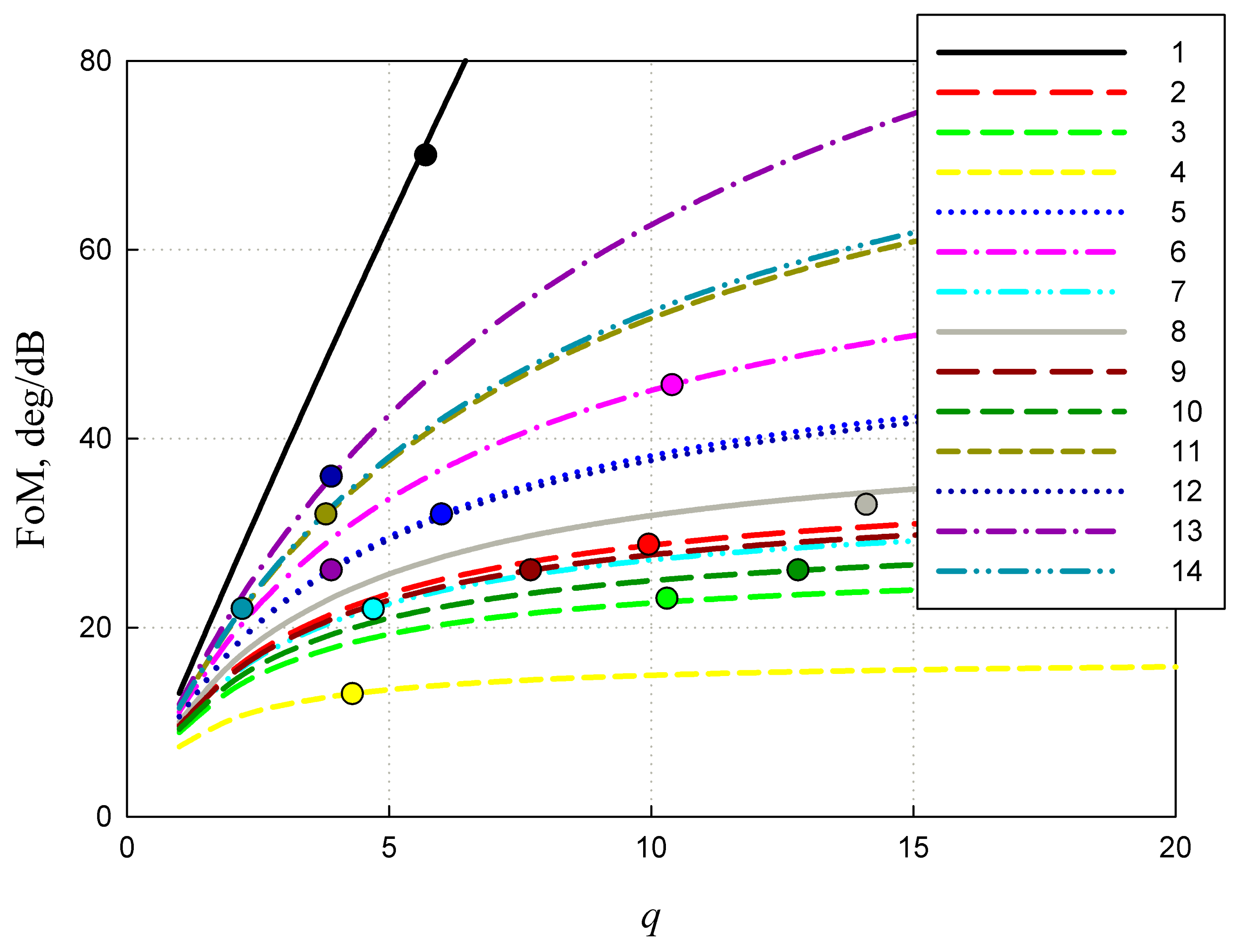
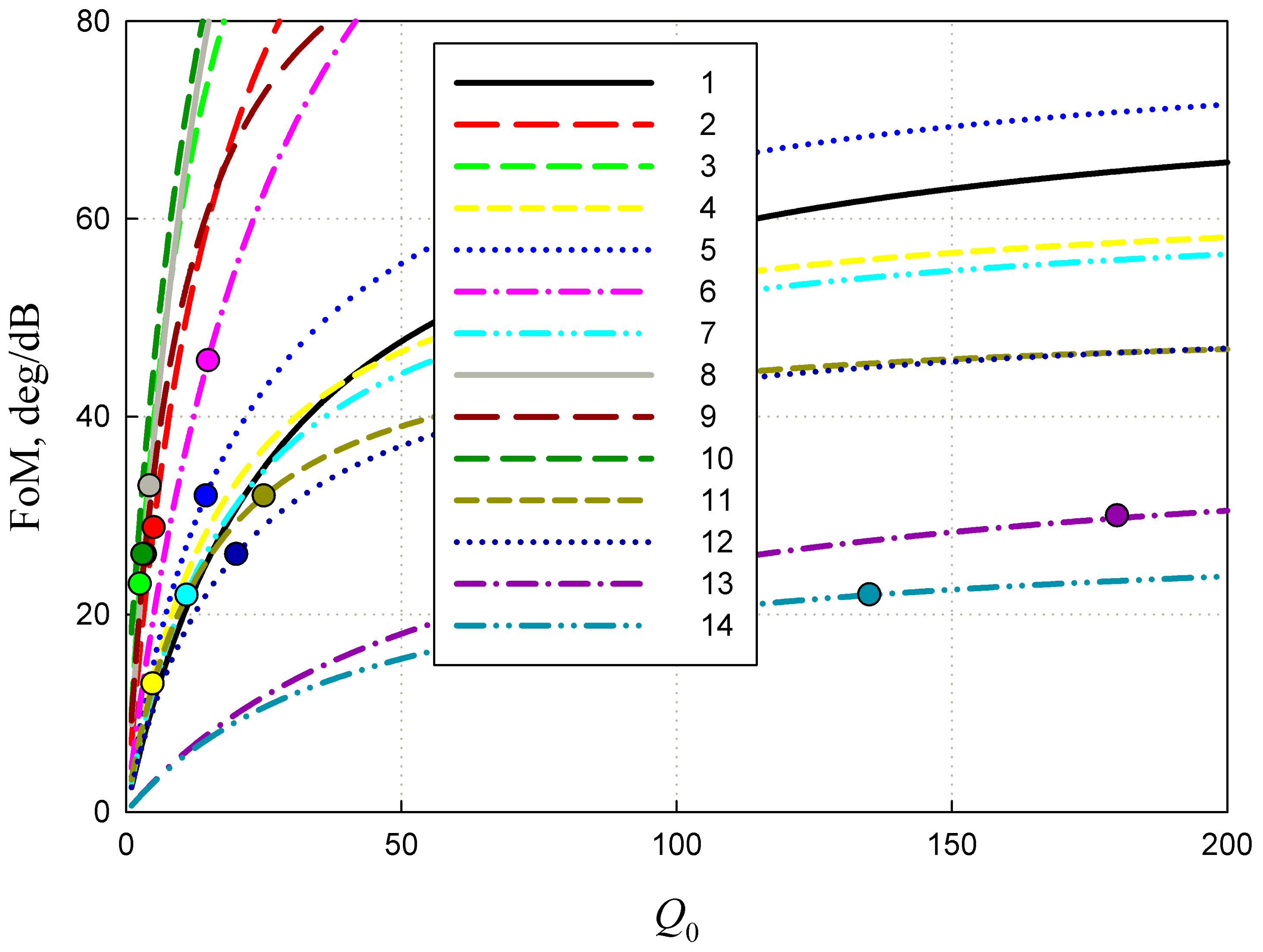
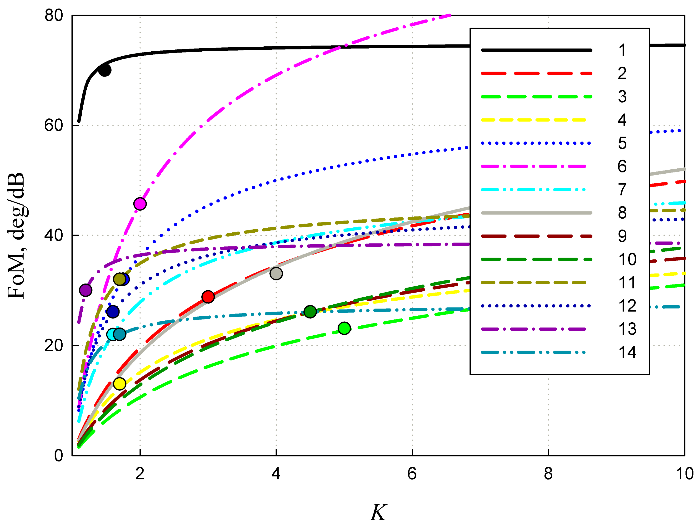
3.1. Comparison of the Figures of Merit for Phase-Shifters Based on the Transmission Line and the Band-Pass Filter

One should note that the phase response of the transmission line-based phase-shifter changes slope with the tuning of the line [14,15,16,17,18,19,20,21,22,23]. It means that the phase-shift difference Δ ϕ is linearly increasing with a frequency (up to the first cut-off frequency in the case of periodically loaded line). At the same time, the group delay is maintained constant versus the frequency (but, of course, is changed with the tuning).
On the other hand, the phase response of the BPF shifts in parallel with the tuning of the filter (see Figure 2). It means that the phase-shift difference Δ ϕ remains constant across the bandwidth of the phase-shifter [24,25,26] and the group delay does not change with the tuning.
It is apparent that the periodically loaded transmission line behaves as a regular one up to the first cut-off frequency and behaves as a band-pass filter at higher pass bands.
Then, let us consider the factor in the definition of line and capacitor figures of merit q line and q that is related to the tunability K. In Figure 4, these factors are plotted versus tunability. One can see that, up to K = 5 , which corresponds to the maximum tunability observed for the FE materials used at microwaves, the factors are equal to each other with a negligible error.
Thus, the figures of merit for the transmission line q line and the capacitor included in resonator q with the constant inclusion coefficient ξ 0 are equal. One can state in this case that q line 2 = q 2 = CQF . In the same way, the term in the insertion loss L that depends on q (second term) is equal for the transmission line based and BPF-based phase-shifters. If the inclusion coefficient ξ is not constant, this statement does not work.
The insertion loss related to the inherent Q-factor in the phase-shifter structure Q 0 (first term in the L definition) depends on tunability—the higher is the tunability, the lower is the loss. Thus, among the capacitors or lines with a similar figure of merit q, the one with higher tunability should be chosen to decrease the insertion loss of the phase-shifter.
The first term in the insertion loss L for the BPF-based phase-shifter contains the inclusion factor ξ 0 < 1 . Thus, the loss related to the inherent Q-factor is higher for this phase-shifter type compared to the one based on a transmission line. If ξ 0 1 , then Equations (11) and (36) become the same. In other words, the inclusion factor for the phase-shifter based on a transmission line is always ξ 0 = 1 .

3.2. Analysis of the Experimental Phase-Shifter

Several published works on the FE based phase-shifter design were reviewed. The parameters of the FE material (capacitors) (k, q and tan δ mean ) and the parameters of the phase-shifters (operating frequency f 0 and figure of merit (FoM)) were extracted. The inclusion factor ξ 0 was supposed to be constant, stated equal to 1 for the transmission line phase-shifters and calculated from the tuning of the filter by Equation (19). The parameters of the model were calculated. Insertion losses for phase-shift of 2 π by Equations (11) and (36) were re-calculated to FoM by Equation (13). The inherent Q-factor Q 0 was calculated as a fitting parameter to approximate the experimental value of FoM with the simulated by the model. The extracted and calculated parameters of reviewed phase-shifters are presented in Table 1.
The figure of merit of the phase-shifters is plotted in Figure 5, Figure 6 and Figure 7 by Equations (11), (13) and (31), using the parameters listed in Table 1, versus figure of merit of capacitor or line q, inherent Q-factor of phase-shifter Q 0 and tunability K. Symbols correspond to the experimental data.
The position of the experimental data point on the calculated curve for the figure of merit allows estimating the importance of the parameter for the design considered. If the experimental point falls on a steep segment of the curve, then improvement of the parameter plotted on the x-axis is of critical importance. If the experimental point falls on the flat segment, the improvement of the parameter is not needed. Analysis of Figure 5, Figure 6 and Figure 7 allows setting a list of improvement priorities for the parameters, as presented in Table 2.

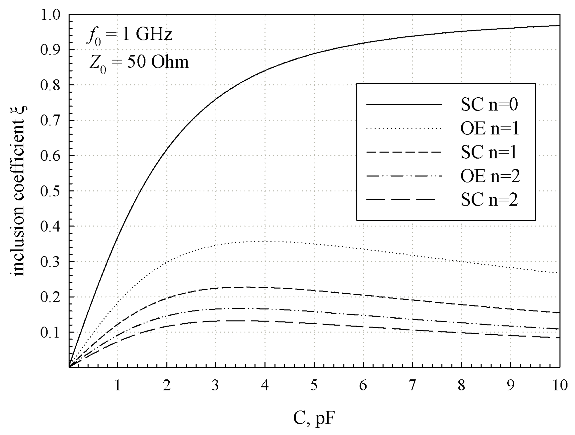
3.3. Suppression of the Amplitude Modulation by the Inclusion Coefficient Control

The behavior of the ferroelectric dielectric loss under the bias voltage application can be different. The loss can decrease [14,27,28] (that is the most common case), remain constant [27] or increase [14]. To suppress the undesirable amplitude modulation in the phase-shifter, one can choose the proper region of the ξ ( C ) dependence (see Appendix B).
Taking into account Equations (A8)–(A11) and (A29), the inclusion coefficient can be plotted versus Z 0 / | X C | (Figure 8), where X C = i / ω 0 C . One can see that the ξ -curves have a maximum corresponding to Z 0 / X C 1 , and there are ascending and descending regions of the dependence (except for the short-circuited resonator with n = 0 ). Parameter n = 0 cannot be set for the open-ended resonator because the resonance condition is not met in this case.
Figure 8 shows that, for example, in the case of decreasing loss tangent under bias, when the capacitance is also decreased (and Z 0 / | X C | as well), one should choose the falling region of the curve ( | X C | < Z 0 ). Therefore, the loss tangent decrease will be compensated by the inclusion coefficient rise, so the Q-factor of the tunable resonator can be kept constant.
If the varying inclusion coefficient is used, then the figure of merit of the tunable capacitor should be calculated by Equation (28).

4. Conclusions

A model of the estimation of the ferroelectric-based phase-shifter figure of merit considering the material properties and phase-shifter design parameters is elaborated.
Closed-form expressions for the insertion loss of the phase-shifter based on FE material are derived considering the two main design approaches: tunable ferroelectric-based transmission line and tunable band-pass filter on the base of FE capacitors. The expressions derived are shown to be quite similar for both approaches. The insertion loss is presented as the sum of the terms depending on the figure of merit of a FE capacitor or transmission line and on the inherent Q-factor of the device without the influence of dielectric loss (or conductive loss only). It is shown that the inherent insertion loss depends on the tunability of a ferroelectric. Thereby, in the case of FE capacitors or lines with equal figures of merit, the one with a greater tunability should be chosen.
The undesirable amplitude modulation in the phase-shifter due to the modulation of dielectric losses is considered. The variation of the inclusion coefficient by the selection of the proper capacitance value is suggested to solve the problem. The special definition of the figure of merit of the tunable capacitor is derived for the case of variating inclusion coefficient.
The published results on FE phase-shifters were reviewed. The figure of merit for the FE capacitor or line was calculated based on the results published. The inherent Q-factor of the device could not be extracted from the review, so it was calculated for all reviewed works as the fitting parameter to equal the insertion loss calculated to the insertion loss published. Dependence of the FE phase-shifters figure of merit on the key parameters of the devices (tunability, figure of merit of the ferroelectric and inherent Q-factor connected to conductive loss) is presented as a basis for the recommendation to the improvement of the devices.

Author Contributions

Conceptualization, A.G. and A.A.; methodology, A.G.; software, A.G.; validation, R.P. and A.A.; formal analysis, A.G.; investigation, T.L.; data curation, T.L.; writing—original draft preparation, A.G.; writing—review and editing, A.A.; visualization, R.P.; supervision, A.A.; project administration, A.A.; and funding acquisition, A.A. All authors have read and agreed to the published version of the manuscript.

Funding

This work was supported by the Russian Science Foundation under grant 18-79-10156.

Institutional Review Board Statement

Not applicable.

Informed Consent Statement

Not applicable.

Data Availability Statement

The data presented in this study are available on reasonable request from the corresponding author.

Acknowledgments

A.G. acknowledges his teacher M. Gaidukov for the beginning of this work and for the analytic skills learned from him.

Conflicts of Interest

The authors declare no conflict of interest.

Appendix A. Inclusion Coefficient and Q-Factor of Resonator

If the microwave resonator consists of a capacitor included into a section of the transmission line, then one can define the parameter that shows what part of the total energy stored in resonator W is stored in the capacitor—the inclusion coefficient:
ξ = W C W C + W line ,
where W C is the energy stored in capacitor, W line is the energy stored in transmission line and W = W C + W line . Then, the quality factor of the capacitor Q C and the quality factor of the whole resonator Q are determined by the energy dissipated in the capacitor W diss C and the energy dissipated in the line W diss line as follows:
Q C = W C W diss C = ξ W W diss C
Q = W W diss C + W diss line .
For the total quality factor of the resonator Q, one can express
1 Q = W diss C W + W diss line W = ξ 1 Q C + 1 Q 0 ,
where Q 0 = W / W diss line is the quality factor of the resonator with lossless capacitor. The quality factor of the capacitor can be expressed as Q C = 1 / tan δ , where tan δ is the effective loss tangent of the capacitor. Thus, the total quality factor of the resonator can be written as
Q = Q 0 1 + ξ Q 0 Q C = Q 0 1 + ξ Q 0 tan δ .

Appendix B. Calculation of Inclusion Coefficient

Appendix B.1. Resonance Conditions

Let us consider the microwave resonator consisting of the capacitor with a capacitance of C included in a transmission line, as depicted in Figure A1. The transmission line has a length of l, a characteristic impedance of Z 0 , a propagation constant of β 0 and is loaded onto the termination load with an impedance of Z load .
Figure A1. Electrical equivalent circuit of the resonator including a capacitor and a section of a transmission line.
Crystals 11 00538 g0a1
The load impedance is transformed to the position of the capacitor ( z = 0 ) according to the well-known impedance transformation formula
Z ( z ) = Z 0 Z load + i Z 0 tan ( β 0 l ) Z 0 + i Z load tan ( β 0 l ) ,
so the resonance condition at a resonance frequency of ω 0 can be written as
X C = i ω 0 C 1 = Z ( l ) ,
where X C is the impedance of the capacitance.
One can suggest that the load condition of the line can be a short-circuit ( Z load = 0 ) or an open-end ( Z load = ), thus the resonance conditions are as follows:
C = 1 ω 0 Z 0 cot β 0 l ,
C = 1 ω 0 Z 0 tan β 0 l ,
where Equation (A8) corresponds to short-circuit and Equation (A9) corresponds to open-end.
The argument of the trigonometric functions in Equations (A8) and (A9) can be referred to as the electrical length (or phase length) of the section of the transmission line at the resonance measured in radians:
ϕ = β 0 l = arctan | X C | Z 0 + π n , n = 1 , 2 ,
ϕ = β 0 l = arctan Z 0 | X C | + π n , n = 1 , 2 ,
At the frequency of resonance ω 0 , the propagation constant can be defined as
β 0 = ω 0 v = 2 π Λ 0
where v = μ ε 1 is the light velocity in the transmission line, μ and ε are effective permeability and permittivity of the line and Λ 0 is the wavelength in the line at the resonance frequency.

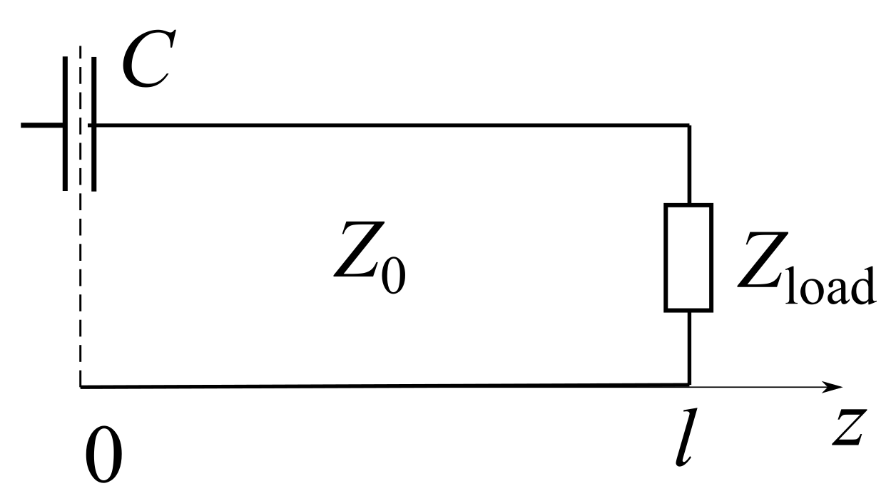
Appendix B.2. Energy Stored in the Transmission Line Section

Let us consider the regular TEM-mode transmission line. The cross-section of the simplest line—the parallel-plane line—is presented in Figure A2.
Figure A2. Cross-section of the simplest transmission line.
Crystals 11 00538 g0a2
The characteristic impedance of the line in Figure A2 can be defined as
Z 0 = L 0 C 0 ,
where L 0 = μ l d w is the inductance of the line and C 0 = ε w l d is the capacitance of the line. Thus, the impedance can be written as
Z 0 = μ l d w d ε w l ε ε .
Accounting for the light velocity v, one can state that
w ε d = 1 Z 0 v .
The energy stored in the transmission line section with the length l is defined as
W line = 1 2 V ε E 2 d V ,
where V is the volume of the line and E is the electric field strength. For the line considered V = w d l and E = U / d , where U is the voltage in the TEM-mode line. Since the line is regular, d V = w d d z and Equation (A16) can be written as
W line = ε 2 w d 0 l U ( z ) 2 d z .
The distribution of the voltage along the transmission line (starting from the line end) is defined as
U ( z ) = U max sin β 0 z = U max sin β 0 z ,
U ( z ) = U max cos ( β 0 z ) = U max cos ( β 0 z ) ,
where U max is the amplitude of the microwave signal.
Thus, the energy stored in the line is
W line = ε w 2 d U max 2 0 l sin 2 ( β 0 z ) d z = ε w 4 d U max 2 l 1 2 β 0 sin 2 β 0 l = U max 2 4 1 Z 0 v l 1 sin ( 2 β 0 l ) 2 β 0 l ,
W line = ε w 2 d U max 2 0 l cos 2 ( β 0 z ) d z = U max 2 4 1 Z 0 v l 1 + sin ( 2 β 0 l ) 2 β 0 l ,

Appendix B.3. Energy Stored in the Capacitor

Energy stored in the capacitor is defined as
W C = C U C 2 2 ,
where U C is the voltage across the capacitor.
For the short-circuited transmission line, the voltage is
U C = U m sin ( β 0 l ) ,
and, for the open-ended transmission line, it is
U C = U m cos ( β 0 l ) .
Substituting Equations (A23) and (A24) into Equation (A22), and taking into account Equations (A8) and (A9), one can write for the short-circuited and open-ended lines respectively
W C = 1 2 U C 2 1 ω 0 Z 0 cot β 0 l sin 2 ( β 0 l ) = 1 4 U C 2 1 ω 0 Z 0 sin ( 2 β 0 l )
W C = 1 2 U C 2 1 ω 0 Z 0 tan β 0 l cos 2 ( β 0 l ) = 1 4 U C 2 1 ω 0 Z 0 sin ( 2 β 0 l )

Appendix B.4. Inclusion Coefficient

Substituting Equations (A20), (A21) and (A25), (A26) into Equation (A1), one can write for the inclusion coefficients of the short-circuited and open-ended resonators, respectively,
ξ = 2 1 + 2 β 0 l sin ( 2 β 0 l )
ξ = 2 1 2 β 0 l sin ( 2 β 0 l )
It can be shown that, if the capacitance versus resonance frequency dependence is known, for example, if it is defined by Equations (A8) and (A9), then the inclusion coefficient (Equations (A27) and (A28)) can be calculated as follows:
ξ = 2 C ω 0 d ω 0 d C
Equation (A29) is also valid when the dependence of a capacitance on a resonant frequency is defined in any other way, for example, by polynomial approximation of the experimental data.

References

  1. Vendik, O.G.; Carlsson, E.F.; Petrov, P.K.; Chakalov, R.A.; Gevorgian, S.S.; Ivanov, Z.G. HTS/Ferroelectric CPW Structures for Voltage Tuneable Phase Shifters. In Proceedings of the 1997 27th European Microwave Conference, Jerusalem, Israel, 8–12 September 1997; Volume 1, pp. 196–202. [Google Scholar] [CrossRef]
  2. Vendik, I.B.; Vendik, O.G.; Kollberg, E.L. Criterion for a Switching Device as a Basis of Microwave Switchable and Tunable Components. In Proceedings of the 1999 29th European Microwave Conference, Munich, Germany, 5–7 October 1999; Volume 3, pp. 187–190. [Google Scholar] [CrossRef]
  3. Vendik, O.; Hollmann, E.; Kozyrev, A.; Prudan, A. Ferroelectric tuning of planar and bulk microwave devices. J. Supercond. 1999, 12, 325–338. [Google Scholar] [CrossRef]
  4. Vendik, I.B.; Vendik, O.G.; Kollberg, E.L. Commutation quality factor of two-state switchable devices. IEEE Trans. Microw. Theory Tech. 2000, 48, 802–808. [Google Scholar] [CrossRef]
  5. Vendik, O.G.; Vendik, I.B.; Sherman, V.O. Commutation Quality Factor as a Working Tool for Optimization of Microwave Ferroelectric Devices. Integr. Ferroelectr. 2002, 43, 81–89. [Google Scholar] [CrossRef]
  6. Buslov, O.Y.; Keis, V.N.; Kotelnikov, I.V.; Golovkov, A.A.; Sugak, M.I.; Kozyrev, A.B.; Sengupta, L. Slot-Line Ferroelectric Phase-Shifters and Phase-Array Antenna On Their Base. Integr. Ferroelectr. 2006, 86, 125–130. [Google Scholar] [CrossRef]
  7. Buslov, O.Y.; Keis, V.N.; Kotelnikov, I.V.; Kozyrev, A.B.; Tumarkin, A.V. Microwave Ferroelectric Phase Shifters Based on the Periodical Structures. In Proceedings of the 2006 IEEE MTT-S International Microwave Symposium Digest, San Francisco, CA, USA, 11–16 June 2006; pp. 1269–1272. [Google Scholar] [CrossRef]
  8. Sherman, V.; Astafiev, K.; Setter, N.; Tagantsev, A.; Vendik, O.; Vendik, I.; Hoffmann-Eifert, S.; Bottger, U.; Waser, R. Digital reflection-type phase shifter based on a ferroelectric planar capacitor. IEEE Microw. Wirel. Compon. Lett. 2001, 11, 407–409. [Google Scholar] [CrossRef]
  9. Kozyrev, A.; Buslov, O.; Keis, V.; Dovgan, D.; Kotelnikov, I.; Kulik, P.; Sengupta, L.; Chiu, L.; Zhang, X. 14 GHz Tunable Filters Base on Ferroelectric Films. Integr. Ferroelectr. 2003, 55, 905–913. [Google Scholar] [CrossRef]
  10. Vendik, O.G.; Vendik, I.B.; Pleskachev, V.V. Figure of Merit of Tunable Ferroelectric Planar Filters. Integr. Ferroelectr. 2003, 55, 973–981. [Google Scholar] [CrossRef]
  11. Maloratsky, L. Passive RF and Microwave Integrated Circuits; Elsevier: Amsterdam, The Netherlands, 2003; p. 8. [Google Scholar]
  12. Kozyrev, A.; Keis, V.; Koepf, G.; Yandrofski, R.; Soldatenkov, O.; Dudin, K.; Dovgan, D. Procedure of microwave investigations of ferroelectric films and tunable microwave devices based on ferroelectric films. Microelectron. Eng. 1995, 29, 257–260. [Google Scholar] [CrossRef]
  13. Matthaei, G.L.; Young, L.; Jones, E.M.T. Microwave Filters, Impedance-Matching Networks, and Coupling Structures; Artech House: Norwood, MA, USA, 1980. [Google Scholar]
  14. Kozyrev, A.; Keis, V.; Osadchy, V.; Pavlov, A.; Buslov, O.; Sengupta, L. Microwave properties of (Ba, Sr) TiO3 ceramic films and phase-shifters on their base. Integr. Ferroelectr. 2001, 34, 189–195. [Google Scholar] [CrossRef]
  15. Lee, S.; Ryu, H.; Moon, S.; Kwak, M.; Kim, Y.; Kang, K. X-band ferroelectric phase shifter using voltage-tunable (Ba, Sr) TiO3 varactors. J. Korean Phys. Soc. 2006, 48, 1286–1290. [Google Scholar]
  16. De Paolis, R.; Coccetti, F.; Payan, S.; Maglione, M.; Guegan, G. Characterization of ferroelectric BST MIM capacitors up to 65 GHz for a compact phase shifter at 60 GHz. In Proceedings of the 2014 IEEE 44th European Microwave Conference, Rome, Italy, 6–9 October 2014; pp. 492–495. [Google Scholar]
  17. Velu, G.; Burgnies, L.; Houzet, G.; Blary, K.; Lippens, D.; Carru, J. Characterization of ferroelectric films up to 60 GHz: Application to phase shifters. Integr. Ferroelectr. 2007, 93, 110–118. [Google Scholar] [CrossRef]
  18. Sheng, S.; Wang, P.; Chen, X.; Zhang, X.Y.; Ong, C. Two paralleled Ba 0.25 Sr 0.75 TiO3 ferroelectric varactors series connected coplanar waveguide microwave phase shifter. J. Appl. Phys. 2009, 105, 114509. [Google Scholar] [CrossRef]
  19. Acikel, B.; Liu, Y.; Nagra, A.S.; Taylor, T.R.; Hansen, P.J.; Speck, J.S.; York, R.A. Phase shifters using (Ba, Sr) TiO3 thin films on sapphire and glass substrates. In Proceedings of the 2001 IEEE MTT-S International Microwave Sympsoium Digest (Cat. No. 01CH37157), Phoenix, AZ, USA, 20–24 May 2001; Volume 2, pp. 1191–1194. [Google Scholar]
  20. Ryu, H.C.; Moon, S.E.; Lee, S.J.; Kwak, M.H.; Kim, Y.T. Microwave performance of distributed analog phase shifter using ferroelectric (Ba, Sr) TiO3 thin films. Integr. Ferroelectr. 2003, 54, 689–696. [Google Scholar] [CrossRef]
  21. Annam, K.; Spatz, D.; Shin, E.; Subramanyam, G. Experimental Verification of Microwave Phase Shifters Using Barium Strontium Titanate (BST) Varactors. In Proceedings of the 2019 IEEE National Aerospace and Electronics Conference (NAECON), Dayton, OH, USA, 15–19 July 2019; pp. 63–66. [Google Scholar]
  22. Mercier, D.; Niembro-Martin, A.; Sibuet, H.; Baret, C.; Chautagnat, J.; Dieppedale, C.; Bonnard, C.; Guillaume, J.; Le Rhun, G.; Billard, C.; et al. X band distributed phase shifter based on sol-gel BCTZ varactors. In Proceedings of the IEEE 2017 European Radar Conference (EURAD), Nuremberg, Germany, 11–13 October 2017; pp. 382–385. [Google Scholar]
  23. Kozyrev, A.; Gaidukov, M.; Gagarin, A.; Tumarkin, A.; Razumov, S. A finline 60-GHz phase shifter based on a (Ba, Sr) TiO3 ferroelectric thin film. Tech. Phys. Lett. 2002, 28, 239–241. [Google Scholar] [CrossRef]
  24. Sazegar, M.; Mehmood, A.; Zheng, Y.; Maune, H.; Zhou, X.; Binder, J.; Jakoby, R. Compact tunable loaded line phase shifter based on screen printed BST thick film. In Proceedings of the IEEE 2011 German Microwave Conference, Darmstadt, Germany, 14–16 March 2011; pp. 1–4. [Google Scholar]
  25. Deleniv, A.; Abadei, S.; Gevorgian, S. Tunable ferroelectric filter-phase shifter. In Proceedings of the IEEE MTT-S International Microwave Symposium Digest, Philadelphia, PA, USA, 8–13 June 2003; Volume 2, pp. 1267–1270. [Google Scholar]
  26. Kozyrev, A.; Ivanov, A.; Soldatenkov, O.; Tumarkin, A.; Razumov, S.; Aigunova, S.Y. Ferroelectric (Ba, Sr) TiO3 Thin-Film 60-GHz Phase Shifter. Tech. Phys. Lett. 2001, 27, 1032–1034. [Google Scholar] [CrossRef]
  27. Su, B.; Holmes, J.; Meggs, C.; Button, T. Dielectric and microwave properties of barium strontium titanate (BST) thick films on alumina substrates. J. Eur. Ceram. Soc. 2003, 23, 2699–2703. [Google Scholar] [CrossRef]
  28. Borderon, C.; Ginestar, S.; Gundel, H.W.; Haskou, A.; Nadaud, K.; Renoud, R.; Sharaiha, A. Design and Development of a Tunable Ferroelectric Microwave Surface Mounted Device. IEEE Trans. Ultrason. Ferroelectr. Freq. Control 2020, 67, 1733–1737. [Google Scholar] [CrossRef] [PubMed]
Figure 1. The dependence of the inclusion coefficient on capacitance value.
Crystals 11 00538 g001
Figure 2. Frequency response of the phase shifter based on the band-pass filter.
Crystals 11 00538 g002
Figure 3. Phase shift versus the number of resonators.
Crystals 11 00538 g003
Figure 4. Tunability-related factor versus tunability.
Crystals 11 00538 g004
Figure 5. Figure of merit of phase-shifter versus figure of merit of capacitor or line.
Crystals 11 00538 g005
Figure 6. Figure of merit of phase-shifter versus inherent Q-factor.
Crystals 11 00538 g006
Figure 7. Figure of merit of phase-shifter versus tunability.
Crystals 11 00538 g007
Figure 8. Inclusion coefficient versus Z 0 / X C .
Crystals 11 00538 g008
Table 1. Experimental parameters of phase-shifters reviewed.
#RefType f 0 , GHz tan δ mean KqFoM, deg/dB ξ 0 Q 0
1[14]regular300.0351.485.7701500
2[15]loaded100.5639.9528.715
3[16]loaded650.08510.32312.5
4[17]loaded300.0621.74.31314.8
5[18]loaded200.0471.75632114.5
6[19]loaded200.33210.445.7114.9
7[20]loaded100.051.64.722111
8[21]loaded120.05414.13314.3
9[22]loaded120.014.57.72613.45
10[17]loaded300.064.512.82613.0
11[23]regular600.071.73.832125
12[24]filter100.061.63.9260.8520
13[25]filter200.031.23300.55180
14[26]loaded600.121.72.2220.19135
Table 2. Priorities to improve the phase-shifter parameters.
#RefType f 0 , GHzMust Be ImprovedMay Be ImprovedNo Need to Improve
1[14]regular30q- K , Q 0
2[15]loaded10 Q 0 Kq
3[16]loaded65 Q 0 Kq
4[17]loaded30 Q 0 , K q-
5[18]loaded20 Q 0 , K q-
6[19]loaded20 Q 0 , K q-
7[20]loaded10 Q 0 , K -q
8[21]loaded12 Q 0 , K -q
9[22]loaded12 Q 0 Kq
10[17]loaded30 Q 0 Kq
11[23]regular60q Q 0 , K -
12[24]filter10 Q 0 , K q-
13[25]filter20 q , K - Q 0
14[26]loaded60q- Q 0 , K
Publisher’s Note: MDPI stays neutral with regard to jurisdictional claims in published maps and institutional affiliations.

