Deep Neural Networks for Analysis of Microscopy Images—Synthetic Data Generation and Adaptive Sampling

Abstract

The analysis of microscopy images has always been an important yet time consuming process in materials science. Convolutional Neural Networks (CNNs) have been very successfully used for a number of tasks, such as image segmentation. However, training a CNN requires a large amount of hand annotated data, which can be a problem for material science data. We present a procedure to generate synthetic data based on ad hoc parametric data modelling for enhancing generalization of trained neural network models. Especially for situations where it is not possible to gather a lot of data, such an approach is beneficial and may enable to train a neural network reasonably. Furthermore, we show that targeted data generation by adaptively sampling the parameter space of the generative models gives superior results compared to generating random data points.

1. Introduction

Microscopy image analysis has been strongly intertwined with materials science and has helped for more than a century to understand the relationship between structural or atomic aspects and the respective materials’ properties. Typical workflows for image analysis include segmentation of, e.g., different phases or defects. This is usually done by manually labeling the images followed by counting the occurrences of, e.g., inclusions or through characterizing geometrical features of the phases or defects. This is not only a tedious process, but also requires expert knowledge, thus, a certain amount of human bias is always included.

Image processing—not only in materials science or microscopy—has tremendously benefited from deep learning (DL) ever since the seminal work of Krizhevsky et al. [1] in 2012. A variety of improved deep neural networks have been developed subsequently, such as ResNet (He et al. [2]) for classification or U-Net (Ronneberger et al. [3]) for segmentation. However, all neural networks published so far are essentially useless for solving real-world problems without the availability of appropriate training data. This has been partially remedied by open source databases of already labeled images. The most prominent example is ImageNet (Deng et al. [4]) containing over 14 million annotated images of thousands of object classes (e.g., plants, geological formations, tools, artifacts, animals or persons) and their sub-classes. However, if the feature to be segmented or classified is not contained in available datasets (e.g., a micrograph of a phase or grain microstructure from a scanning electron microscope), training models based on images of such databases generally leads to a poor prediction accuracy.

A remedy of this dilemma occurred when Yosinski et al. [5] identified the phenomenon that first layer features of neural networks trained on natural images are not specific to a dataset or task. As a consequence, once learned on a dataset, these features can be reused in a different context. Additionally, also mid-level features in later layers turned out to be similar. This has a high relevance also for microscopy in materials science: microscopy images of a grain boundary and for example a contour of a house both contain as common features straight line segments, and possibly even circular or elliptical features. Thus, transferring features learned on big but unrelated datasets to other, possibly specialized fields of applications has become a standard approach since then and is called transfer learning (Shin et al. [6]). Unfortunately, at least the fully connected parts of the network must still be trained from scratch (at least when unknown classes are contained). Nonetheless, also materials science, and in particular microsopcy, has already significantly benefitted from these developments, as is evident from a growing body of literature [7,8,9,10]. In such a case, using hand-labeled datasets for training during transfer learning still may require a significant number of high-quality, hand-labeled images, but incorporating transfer learning is already considerably faster than manual image segmentation and analysis: in [11] the authors demonstrated that for classification of five different types of damage in micrographs of a dual-phase steel, a human would require ≈6 h for analysis of the approximately 1000 damage sites contained in a large, panoramic image, while DL-based prediction takes a negligible amount of time with initially ≈25 h for labeling and 3 h for learning. If the features become more complicated or more classes of different features should be recognized substantially more training data must be provided. The same also applies in other communities, Cordts et al. [12] presented an example where high-level manual semantic labeling required more than 90 min per image on average, which means over 7500 h for their whole dataset. Annotating such a vast amount of data is very tedious and also usually requires experts’ experience for obtaining high-quality training data.

Tools developed to assist the annotation process, such as LabelMe (Russell et al. [13]) or Polygon-RNN++ (Acuna et al. [14]) should facilitate the process. Nevertheless, the curse of dataset annotation as stated by Xie et al. [15] remains one of the biggest challenges, as such tools often only work when similar data had already been annotated. Besides annotation, it can be very expensive and time consuming to generate a data point which may restrict the maximal number of images to be collected. Rare and diverse events pose a further problem where it is not possible to do experiments to collect more data. A phenomenon may even be known only theoretically, which means it has not been observed yet in real data, but it is known how the phenomenon should appear based on physics. In this case it is impossible to train a model based on real data.

When provided with a too small dataset for training the resulting models often suffer from overfitting leading to a lack of generalization. Regularization methods such as dropout (Srivastava et al. [16]), batch normalization ([17,18]), or weight decay (Krogh et al. [19]) can help to reduce the amount of overfitting. However, regularization does not help to increase the amount of available data. Data augmentation approaches ([20,21]) try to overcome this problem by adding transformed versions of the original data to the dataset. Vasconcelos et al. [22], for example, used classical image transforms and image warping techniques for training a skin cancer detection model. This approach was supported by domain experts for generating additional realistic versions of available images.

Besides data augmentation, approaches using synthetic data have been proposed as well. Richter et al. [23] extracted 25,000 images from a photorealistic open-world computer game. By utilizing the source code to generate dense pixel-level semantic annotations they generated training data and showed that the additional data could enhance model performance. Goodfellow et al. [24] proposed Generative Adversarial Networks, a neural network architecture that is capable of generating artificial data from noise, e.g., to synthesize fake images of faces (Karras et al. [25]). Shao et al. [26] presented such a generative model for signal data augmentation to diagnose machine faults.

Poibrenski et al. [27] demonstrated in a bounded setting that synthetic data can enhance the ability to detect pedestrians in an autonomous driving scenario. Tremblay et al. [28] presented a system applying domain randomization to generate non-realistic augmented images. This procedure should force the neural network to learn essential features of objects of interest. They evaluated the method on object detection with bounding boxes and showed the positive impact of the addition of synthetic data during training. Deep domain adaptation is a further option to tackle the non-availability of data, respectively, labels. See the survey from Wang and Deng [29] for more information. Deep domain adaptation methods take care that neural networks learn more transferable representations by embedding domain adaptation techniques into the training loop (Sun and Saenko [30]). Besides defining a taxonomy for such methods, the authors give an overview of computer vision applications that use such techniques.

We propose to use parametric models of materials science phenomena in combination with forward simulations of a measurement process to generate synthetic data for training neural networks. The approach provides a way to apply supervised learning methods in situations where the availability of training data poses a problem. This is the case (i) if the generation requires expensive measurement equipment or sample preparations, (ii) if the generation of training data involves ethical concerns, (iii) if the manual labeling constitutes an infeasible effort, or (iv) if a phenomenon has been predicted but not yet observed, i.e., training data is unavailable [31]. Synthetic training data generation poses an elegant and straightforward solution to all class imbalance and data imbalance problems.

We demonstrate our approach for two use cases that underlie different assumptions for the parametric models and the corresponding synthetic data generation incorporating classification and segmentation. The first example is concerned with surface crack detection where statistical measurements and texture generation are used for the synthetic data creation. The second example is the synthetic data generation of grain boundaries, which only relies on the visual appearance of available samples. For each example we explain the parametric model and the related data generation, train a neural network based on the synthetic data, apply fine tuning with real data if possible, and evaluate the performance of the learned models to show the usefulness of our approach.

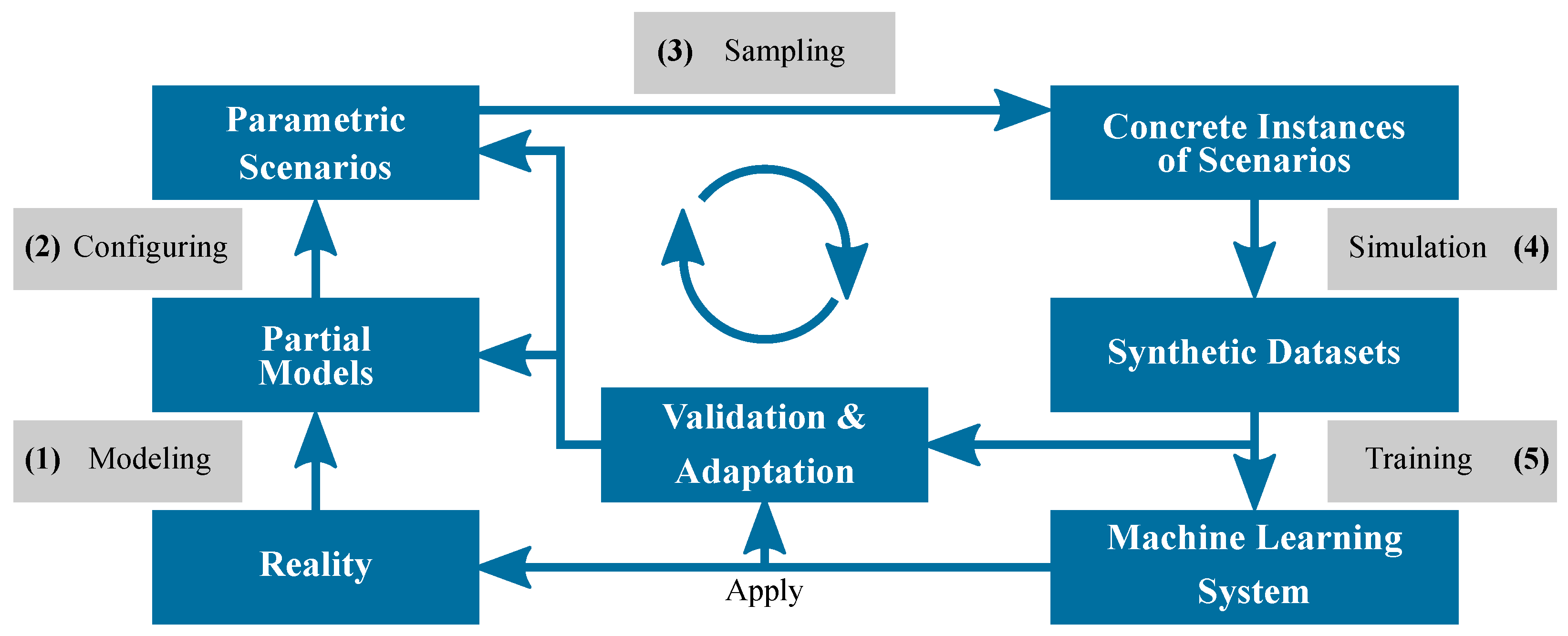
2. Materials and Methods

2.1. Synthetic Training Data

Our approach relies on a concept called ’partial models’ of the world. Partial models are parametric in the sense that each model is controlled by a number of input parameters. Examples are the specific aspects of the world that we are interested in, for example the (average) grain size or possible configurations of surface defects such as cracks. The partial models jointly represent a real world configuration and form a generative model. Each setting of the parameters constitutes one scenario. Using forward simulation of a measurement process, synthetic data can be generated (Figure 1).

Partial models can be acquired via capturing (e.g., from 3D rendering as investigated in Su et al. [32]) or manual creation. We exclusively focus on the latter, i.e., procedural generation using data driven 2D models. This typically involves obtaining a deeper understanding of aspects of reality independent from the learning process. Models may describe full real world effects. Here, we concentrate on ’shallow’ models which are models that are described in phenomenological terms and that use procedures based on abstractions of the real world. As opposed to a physical simulation, such models are not based on the underlying physical relationships of a phenomenon but only mimic the results. This often suffices for the generation of training data; as compared to realistic, physical simulations, this has clear benefits in terms of method complexity and computational cost. Such partial models also reduce the high-dimensional parameter spaces inherent to physical models of the real world.

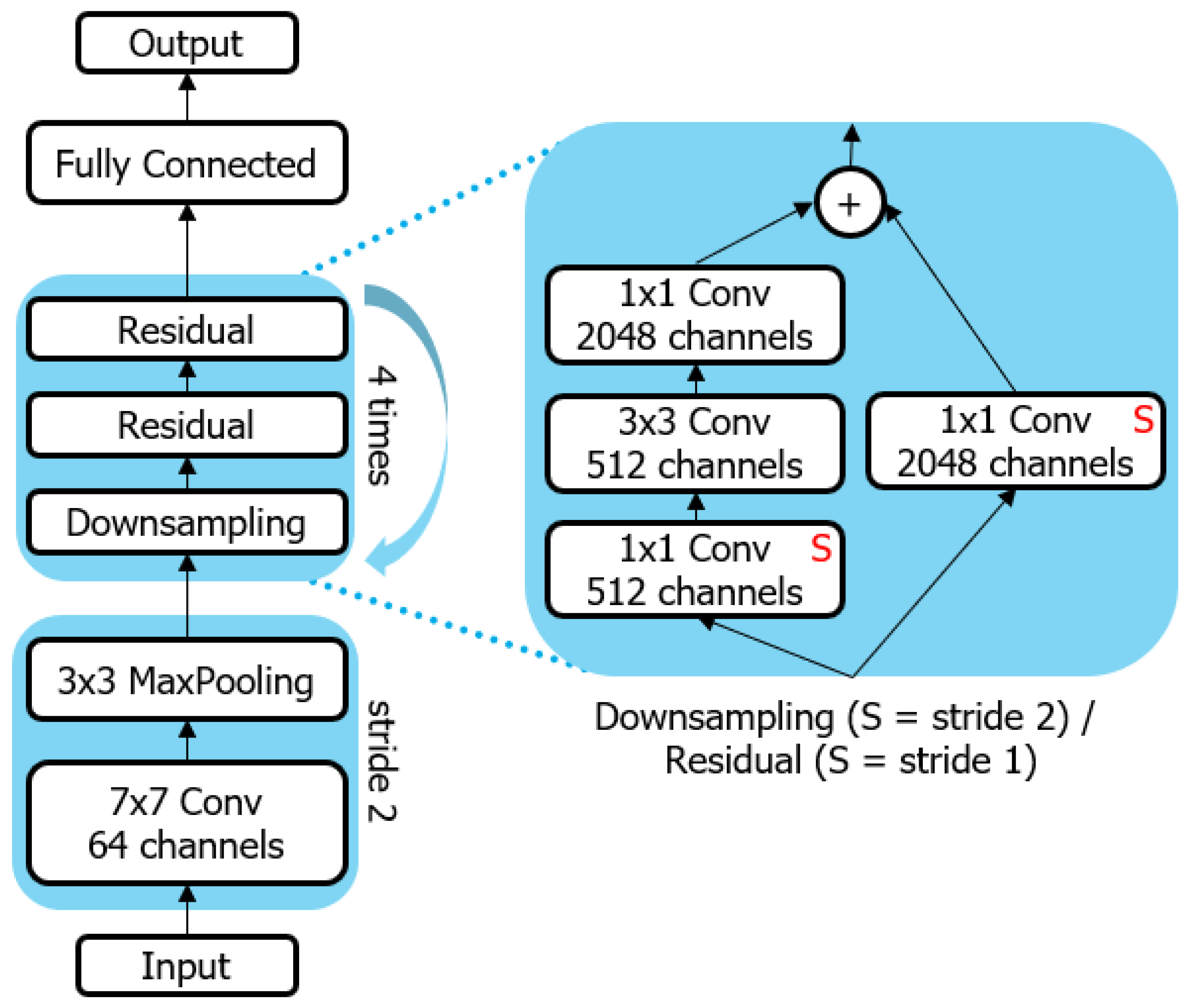
2.2. Machine Learning Setup

In the following we conduct two use case studies for different scenarios to show the effectiveness of synthetic data generated based on parametric models to enhance training performance of neural networks. We unified most of the training procedure for both use cases and trained the models using FastAI library [33] (Version 1.0.51). Here, we describe the general procedure that both training procedures have in common. Deviations are elucidated for each use case separately in the corresponding section. As computing infrastructure we use a server with Ubuntu 18.04 that contains two Nvidia Tesla V100 with 32 GB RAM each and 40 hyper-threaded Intel Xeon(R) CPU E5-2630 v4 cores with $2.20$ GHz.

For classification we use a ResNet50, i.e., the used architecture has 50 layers (He et al. [2]), as shown in Figure 2, for segmentation we use a ResNet50 based U-Net (Ronneberger et al. [3]). That means the original U-Net architecture is adapted, so that standard convolutional layers are replaced by residual blocks as shown in Figure 2 and, furthermore, ResNet50 is used as backbone of the hourglass-like U-Net architecture for the segmentation process. All trainings are performed with a pretrained ImageNet (Deng et al. [4]) utilizing transfer learning (Yosinski et al. [5]) and the FastAI defaults. We adapted the pretrained models by replacing the fully connected part with a custom part, also called head, adapted to the individual use case. We first trained the custom part without altering the pretrained parts. We then made the whole network trainable and conducted a further training. The exact numbers for varying hyperparameters can be found in each use case.

For all experiments the synthetic data was divided into training and validation set. As we were not interested in evaluating the generalization on synthetic images, we did not use a test set for the synthetic data. Instead, real data was used as test set for assessing model quality. In addition to the synthetic image generation via parametric modelling we used data augmentation whenever meaningful, e.g., to simulate different lighting conditions, zooming, or rotations. Learning rates were selected based on a cyclical learning rate scheduler and the learning rate finder described in Smith [34]. We did not perform any further parameter tuning. We run each scenario 200 times with different random partitioning of training and validation set. For being able to reproduce the experiments, we set the random seed in each run to the corresponding number of the run from 1 to 200. Based on these runs we computed the mean value ± standard deviation of the applied evaluation metric as well as $99\%$ confidence intervals according to Agresti and Coull [35]. For classification we used an error rate, which is defined as wrong classifications divided by all classifications. For segmentation we additionally used mean pixel intersection over union of all classes (compare Long et al. [36]), which is defined per class as the intersection of the ground truth and the prediction divided by the union of both. Furthermore, we conducted a paired two-tailed t-test (Zabell [37]) for the null hypothesis that mean errors are equal when it was possible to train a model on real data. A p-value below $0.05$ led to rejecting this hypothesis, which means there is a statistically significant difference.

3. Results

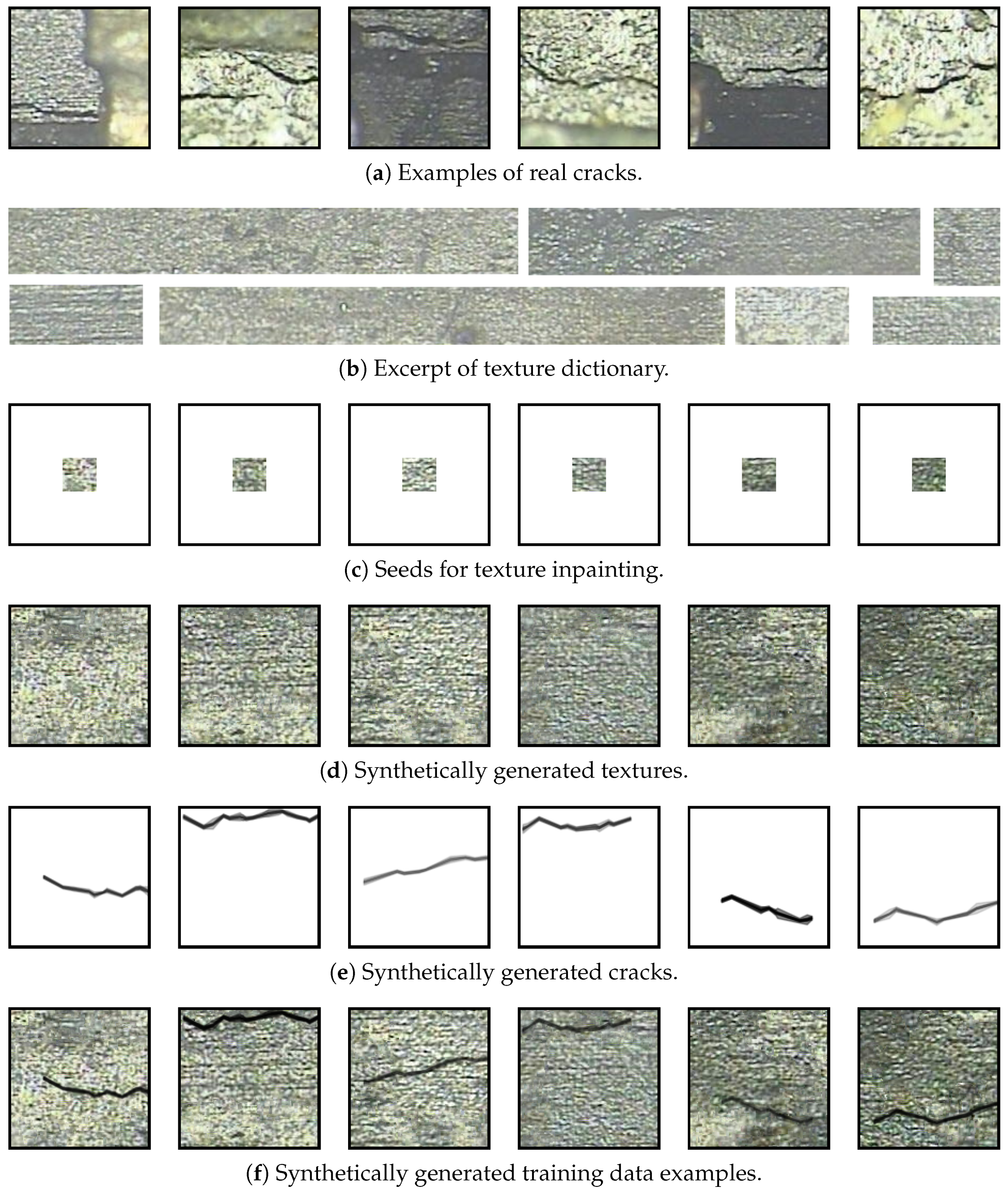
3.1. Surface Crack Detection during Optical Screening

Identification of surface cracks on a sample of material during testing or during manufacturing of work pieces is an important process that gives insight into failure modes or that helps to maintain a high quality during production. There, screening out faulty work pieces as early as possible increases production output as less time is wasted on their further processing. We want to automate the inspection of material samples (here: electronic chips) to detect surface cracks that would disturb the normal operation of the chip (here: cracks in the protective housing). A deep neural network should be trained to classify excerpts of a chip as faulty, which means containing a crack, or error-free. A trained model should be able to work on a wide range of similar samples, which in this case means different chips: rather than learning one particular sample and the occurring deviations, the model must learn to detect typical defects. Since no images that contain such defects of new chips in production exist, a neural network has to be trained using synthetic data generated based on a parametric model of cracks.

3.1.1. Synthetic Data Generation for Training

One kind of chip was used as example to identify properties for a parametric model. 113 images of real chips with a resolution of $768\times 576$ were available for this purpose. We extracted 510 tiles of size $128\times 128$, of which 255 contain a crack (Figure 3a) and 255 do not. The synthetic images consist of a background texture (Figure 3d) and a crack (Figure 3e), respectively, no crack.

A dictionary based approach of exemplar-based inpainting ([38,39]) was used to generate textures. We extracted textures from real samples and used these as dictionary (Figure 3b). Small $32\times 32$ texture tiles (Figure 3c) that were not contained in the dictionary were used as seed. The inpainting continues the seed structures iteratively by adding small image patches from the dictionary that fit at the seed boundaries in terms of a cost function until the $128\times 128$ tile is filled with texture. These images without further processing constitute the class error-free (Figure 3d). For generating the cracks we identified and measured properties of such defects, namely intensity, width, length of segments between points where the cracks bend and angles at these positions, and the number of segments. The resulting distribution functions were used as parameters for the crack generation. Adding such cracks onto a synthetic texture yields images for the faulty work pieces (Figure 3f).

The course of action in this example is transferable to any task with a sufficient number of provided samples, so that reliable statistics of the data can be produced. Based on such samples defining characteristics for the task must be determined. For each characteristic a distribution of possible values is needed, e.g., based on measurements, which results in a parameter for the parametric model. Choosing at random a value for each parameter it is possible to generate synthetic instances of the population from the task. The available dataset is enlarged this way, so that a greater variety of samples becomes available. This proceeding could be referred to as supervised interpolation of available data features for a subsequent supervised training.

3.1.2. Training the Model

We evaluated the impact of the synthetic data based on three different models, (i) a model trained on synthetic data, (ii) a model trained on real data, and (iii) a mixed model trained on synthetic and real data. Image tiles of size $128\times 128$ were used for training and evaluating the models. 99,140 synthetic images were divided into 79,312 training and 19,828 validation images. 510 real images were divided into 357 training, 89 validation, and 64 test images. The test set was manually selected with the goal to cover maximal variation within the real data. The two classes were distributed evenly in each scenario and each set. The synthetic and real models were trained on the corresponding training and validation sets to safeguard against overfitting. The synthetic model was further finetuned with the real data to obtain the mixed model. For the synthetic model we selected a batch size of 3584 due to the large number of images to reduce computation time, which is still a meaningful size (Smith et al. [40]). The head was trained for four epochs, the full model afterwards for five epochs. For the real and the finetuned trainings we used a batch size of 64, the head and the full model were trained for ten epochs each.

3.1.3. Impact of Synthetic Data

The trained models were first evaluated only on the test set from the real data. Because we were interested in a general performance of the model on real data and due to the fact that not much data was available, we decided to also evaluate the models on all real data as well. As the real model and the mixed model were both trained, respectively, finetuned, on the same training and validation set of the real data in each run, this comparison is not spoiled by different data distributions. We used the error rate as evaluation measure for the comparisons, summarized in

Table 1. Evaluation results for crack classification of three models based on (i) synthetic data, (ii) real data, and (iii) mixed data. Shown is the mean error ± standard deviation of each model for the real data test set and for all real data. Additionally, the $99\%$ confidence intervals for each setup are shown. The results are based on 200 independent training runs. Furthermore, we computed a two-tailed paired t-test for real versus mixed model on the real test data (p-value = $2.16\times {10}^{-47}$) and on all real data (p-value = $1.24\times {10}^{-32}$), which rejects the null hypothesis that the corresponding means are equal significantly. $\mu \pm \sigma$ = mean error ± standard deviation, $CI$ = confidence interval.

		Synthetic Model	Real Model	Mixed Model
test data	$\mu \pm \sigma$	$0.257\pm 0.060$	$0.273\pm 0.040$	$0.205\pm 0.032$
	CI	$[0.251,0.263]$	$[0.267,0.279]$	$[0.200,0.211]$
all data	$\mu \pm \sigma$	$0.414\pm 0.042$	$0.147\pm 0.039$	$0.099\pm 0.030$
	CI	$[0.408,0.420]$	$[0.143,0.152]$	$[0.095,0.103]$

.

In both comparisons the mixed model error rates were the lowest. A straightforward modelling of real properties with a limited amount of data already resulted in a reasonable synthetic model. On the test data this model had even a lower error than the real model. However, we mainly concentrated on the comparison between real and mixed model, as this has most relevance in this use case. The error of the real data was reduced by $0.068$ for the test data, respectively, by $0.048$ for all data. This means, that the model trained solely on actual data had a bigger error than the model trained on enriched data via supervised interpolation of available data features. This is an indication for the meaningfulness of our approach, and also gives an estimate of a possible failure tolerance in production. Including synthetic data based on a parametric model it was possible to reduce the average error by $25\%$ for the test data and by $33\%$ for all data, which constitutes a significant impact on the performance of the neural network.

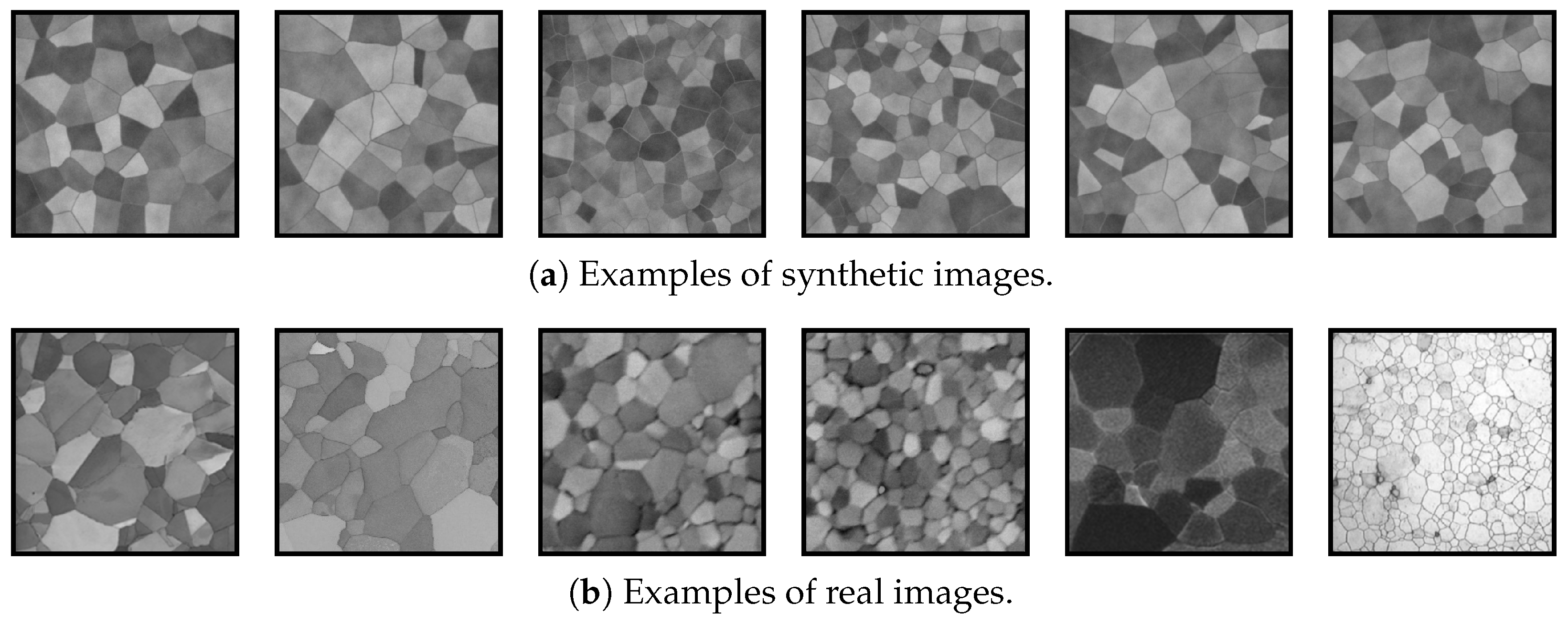
3.2. Grain Boundary Segmentation

Understanding how mechanical properties are related to microstructural features is a core task in materials science applications. One class of such features in metallic materials are grains, i.e., regions that have the same crystallographic orientation. Important statistical properties of a material can be directly linked to the characteristics of the grain size and grain shape distribution. Grains with different orientations appear in images as regions with different intensities or grey shades separated by grain boundaries. As preprocessing it is mandatory to segment these grain boundaries, which is typically a manual task. Furthermore, the extraction of surfaces requires sample preparation and also involves scanning via an electron microscope. This makes each sample acquisition and labelling time consuming and expensive. Automating this process is highly desirable. Hence, we generate synthetic grain structures and the corresponding labels, removing the need for manual labelling or expensive experiments.

3.2.1. Synthetic Data Generation for Training

Synthetic images were created based on Voronoi tessellations implemented in the SciPy library [41].

Using centroids of a random point cloud as seeds for a subsequent Voronoi tessellation reduced larger irregularities of the grain shapes. This is a process that, in physical terms, reduces the interface energy of a grain distribution by penalizing high curvature. The statistical properties of the resulting grain size distribution are different from that of experimentally observed data, nevertheless, they are visually similar. Introducing noise and randomness has been done on different levels. First, real grains are never polygons with perfectly straight segments. Therefore, each segment was replaced by a cubic spline with randomly displaced control points in between the start and end point. Second, real grains come in large varieties of different surface ‘textures’. Synthesizing a representative set together with a dictionary based approach as in the first example was not feasible. Therefore, we used a python generator for Perlin noise (Perlin [42]), which is responsible for large wavelength fluctuation with wave lengths of $\frac{1}{5}$ to $\frac{2}{3}$ grain diameters [43].

Third, noise with short wavelength was added in form of white noise. Finally, a convolution with a Gaussian filter of varying kernel sizes was performed. Besides the already mentioned data augmentation techniques we also applied jitter filters as well as stretching and squishing to the synthetically generated images for training.

Contrary to the crack detection example, now it suffices to have ad hoc examples of the task to be solved. Based on very few samples it should pe possible to guess how a data point can look like. A procedure to generate similar looking data points has to be identified, so that additional synthetic samples can be generated.

3.2.2. Training the Model

We only trained a synthetic model based on artificial grain images with a size of $512\times 512$. We generated 4000 images and divided these into 3200 images for training and 800 images for validation. Instead of directly training on the full resolution images, we trained in three steps via progressive resizing. This subsequent resizing was inspired by Karras et al. [44]. Indeed, this technique lead to more stable training and enhanced model performance. First, the images were downsized to $128\times 128$ and the model head was trained for 20 epochs. Second, the original images were resized to $256\times 256$, the weights were initialized with step one, and the model head was trained for 10 epochs. Finally, we set all model parameters trainable, the weights were initialized with step two, and the model was trained for 5 epochs on the original images of size $512\times 512$.

3.2.3. Evaluation of Synthetic Model

As only 12 real images were available, we manually segmented all images and used these as real data test set. We computed the pixel-wise error and the pixel-wise intersection over union both as mean value ± standard deviation as well as corresponding confidence intervals based on 200 model trainings as described above. The synthetic model resulted in an error of $0.099\pm 0.010$ and the $99\%$ confidence interval was $[0.095,0.10]$. The average intersection over union was $0.745\pm 0.015$ and the corresponding $99\%$ confidence interval was $[0.740,0.0.751]$. For visual inspection some example comparisons of images as well as ground truth and predicted segmentations are depicted in Figure 4 for both real and synthetic images.

Based solely on the metrics the results ca not be easily judged. Both error and intersection over union values are comparable to the best results from Long et al. [36], which indicates the usefulness of the synthetic model. Based on visual examination, the segmentation results are meaningful. Grain boundaries were detected reliably in all real images. The synthetic model had most problems with the width of boundaries, which decreased the values of applied metrics. However, as material scientists are more interested in statistical measures, e.g., number of grains or grain size distribution, than in the correct boundary width, the synthetic model facilitates the analysis in such scenarios. Even for non optimal results, using the predicted segmentation masks as initialization for a further processing ensures a reduced workload and hence a higher throughput when investigating such data.

Unfortunately, it was not possible to train a model solely on actual data, as the provided real images did not suffice to train a meaningful model. Nevertheless, it was possible to train a model with data based only on ad hoc assumptions how the data looks like.

3.3. Adaptation Data Generation and Fine-Tuning

A key benefit of generating synthetic data from parametric models is the possibility to adaptively generate additional data. We demonstrated the principle on the grain boundary example. After each training cycle, we performed inference on the synthetic validation sets. The worst results with respect to the metric were then used as starting point for generating new synthetic data. For each rendered data point, the values of the generating parameters were stored. A fixed number of new data points was generated by changing the stored parameter values within a fixed interval around selected value. We generated additional images with adjusted grain color and boundary thickness, as boundary width and too similar colors of adjacent grains caused the most errors after the first training cycle. We performed a fine-tuning of the models by (i) using additional 1000 random images, and (ii) adaptively generating new training images.

The synthetic validation set contained 1000 images. We selected the $10\%$ of the data points that resulted in the worst intersection over union (IOU). We generated 10 variations of each image for adaptive fine-tuning, such that the total set contained 1000 additional images. The evaluation on the real test set was based on 50 independent training runs.

The error improved from $0.088\pm 0.005$ for the randomly selected data to $0.077\pm 0.003$ for the adaptively sampled data. The IOU improved from $0.763\pm 0.009$ for the random data to $0.778\pm 0.006$. The results are displayed in

Table 2. Evaluation of the adaptive data generation and finetuning procedure. $\mu \pm \sigma$ = mean error ± standard deviation, CI = $99\%$ confidence interval.

		Error	IOU
random data	$\mu \pm \sigma$	$0.088\pm 0.005$	$0.763\pm 0.009$
	CI	$[0.073,0.103]$	$[0.741,0.785]$
adaptive sampling	$\mu \pm \sigma$	$0.077\pm 0.003$	$0.778\pm 0.006$
	CI	$[0.064,0.091]$	$[0.756,0.799]$

. A paired two-tailed t-test showed that the model performance of the adaptive finetuning compared to random finetuning was significantly higher with p-values of $8.6\times {10}^{-18}$ for error and $2.32\times {10}^{-13}$ for IOU. This comparison shows that adaptively generating additional images based on the worst inference results of the former training cycle improves model performance more significantly than adding additional random data points.

4. Discussion

We have presented a workflow to generate synthetic data for training neural networks. The basis of our approach are parametric models that must be available in advance. It is possible to constitute such a model on statistical measurements, known physical constraints, or even simulating the appearance of possible data points. This procedure was implemented and shown based on real world examples with restricted data availability.

The results demonstrated a significant impact of the incorporation of parametrically modelled synthetic data. Models pretrained on the synthetic data outperformed the corresponding real models, or the synthetic models provided useful results for corresponding applications on their own. Based on manually annotated real data the evaluation revealed high benefits for situations where data availability is a problem. Obviously, it must be possible to model the data needed to solve a problem, otherwise the presented approach is not applicable.

A drawback may be the ad hoc character of the approach. Each new problem needs a model generation process before being able to generate synthetic data and train the model. However, there might be many cases where parametric models are already known that must only be integrated into the pipeline. Furthermore, imitating the visual impression of some real examples might not be as time-consuming and tedious as the data acquisition process and related expenses. Furthermore, in many cases in the field of materials science there exists already a simplified, phenomenological simulation model, which might not include all relevant physical details to be a predictive simulation, but which, in the context of a parametric model for synthetic data creation, might be extremely useful. Hence, the proposed procedure may be taken into consideration in each scenario that can be mapped to a parametric model.

5. Conclusions

Summarizing, the presented approach facilitates the training of neural networks by generating artificial data that resemble the reality by employing parametric models. Such models offer the ability to sample data from a parameter space, which may extend the options of regular data acquisition. Hence, synthetic data can be a solution to the fact that in many cases we simply do not have enough data for training—as is often the case in the context of microscopy image data. The variability of training data could be enlarged by a more systematic sampling approach, which will be the focus of future research to further enhance and automate the synthetic data generation workflow.

References

1. Krizhevsky, A.; Sutskever, I.; Hinton, G.E. Imagenet classification with deep convolutional neural networks. Adv. Neural Inf. Process. Syst. 2012, 25, 1097–1105. [Google Scholar] [CrossRef]
2. He, K.; Zhang, X.; Ren, S.; Sun, J. Deep residual learning for image recognition. In Proceedings of the IEEE Conference on Computer Vision and Pattern Recognition, Las Vegas, NV, USA, 27–30 June 2016; pp. 770–778. [Google Scholar]
3. Ronneberger, O.; Fischer, P.; Brox, T. U-net: Convolutional networks for biomedical image segmentation. In International Conference on Medical Image Computing and Computer-Assisted Intervention; Springer: Berlin/Heidelberg, Germany, 2015; pp. 234–241. [Google Scholar]
4. Deng, J.; Dong, W.; Socher, R.; Li, L.J.; Li, K.; Fei-Fei, L. Imagenet: A large-scale hierarchical image database. In Proceedings of the 2009 IEEE Conference on Computer Vision and Pattern Recognition, Miami, FL, USA, 20–25 June 2009; pp. 248–255. [Google Scholar]
5. Yosinski, J.; Clune, J.; Bengio, Y.; Lipson, H. How transferable are features in deep neural networks? In Proceedings of the Advances in Neural Information Processing Systems, Montreal, QC, Canada, 8–13 December 2014; pp. 3320–3328. [Google Scholar]
6. Shin, H.C.; Roth, H.R.; Gao, M.; Lu, L.; Xu, Z.; Nogues, I.; Yao, J.; Mollura, D.; Summers, R.M. Deep convolutional neural networks for computer-aided detection: CNN architectures, dataset characteristics and transfer learning. IEEE Trans. Med Imaging 2016, 35, 1285–1298. [Google Scholar] [CrossRef] [Green Version]
7. Roberts, G.; Haile, S.Y.; Sainju, R.; Edwards, D.J.; Hutchinson, B.; Zhu, Y. Deep Learning for Semantic Segmentation of Defects in Advanced STEM Images of Steels. Sci. Rep. 2019, 9. [Google Scholar] [CrossRef] [Green Version]
8. Masubuchi, S.; Watanabe, E.; Seo, Y.; Okazaki, S.; Sasagawa, T.; Watanabe, K.; Taniguchi, T.; Machida, T. Deep-learning-based image segmentation integrated with optical microscopy for automatically searching for two-dimensional materials. NPJ 2D Mater. App. 2020, 4. [Google Scholar] [CrossRef]
9. Dong, X.; Li, H.; Jiang, Z.; Grünleitner, T.; Güler, I.; Dong, J.; Wang, K.; Köhler, M.H.; Jakobi, M.; Menze, B.H.; et al. 3D Deep Learning Enables Accurate Layer Mapping of 2D Materials. ACS Nano 2021. [Google Scholar] [CrossRef]
10. Furat, O.; Wang, M.; Neumann, M.; Petrich, L.; Weber, M.; Krill, C.E.; Schmidt, V. Machine Learning Techniques for the Segmentation of Tomographic Image Data of Functional Materials. Front. Mater. 2019, 6, 145. [Google Scholar] [CrossRef]
11. Kusche, C.; Reclik, T.; Freund, M.; Al-Samman, T.; Kerzel, U.; Korte-Kerzel, S. Large-area, high-resolution characterisation and classification of damage mechanisms in dual-phase steel using deep learning. PLoS ONE 2019, 14, 1–22. [Google Scholar] [CrossRef] [PubMed] [Green Version]
12. Cordts, M.; Omran, M.; Ramos, S.; Rehfeld, T.; Enzweiler, M.; Benenson, R.; Franke, U.; Roth, S.; Schiele, B. The cityscapes dataset for semantic urban scene understanding. In Proceedings of the IEEE Conference on Computer Vision and Pattern Recognition, Las Vegas, NV, USA, 27–30 June 2016; pp. 3213–3223. [Google Scholar]
13. Russell, B.C.; Torralba, A.; Murphy, K.P.; Freeman, W.T. LabelMe: A database and web-based tool for image annotation. Int. J. Comput. Vis. 2008, 77, 157–173. [Google Scholar] [CrossRef]
14. Acuna, D.; Ling, H.; Kar, A.; Fidler, S. Efficient interactive annotation of segmentation datasets with polygon-rnn++. In Proceedings of the IEEE Conference on Computer Vision and Pattern Recognition, Salt Lake City, UT, USA, 18–23 June 2018; pp. 859–868. [Google Scholar]
15. Xie, J.; Kiefel, M.; Sun, M.T.; Geiger, A. Semantic instance annotation of street scenes by 3d to 2d label transfer. In Proceedings of the IEEE Conference on Computer Vision and Pattern Recognition, Las Vegas, NV, USA, 27–30 June 2016; pp. 3688–3697. [Google Scholar]
16. Srivastava, N.; Hinton, G.; Krizhevsky, A.; Sutskever, I.; Salakhutdinov, R. Dropout: A simple way to prevent neural networks from overfitting. J. Mach. Learn. Res. 2014, 15, 1929–1958. [Google Scholar]
17. Ioffe, S.; Szegedy, C. Batch Normalization: Accelerating Deep Network Training by Reducing Internal Covariate Shift. In Proceedings of the International Conference on Machine Learning, Lille, France, 6–11 July 2015; pp. 448–456. [Google Scholar]
18. Santurkar, S.; Tsipras, D.; Ilyas, A.; Madry, A. How does batch normalization help optimization? arXiv 2018, arXiv:1805.11604. [Google Scholar]
19. Krogh, A.; Hertz, J.A. A simple weight decay can improve generalization. Adv. Neural Inf. Process. Syst. 1995, 4, 950–957. [Google Scholar]
20. Wong, S.C.; Gatt, A.; Stamatescu, V.; McDonnell, M.D. Understanding data augmentation for classification: When to warp? In Proceedings of the 2016 IEEE International Conference on Digital Image Computing: Techniques and Applications (DICTA), Gold Coast, QLD, Australia, 30 November–2 December 2016; pp. 1–6. [Google Scholar]
21. Xu, Y.; Jia, R.; Mou, L.; Li, G.; Chen, Y.; Lu, Y.; Jin, Z. Improved relation classification by deep recurrent neural networks with data augmentation. In Proceedings of the COLING 2016, the 26th International Conference on Computational Linguistics: Technical Papers, Osaka, Japan, 11–16 December 2016; pp. 1461–1470. [Google Scholar]
22. Vasconcelos, C.N.; Vasconcelos, B.N. Increasing deep learning melanoma classification by classical and expert knowledge based image transforms. CoRR abs/1702.07025 2017, 1. [Google Scholar]
23. Richter, S.R.; Vineet, V.; Roth, S.; Koltun, V. Playing for data: Ground truth from computer games. In European Conference on Computer Vision; Springer: Berlin/Heidelberg, Germany, 2016; pp. 102–118. [Google Scholar]
24. Goodfellow, I.; Pouget-Abadie, J.; Mirza, M.; Xu, B.; Warde-Farley, D.; Ozair, S.; Courville, A.; Bengio, Y. Generative adversarial nets. In Proceedings of the Advances in Neural Information Processing Systems, Montreal, QC, Canada, 8–13 December 2014; pp. 2672–2680. [Google Scholar]
25. Karras, T.; Laine, S.; Aila, T. A style-based generator architecture for generative adversarial networks. arXiv 2018, arXiv:1812.04948. [Google Scholar]
26. Shao, S.; Wang, P.; Yan, R. Generative adversarial networks for data augmentation in machine fault diagnosis. Comput. Ind. 2019, 106, 85–93. [Google Scholar] [CrossRef]
27. Poibrenski, A.; Sprenger, J.; Müller, C. Toward a Methodology for Training with Synthetic Data on the Example of Pedestrian Detection in a Frame-by-Frame Semantic Segmentation Task. In Proceedings of the 2018 IEEE/ACM 1st International Workshop on Software Engineering for AI in Autonomous Systems (SEFAIAS), Gothenburg, Sweden, 28 May 2018; pp. 31–34. [Google Scholar]
28. Tremblay, J.; Prakash, A.; Acuna, D.; Brophy, M.; Jampani, V.; Anil, C.; To, T.; Cameracci, E.; Boochoon, S.; Birchfield, S. Training deep networks with synthetic data: Bridging the reality gap by domain randomization. In Proceedings of the IEEE Conference on Computer Vision and Pattern Recognition Workshops, Salt Lake City, UT, USA, 18–22 June 2018; pp. 969–977. [Google Scholar]
29. Wang, M.; Deng, W. Deep visual domain adaptation: A survey. Neurocomputing 2018, 312, 135–153. [Google Scholar] [CrossRef] [Green Version]
30. Sun, B.; Saenko, K. Deep coral: Correlation alignment for deep domain adaptation. In European Conference on Computer Vision; Springer: Berlin/Heidelberg, Germany, 2016; pp. 443–450. [Google Scholar]
31. Dahmen, T.; Trampert, P.; Boughorbel, F.; Sprenger, J.; Klusch, M.; Fischer, K.; Kübel, C.; Slusallek, P. Digital reality: A model-based approach to supervised learning from synthetic data. AI Perspect. 2019, 1, 2. [Google Scholar] [CrossRef] [Green Version]
32. Su, H.; Qi, C.R.; Li, Y.; Guibas, L.J. Render for cnn: Viewpoint estimation in images using cnns trained with rendered 3d model views. In Proceedings of the IEEE International Conference on Computer Vision, Santiago, Chile, 7–13 December 2015; pp. 2686–2694. [Google Scholar]
33. Howard, J.; Gugger, S. Fastai: A Layered API for Deep Learning. Information 2020, 11, 108. [Google Scholar] [CrossRef] [Green Version]
34. Smith, L.N. Cyclical Learning Rates for Training Neural Networks. In Proceedings of the 2017 IEEE Winter Conference on Applications of Computer Vision (WACV), Santa Rosa, CA, USA, 24–31 March 2017; pp. 464–472. [Google Scholar]
35. Agresti, A.; Coull, B.A. Approximate is better than “exact” for interval estimation of binomial proportions. Am. Stat. 1998, 52, 119–126. [Google Scholar]
36. Long, J.; Shelhamer, E.; Darrell, T. Fully convolutional networks for semantic segmentation. In Proceedings of the IEEE Conference on Computer Vision and Pattern Recognition, Boston, MA, USA, 7–12 June 2015; pp. 3431–3440. [Google Scholar]
37. Zabell, S.L. On Student’s 1908 Article “The Probable Error of a Mean”. J. Am. Stat. Assoc. 2008, 103, 1–7. [Google Scholar] [CrossRef]
38. Criminisi, A.; Pérez, P.; Toyama, K. Region filling and object removal by exemplar-based image inpainting. IEEE Trans. Image Process. 2004, 13, 1200–1212. [Google Scholar] [CrossRef]
39. Trampert, P.; Schlabach, S.; Dahmen, T.; Slusallek, P. Exemplar-Based Inpainting Based on Dictionary Learning for Sparse Scanning Electron Microscopy. Microsc. Microanal. 2018, 24, 700–701. [Google Scholar] [CrossRef] [Green Version]
40. Smith, S.L.; Kindermans, P.; Ying, C.; Le, Q.V. Do not Decay the Learning Rate, Increase the Batch Size. In Proceedings of the 6th International Conference on Learning Representations, ICLR 2018, Conference Track Proceedings, Vancouver, BC, Canada, 30 April–3 May 2018; pp. 1–11. [Google Scholar]
41. Virtanen, P.; Gommers, R.; Oliphant, T.E.; Haberland, M.; Reddy, T.; Cournapeau, D.; Burovski, E.; Peterson, P.; Weckesser, W.; Bright, J.; et al. SciPy 1.0: Fundamental Algorithms for Scientific Computing in Python. Nat. Methods 2020, 17, 261–272. [Google Scholar] [CrossRef] [PubMed] [Green Version]
42. Perlin, K. An image synthesizer. ACM Siggraph Comput. Graph. 1985, 19, 287–296. [Google Scholar] [CrossRef]
43. Casey, D. Native-Code and Shader Implementations of Perlin Noise for Python. Available online: https://github.com/caseman/noise (accessed on 3 October 2020).
44. Karras, T.; Aila, T.; Laine, S.; Lehtinen, J. Progressive Growing of GANs for Improved Quality, Stability, and Variation. In Proceedings of the International Conference on Learning Representations, Vancouver, BC, Canada, 30 April–3 May 2018; pp. 1–26. [Google Scholar]
45. Micrograph 712 by DoITPoMS is Licensed under CC-BY-NC-SA Licence. Available online: https://www.doitpoms.ac.uk/miclib/full_record.php?id=712 (accessed on 5 March 2020).
46. TESCAN. Available online: https://www.tescan.com (accessed on 5 March 2020).
47. Rheinheimer, W.; Bäurer, M.; Handwerker, C.A.; Blendell, J.E.; Hoffmann, M.J. Growth of single crystalline seeds into polycrystalline strontium titanate: Anisotropy of the mobility, intrinsic drag effects and kinetic shape of grain boundaries. Acta Mater. 2015, 95, 111–123. [Google Scholar] [CrossRef]
48. Bhattacharyya, J.; Agnew, S.; Muralidharan, G. Texture enhancement during grain growth of magnesium alloy AZ31B. Acta Mater. 2015, 86, 80–94. [Google Scholar] [CrossRef] [Green Version]
Figure 1. Workflow for synthetic data generation. The process starts by creating partial models of reality by modelling or capturing individual aspects such as geometry or physical properties. The partial models are composed of parametric scenarios by manual configuration or data fitting. The composition is performed in such a way that all aspects of reality relevant to a specific simulation are provided. Setting all parameters to fixed values creates a simulation-ready concrete instance of the scenario. This can be used to generate synthetic data, e.g., images, which are used to train a machine learning system. This cycle is then refined iteratively by adapting parts of the pipeline with help of validation processes to enhance the parametric models and the quality of synthetically generated data. Figure adapted from [31].
Crystals 11 00258 g001
Figure 2. ResNet50 architecture. The architecture consists of several sequential blocks: an initial pre-processing block, four sequential blocks each consisting of a downsampling and two ResNet typical residual blocks, and a fully connected output layer. Convolution kernel sizes and number of output channels are provided. Furthermore, stride is taken as one where not shown differently.
Crystals 11 00258 g002
Figure 3. (af) Crack image generation.
Crystals 11 00258 g003
Figure 4. (af) Grain boundary segmentation. Images in (b) from left to right were taken with permission from [45,46], courtesy of Prof. D. Rafaja, TU Bergakademie Freiberg (2 images) [47,48].
Crystals 11 00258 g004aCrystals 11 00258 g004b