An Analytical Study of Internal Heating and Chemical Reaction Effects on MHD Flow of Nanofluid with Convective Conditions

Abstract

This research investigates the influence of the combined effect of the chemically reactive and thermal radiation on electrically conductive stagnation point flow of nanofluid flow in the presence of a stationary magnetic field. Furthermore, the effect of Newtonian heating, thermal dissipation, and activation energy are considered. The boundary layer theory developed the constitutive partial differential momentum, energy, and diffusion balance equations. The fundamental flow model is changed to a system of coupled ordinary differential equations (ODEs) via proper transformations. These nonlinear-coupled equations are addressed analytically by implementing an efficient analytical method, in which a Mathematica 11.0 programming code is developed for numerical simulation. For optimizing system accuracy, stability and convergence analyses are carried out. The consequences of dimensionless parameters on flow fields are investigated to gain insight into the physical parameters. The result of these physical constraints on momentum and thermal boundary layers, along with concentration profiles, are discussed and demonstrated via plotted graphs. The computational outcomes of skin friction coefficient, mass, and heat transfer rate under the influence of appropriate parameters are demonstrated graphically.

1. Introduction

The synthetic industry, oil and gas, atomic energy, electrical energy, etc. are the arenas for the application popular heat transfer phenomena nowadays. The section of particles from various temperatures is viewed as the exchange of heat. Taking everything into account, heat transfer is the progression of heat beyond an object’s limit because of the difference in temperature between the framework and its surrounding environment. The heat transfer in the framework can likewise be performed at various focuses inside the framework as a result of temperature contrasts. The presence of nanoparticles in the liquid furthermore impacts the heat transfer of the liquid. The mixture of solid nanoparticles with a base liquid is known as nanofluid, which was proposed by Choi [1]. There are several groups for the nanoparticles—namely, chemically stable metals (gold, copper), metal oxide (alumina, silica), metal carbides (silicon carbide), metal nitrides (aluminum nitride, silicon nitride), and carbon in various forms (diamond, graphite) [2].

Das et al. [2] numerically enhanced the thermal conductivity of CuO nanofluids channel flow. When nanofluid is utilized instead of traditional fluids, the heat transfer rate increases by 23 percent, according to the study. Juosh [3] reported a dual solution of the MHD viscoelastic nanofluid’s stagnation point on a porous surface with radiation impact. An increment in the Deborah number was found to contribute to a rise in the drag force coefficient. Rashid et al. [4] addressed the MHD stagnation point in a nanofluid flow with a nonuniform thermal reservoir. Pal [5] discussed hydromagnetic stagnation point flow with suction effect, claiming that the Sherwood number diminished as the Lewis number improved. Bioconvective stagnation point Maxwellian nanofluid flow by a convectively heated extended sheet was examined by Abbasi et al. [6]. Lund et al. [7] conducted a stability analysis and discovered a dual solution of magnetohydrodynamic stagnation point Casson fluid flow. Sheikholeslami et al. [8] considered the entropy generation and thermal behavior of nanomaterials using a novel tape solar collector, indicating that energy losses can be decreased by employing nanofluids and twisted tapes. Furthermore, as stated in the study of [9,10,11,12,13,14,15,16,17], and other research studies therein, nanofluids have a variety of features. Due to their importance in applied science and industry, non-Newtonian fluids have recently gained considerable attention. The polymer liquid, animal blood, paint, and detergents are just a few examples of biological fluids. With regard to an MHD flow of Walter-B nanofluid, and studying the viscoelastic nanofluid flow over a permeable cylindrical surface, Hayat et al. [18] examined the effects of mixed convection, heat generation/absorption, and temperature-dependent thermal conductivity. Ramesh and Gireesha [19] explained the effects of heat source/sink characteristics and convective conditions on stretched Maxwell nanofluid flow. In the 3D flow of Burgers nanofluid, Khan et al. [20] evaluated the simultaneous features of heat generation/absorption, thermal radiation, and convective conditions. The impact of viscous dissipation on the 3D-stretched MHD flow of viscous nanoliquid was studied by Mahanthesh et al. [21]. In their analysis, they devised numerical solutions. Hayat et al. [22,23,24] used stretching surface flows of thixotropic, Burgers, and viscoelastic fluids. The Arrhenius activation energy is one of the important criteria that is often overlooked while studying species chemical reactions. Arrhenius was the first to discover activation energy [25]. He asserted that only a minimal amount of energy is required to start a chemical reaction between atoms and molecules. Magnetohydrodynamics has been extensively used to solve problems in science and technology, as well as on a large industrial scale, and the demand continues to grow. Petroleum and metallurgical operations are two examples [26]. The quality of the products in such instances is determined by the rate of cooling. Many researchers have considered it in their research since its inception, to investigate its impact on fluid characteristics. Numerous studies have recently been published in which MHD has a major impact. Hsiao [27] examined the electrical magnetohydrodynamic Maxwell nanofluid with radiation and viscous dissipation effects, for example. The dynamics of a hydromagnetic cross nanofluid in the presence of gyrotactic microorganisms was the subject of a study by Naz et al. [28]. Atif et al. [29] investigated the magnetic properties of tangent hyperbolic nanofluid passing via a stretching wedge in another investigation. Animal blood, polymer liquid, paint, food, and detergents are some examples of biological fluids. With regard to the MHD flow of Walter-B nanofluid, Qayyum et al. [30] investigated the chemical reaction impacts. These citations [31,32,33,34] provide more studies on activation energy. In what follows, specific objectives of this analytical study that have not been considered thus far are elucidated, and they include the following:

(1)

To explore time subservient Walter-B nanofluid flow resulting from the impression of heat and mass transfer and thermal radiation/absorption, along with chemical reaction;

(2)

Mathematical modeling of the fundamental flow equations that comprises momentum, energy, and diffusion balances;

(3)

To impose an analytical method for attaining the upshots. Additionally, to reduce a stability and convergence study for optimizing flow constraints;

(4)

To display the impact of diversified pertinent parameters on flow fields, together with skin friction force, heat transfer, and mass transfer profiles;

(5)

To show the advanced 3D form of the fluid flow.

2. Mathematical Modeling

We considered these effects on the magnetohydrodynamic flow over a stretching surface. Figure 1 shows the flow configuration of two-dimensional Walters-B nanofluid flow due to stretching surface under the influence of the stationary magnetic field. The influence of heat transfer, Brownian and thermophoretic effects were considered. Furthermore, the heat flow mechanism was evaluated by assuming the thermal radiation, Joule heating, and viscous dissipation, and heat generation/absorption characteristics were taken into consideration. The fluid was electrically conductive, along with a uniform magnetic field $B_0$ in the normal direction. Based on these assumptions, with regard to the approximations of the boundary layer, the basic equations of reduced incompressible Walter-B nanofluid are as follows [30]:

$$\frac{\partial u^{*}}{\partial x^{*}}+\frac{\partial v^{*}}{\partial y^{*}}=0$$

(1)

$$\begin{array}{l}{u}^{*}\frac{\partial u^{*}}{\partial x^{*}}+v^{*}\frac{\partial u^{*}}{\partial y^{*}}=u_e\frac{\partial u_e}{\partial x^{*}}+\nu \frac{\partial u^{*2}}{\partial y^{*2}}-\frac{k_0}{{\rho }_f}\left(u^{*}\frac{{\partial }^3{u}^{*}}{\partial x^{*}\partial y^{*2}}+v^{*}\frac{{\partial }^3{u}^{*}}{\partial y^{*3}}+\frac{\partial u^{*}}{\partial x^{*}}\frac{{\partial }^2{u}^{*}}{\partial y^{*2}}-\frac{\partial u^{*}}{\partial y^{*}}\frac{{\partial }^2{u}^{*}}{\partial x^{*}\partial y^{*}}\right)\\ +\frac{\sigma B_0^2}{{\rho }_f}\left(u_e-u^{*}\right)+g{\beta }_T\left(T-T_{\infty }\right)-g{\beta }_C\left(C-C_{\infty }\right)\end{array}$$

(2)

$$\begin{array}{l}{u}^{*}\frac{\partial T^{*}}{\partial x^{*}}+v^{*}\frac{\partial T^{*}}{\partial y^{*}}=\alpha \left(\frac{{\partial }^2{T}^{*}}{\partial y^{*2}}\right)-\frac{1}{{\left(\rho c\right)}_f}\frac{16{\sigma }^{*}}{3k^{*}}\frac{\partial }{\partial y^{*}}\left(T^{*3}\frac{\partial T^{*}}{\partial y^{*}}\right)+\frac{\sigma B_0^2{u}^{*2}}{{\left(\rho c\right)}_f}+\\ \tau \left(D_B\frac{\partial C^{*}}{\partial y^{*}}\frac{\partial T^{*}}{\partial y^{*}}+\frac{D_T}{T_{\infty }^{*}}{\left(\frac{\partial T^{*}}{\partial y^{*}}\right)}^2\right)+\frac{Q_0}{{\left(\rho c\right)}_f}\left(T^{*}-T_{\infty }^{*}\right)\end{array}$$

(3)

$$u^{*}\frac{\partial C^{*}}{\partial x^{*}}+v^{*}\frac{\partial C^{*}}{\partial y^{*}}=D_B\left(\frac{{\partial }^2{C}^{*}}{\partial y^{*}{}^2}\right)+\frac{D_T}{T_{\infty }^{*}}\left(\frac{{\partial }^2{T}^{*}}{\partial y^{*2}}\right)-k_r^2{e}^{-\frac{E_a}{k{T}^{*}}}{\left(\frac{T^{*}}{T_{\infty }^{*}}\right)}^m\left(C^{*}-C_{\infty }^{*}\right)$$

(4)

with boundary postulates

$$\begin{array}{l}{u}^{*}=u_w\left(x^{*}\right)=c_1{x}^{*}, v=0,-k\frac{\partial T^{*}}{\partial y^{*}}=\left(T_s^{*}-T^{*}\right)h_1,-D_B\frac{\partial C^{*}}{\partial y^{*}}=\left(C_s^{*}-C^{*}\right)h_2 at y^{*}=0\\ u^{*}=u_e=c_2{x}^{*} , T^{*}\to T_{\infty }^{*}, C^{*}\to C_{\infty }^{*} at y^{*}\to \infty \end{array}$$

(5)

where $\left(u^{*},v^{*}\right)$ is the velocity component in $x^{*}\text{-}$ and $y^{*}\text{-}\mathrm{d}\mathrm{i}\mathrm{r}\mathrm{e}\mathrm{c}\mathrm{t}\mathrm{i}\mathrm{o}\mathrm{n}$; $u_e$ is the free stream velocity; $D_B$ is the Brownian motion; $D_T$ is the thermophoretic coefficient; $g$ is the gravitational acceleration; $C^{*}$ is the fluid concentration; $T^{*}$ is the temperature; $\alpha ={k/\rho c}_f$ is thermal diffusion coefficient; $\nu ={{\mu }_0/\rho }_f$ is the kinematic viscosity; ${\sigma }^{*}$ is the Stefan–Boltzman constant; $k^{*}$ is the absorption coefficient; ${\beta }_{C^{*}}$ denotes the solutal expansion coefficient; ${\beta }_{T^{*}}$ is the thermal expansion coefficient; $\tau$ is the heat capacity ratio; $\sigma$ is electrical conductivity; $Q_0$ is heat generation/absorption; $Ea$ is the activation energy; $T_s^{*}$ is the surface temperature; $C_s^{*}$ is the surface concentration; $h_1$ is the heat transfer coefficient; $h_2$ is the mass transfer coefficient; $m$ is the fitted rate constant; $kr$ is the reaction rate; $T_{\infty }^{*}$ is the ambient temperature, $C_{\infty }^{*}$ is the ambient concentration; $k_0$ is the short memory coefficient.

A set of similarity transformations that lead to non-dimensionalities of the governing equations is given by

$$u^{*}=c_1{x}^{*}{f}^{\prime }\left(\xi \right), v^{*}=-{\left(c_1\nu \right)}^{\frac{1}{2}}f\left(\xi \right), \xi =\sqrt{\frac{c_1}{\nu }}{y}^{*}, T=\frac{T^{*}-T_{\infty }^{*}}{T_s^{*}-T_{\infty }^{*}}, C=\frac{C^{*}-C_{\infty }^{*}}{C_s^{*}-C_{\infty }^{*}}$$

(6)

By utilizing these transformation variables, Equation (1) is commonly valid, whereas Equations (2)–(5) diminish to

$$f^{‴}-{f^{\prime }}^2+f{f}^{″}+We\left({f^{″}}^2-2f^{\prime }{f}^{‴}+f{f}^{⁗}\right)+M\left(A-f^{\prime }\right)+A^2+\lambda \left(T+NC\right)=0$$

(7)

$${\left(\left(1+\frac{3}{4}R{\left(1+\left(T_f-1\right)T\right)}^3\right)T^{\prime }\right)}^{\prime }+\mathrm{Pr}\left(f{T}^{\prime }+Nb{T}^{\prime }{C}^{\prime }+Nt{\left(T^{\prime }\right)}^2+MEc{\left(f^{\prime }\right)}^2+ST\right)=0$$

(8)

$$C^{″}+Scf{C}^{\prime }+\left(\frac{Nt}{Nb}\right)T^{″}-Sc\sigma {\left(1+{\delta }_{1}T\right)}^{m}C\exp \left[\frac{-E_1}{1+{\delta }_{1}T}\right]=0$$

(9)

$$\begin{array}{l}f\left(0\right)=0, f^{\prime }\left(0\right)=1, T^{\prime }\left(0\right)=-\alpha \left(1-T\left(0\right)\right), C^{\prime }\left(0\right)=-\beta \left(1-C\left(0\right)\right) \\ f^{\prime }(\infty )=A, T(\infty )=0, C(\infty )=0 \end{array}$$

(10)

$$\begin{array}{l}M=\frac{\sigma B_0^2}{{\rho }_f{c}_1};We=\frac{k_0{c}_1}{{\mu }_0};\lambda =\frac{g{\beta }_{\overline{T}}}{c_1^2{x}^{*}}\left(T_s^{*}-T_{\infty }^{*}\right);N=\frac{g{\beta }_{\overline{C}}}{c_1^2{x}^{*}}\left(C_s^{*}-C_{\infty }^{*}\right);Nt=\frac{\tau D_T}{T_{\infty }^{*}\nu }\left(T_s^{*}-T_{\infty }^{*}\right);\\ Nb=\frac{\tau D_B}{\nu }\left(C_s^{*}-C_{\infty }^{*}\right);{\delta }_1=\frac{T_s^{*}-T_{\infty }^{*}}{T_{\infty }^{*}};R=\frac{4{\sigma }^{*}{T}_{\infty }^{*3}}{k{k}^{*}};S=\frac{Q_0}{{\left(\rho c\right)}_f{c}_1};Ec=\frac{u_w^{*2}}{c_f\left(T_s^{*}-T_{\infty }^{*}\right)};\\ E_1=\frac{E_a}{\kappa T_{\infty }^{*}};{\theta }_f=\frac{T_w^{*}}{T_{\infty }^{*}};A=\frac{c_2}{c_1};\sigma =\frac{k_r^2}{c_1};Sc=\frac{\nu }{D_B};\mathrm{Pr}=\frac{\mu c_p}{k};B_1=\frac{h_1}{k}\sqrt{\frac{\nu }{\gamma }};B_2=\frac{h_2}{D_B}\sqrt{\frac{\nu }{\gamma }};\end{array}$$

Here, the significant physical quantities are labeled as the magnetic parameter; Weissenberg number; mixed convection parameter; the ratio of thermal to concentration buoyancy forces; thermophoresis parameter; Brownian parameter; temperature difference; radiation parameter; heat generation parameter; Eckert number; activation energy; temperature ratio parameter; the ratio of rate constant; dimensionless reaction rate; Schmidt number; Prandtl number; thermal Biot number; solutal Biot number.

3. Quantities of Interest

The important engineering quantities of interest are the surface drag force, temperature gradient, and concentration gradient at surface, defined as follows:

$$C{f}_x=\frac{2{\tau }_w}{\rho u_w^2}$$

(11)

$${\tau }_w={\mu }_0{\left(\frac{\partial u^{*}}{\partial y^{*}}\right)}_{y^{*}=0}-k_0{\left(u^{*}\frac{{\partial }^2{u}^{*}}{\partial x^{*}\partial y^{*}}+2\frac{\partial u^{*}}{\partial x^{*}}\frac{\partial u^{*}}{\partial y^{*}}\right)}_{y^{*}=0}$$

(12)

One can obtain the $C{f}_x$ in non-dimensional form by substituting Equation (12) in Equation (11).

$$\sqrt{{\mathrm{Re}}_x}C{f}_x=1-3B{f}^{\prime }\left(0\right)f^{″}\left(0\right)$$

(13)

$$N{u}_x=\frac{x^{*}{q}_w}{k\left(T_f^{*}-T_{\infty }^{*}\right)}$$

(14)

$$q_w={-k\left(1+\frac{16}{3}\frac{{\sigma }^{*}{T}^{*3}}{k{k}^{*}}\right)\frac{\partial T^{*}}{\partial y^{*}}|}_{y^{*}=0}$$

(15)

Inputting Equation (15) into Equation (14) allows $N{u}_x$ to be obtained in the dimensionless form as follows:

$$\frac{N{u}_x}{\sqrt{{\mathrm{Re}}_x}}=-\left(1+\frac{4}{3}R{\left(1+\left(T_f-1\right)T\left(0\right)\right)}^3\right)T^{\prime }\left(0\right)$$

(16)

$$S{h}_x=\frac{x^{*}{j}_w}{k\left(C_f^{*}-C_{\infty }^{*}\right)}$$

(17)

$$j_w={\frac{\partial C^{*}}{\partial y^{*}}|}_{y^{*}=0}$$

(18)

Similarly, with help of Equations (17) and (18), one obtains $S{h}_x$ in the dimensionless form.

$$\frac{S{h}_x}{\sqrt{{\mathrm{Re}}_x}}=-C^{\prime }\left(0\right)$$

(19)

where $q_w$ is the heat flux; $j_w$ is the mass flux; ${\tau }_w$ is the wall shear stress; ${\mathrm{Re}}_x=c_1{x}^2/\nu$ is the Reynold number.

4. Homotopic Solution (HAM)

To solve Equations (7)–(9), subject to the extreme postulates given in Equation (10), we used the homotopic analysis method. The solution procedures have an auxiliary parameter, $\hslash$, which adjusts and controls the convergence region of the stable solutions. The following are the opted assumptions:

$$f_0(\xi )=1-A+A\xi +(A-1)e^{-\xi }, T_0(\xi )=\frac{\alpha }{1+\alpha }{e}^{-\xi }, C_0(\xi )=\frac{\beta }{1+\beta }{e}^{-\xi },$$

(20)

The linear operators are $L_f,{\mathrm{L}}_T{, \mathrm{L}}_C$,

$$L_f(f)=f^{‴}-f^{\prime },{ \mathrm{L}}_T(T)=T^{″}\hspace{0.17em}-T,{ \mathrm{L}}_C(C)=C^{″}-C$$

(21)

with the following properties:

$$L_f(c_1+c_2{e}^{-\xi }+c_3{e}^{\xi })=0,{ \mathrm{L}}_T(c_4{e}^{\xi }+c_5{e}^{-\xi })=0,{ \mathrm{L}}_C(c_6{e}^{\xi }+c_7{e}^{-\xi })=0,$$

(22)

where $c_i(i=1-7)$ are the constants.

The non-linear operatives $N_f,N_g,N_T{, N}_C$ are

$$\begin{array}{l}{N}_f\left[f(\xi ;p),T(\xi ;p),C(\xi ;p)\right]=\frac{{\partial }^{3}f(\xi ;p)}{\partial {\xi }^3}-{\left(\frac{\partial f(\xi ;p)}{\partial \xi }\right)}^2+f(\xi ;p)\frac{{\partial }^{2}f(\xi ;p)}{\partial {\xi }^2}+\\ +B\left({\left(\frac{{\partial }^{2}f(\xi ;p)}{\partial {\xi }^2}\right)}^2-2\frac{\partial f(\xi ;p)}{\partial \xi }\frac{{\partial }^{3}f(\xi ;p)}{\partial {\xi }^3}+f(\xi ;p)\frac{{\partial }^{4}f(\xi ;p)}{\partial {\xi }^4}\right)+M\left(A-\frac{\partial f(\xi ;p)}{\partial \xi }\right)\\ +A^2+\lambda \left(T(\xi ;p)+NC(\xi ;p)\right)\end{array}$$

(23)

$$\begin{array}{l}{N}_T\left[f(\xi ;p),T(\xi ;p),C(\xi ;p),\right]={\left(\left(1+\frac{4}{3}R\left(1+{\left({\theta }_f-1\right)}^3\right)\frac{\partial T(\xi ;p)}{\partial \xi }\right)\right)}^{\prime }+\\ \mathrm{Pr}\left[\begin{array}{l}f(\xi ;p)\frac{\partial T(\xi ;p)}{\partial \eta }+Nb\frac{\partial T(\xi ;p)}{\partial \xi }\frac{\partial C(\xi ;p)}{\partial \xi }+Nt{\left(\frac{\partial T(\xi ;p)}{\partial \xi }\right)}^2+\\ ME{c}^2{\left(\frac{\partial f(\xi ;p)}{\partial \xi }\right)}^2+\delta T(\xi ;p)\end{array}\right]\end{array}$$

(24)

$$\begin{array}{l}{N}_C\left[f(\xi ;p),T(\xi ;p),C(\xi ;p)\right]=\frac{{\partial }^{2}C(\xi ;p)}{\partial {\xi }^2}+Scf(\xi ;p)\frac{\partial C(\xi ;p)}{\partial \xi }+\\ \frac{Nt}{Nb}\frac{{\partial }^{2}T(\xi ;p)}{\partial {\xi }^2}-Sc\sigma {\left(1+{\delta }_{1}T(\xi ;p)\right)}^{m}C(\xi ;p)Exp\left[-\frac{E_1}{1+{\delta }_{1}T(\xi ;p)}\right]\end{array}$$

(25)

The working rules of the homotopic scheme are designated in [35,36,37,38,39], and the 0th-order problems from Equations (7)–(9) are

$$(1-p)L_f\left[f(\xi ;p)-f_0(\xi )\right]=p{\hslash }_f{N}_f\left[f(\xi ;p),T(\xi ;p),C(\xi ;p)\right]$$

(26)

$$(1-p)L_T\left[T(\xi ;p)-T_0(\xi )\right]=p{\hslash }_T{N}_T\left[f(\xi ;p),T(\xi ;p),C(\xi ;p)\right]$$

(27)

$$(1-p)L_C\left[C(\xi ;p)-C_0(\xi )\right]=p{\hslash }_C{N}_C\left[f(\xi ;p),T(\xi ;p),C(\xi ;p)\right]$$

(28)

The equivalent boundary conditions are

$$\begin{array}{l}{f(\xi ;p)|}_{\xi =0}=0, {\frac{\partial f(\xi ;p)}{\partial \xi }|}_{\eta =0}=1, {\frac{\partial f(\xi ;p)}{\partial \xi }|}_{\xi \to \infty }=A,\\ {\frac{\partial T(\xi ;p)}{\partial \xi }|}_{\xi =0}=-\alpha \left({1-T(\xi ;p)|}_{\xi =0}\right), {T(\xi ;p)|}_{\xi \to \infty }=0, \\ {\frac{\partial C(\xi ;p)}{\partial \xi }|}_{\xi =0}=-\beta \left({1-C(\xi ;p)|}_{\eta =0}\right), {C(\xi ;p)|}_{\xi \to \infty }=0\end{array}$$

(29)

where $p\in [0,1]$ is the embedding parameter, and ${\hslash }_f, {\hslash }_T, {\hslash }_C$ are used to control the convergence of the solution. When $p=0 \mathrm{and} p=1$, we have

$$f(\xi ;1)=f(\xi ), T(\xi ;1)=T(\xi ), C(\xi ;1)=C(\xi )$$

(30)

Expanding $f(\xi ;p), T(\xi ;p), C(\xi ;p)$ in Taylor’s series about $p=0$,

$$\begin{array}{l}f(\xi ;p)=f_0(\xi )+{\displaystyle \sum _{m=1}^{\infty }{f}_m(\xi )p^m}, \\ T(\xi ;p)=T_0(\xi )+{\displaystyle \sum _{m=1}^{\infty }{T}_m(\xi )p^m},\\ C(\xi ;p)=C_0(\xi )+{\displaystyle \sum _{m=1}^{\infty }{C}_m(\xi )p^m}.\end{array}$$

(31)

where

$$f_m(\xi )={\frac{1}{m!}\frac{\partial f(\xi ;p)}{\partial \xi }|}_{p=0},T_m(\xi )={\frac{1}{m!}\frac{\partial T(\xi ;p)}{\partial \xi }|}_{p=0}, {\varphi }_m(\xi )={\frac{1}{m!}\frac{\partial C(\xi ;p)}{\partial \xi }|}_{p=0},$$

(32)

The parameters ${\hslash }_f, {\hslash }_T, {\hslash }_C$ are selected in such a way that the series in Equation (31) converges at $p=1$, switching $p=1$ in Equation (27), we obtain

$$\begin{array}{l}f(\xi )=f_0(\xi )+{\displaystyle \sum _{m=1}^{\infty }{f}_m(\xi )},\\ T(\xi )=T_0(\xi )+{\displaystyle \sum _{m=1}^{\infty }{T}_m(\xi )},\\ C(\xi )=C_0(\xi )+{\displaystyle \sum _{m=1}^{\infty }{C}_m(\xi )}.\end{array}$$

(33)

The mth order problem satisfies the following:

$$\begin{array}{l}{L}_f\left[f_m(\xi )-{\chi }_m{f}_{m-1}(\xi )\right]={\hslash }_f{R}_m^f(\xi ),\\ L_T\left[T_m(\xi )-{\chi }_m{T}_{m-1}(\xi )\right]={\hslash }_T{R}_m^T(\xi ),\\ L_C\left[C_m(\xi )-{\chi }_m{C}_{m-1}(\xi )\right]={\hslash }_C{R}_m^C(\xi ).\end{array}$$

(34)

The extremes conditions are

$$\begin{array}{l}{f}_m(0)={f^{\prime }}_m(0)=T_m(0)=C_m(0)=0\\ {f^{\prime }}_m(\infty )=T_m(\infty )=C_m(\infty )=0\end{array}$$

(35)

Here,

$$\begin{array}{l}{R}_m^f(\xi )={f^{‴}}_{m-1}-{\displaystyle \sum _{k=0}^{m-1}{f^{\prime }}_{m-1-k}}{f^{\prime }}_k+{\displaystyle \sum _{k=0}^{m-1}{f}_{m-1-k}}{f^{″}}_k+M\left(A-{f^{\prime }}_{m-1}\right)\\ B\left({\displaystyle \sum _{k=0}^{m-1}{f^{″}}_{m-1-k}}{f^{″}}_k-2{\displaystyle \sum _{k=0}^{m-1}{f^{\prime }}_{m-1-k}}{f^{‴}}_k+{\displaystyle \sum _{k=0}^{m-1}{f}_{m-1-k}}{f^{⁗}}_k\right)+A^2+\lambda \left(T_{m-1}+N{C}_{m-1}\right),\end{array}$$

(36)

$$\begin{array}{l}{R}_m^T(\xi )={\left(1+\frac{4}{3}R\left(1+{\left({\theta }_f-1\right)}^3\right)T_{m-1}^{\prime }\right)}^{\prime }+\\ \mathrm{Pr}\left[{\displaystyle \sum _{k=0}^{m-1}{f}_{m-1-k}}{T}_k^{\prime }+Nb{\displaystyle \sum _{k=0}^{m-1}{T}_{m-1-k}^{\prime }}{C}_k^{\prime }+Nt{\displaystyle \sum _{k=0}^{m-1}{T}_{m-1-k}^{\prime }{T}_k^{\prime }}+ME{c}^2{\displaystyle \sum _{k=0}^{m-1}{f^{\prime }}_{m-1-k}}{f^{\prime }}_k+S{T}_{m-1}\right]\end{array}$$

(37)

$$R_m^C(\xi )={{\varphi }^{″}}_{m-1}+Sc\left[{\displaystyle \sum _{k=0}^{m-1}{f}_{m-1-k}}{C}_k^{\prime }\right]+\frac{Nt}{Nb}{T}_{m-1}^{″}-Sc\sigma {\left(1+{\delta }_1{T}_{m-1}\right)}^m{C}_{m-1}Exp\left[\frac{-E_1}{1+{\delta }_1{C}_{m-1}}\right]$$

(38)

whereas,

$${\chi }_m=\{\begin{array}{l}0, \mathrm{if} \mathrm{p}\le 1\\ 1, \mathrm{if} \mathrm{p}>1\end{array}$$

5. Convergence and Stability Analysis

The series solutions developed by the homotopic analysis method (HAM) comprised the convergence control parameters ${\hslash }_f,{\hslash }_T$, and ${\hslash }_C$. These convergence control parameters were effective at regulating and controlling the convergence area of the series solutions. The $\hslash \text{-}curves$ were studied to the 30th order of approximation. The admissible values were obtained by the flat parts of the $\hslash \text{-}curves$. Figure 1 and Figure 2 display the acceptable ranges of ${\hslash }_f,{\hslash }_T$ and ${\hslash }_C$ are $-1.5\le {\hslash }_f\le -0.5$, $-1.3\le {\hslash }_T\le -0.4$ and $-0.8\le {\hslash }_C\le -0.2$ respectively.

Figure 1. For $f\left(\xi \right)$ and $T\left(\xi \right)$ functions.

Figure 1. For $f\left(\xi \right)$ and $T\left(\xi \right)$ functions.

Moreover,

Table 1. Convergence analysis via distinct order approximations.

Order of Approximations	$-{\mathit{f}}^{″}\left(0\right)$	$-{\mathit{T}}^{\prime }\left(0\right)$	$-{\mathit{C}}^{\prime }\left(0\right)$
1	$-0.999044$	$-0.347683$	$0.303896$
5	$-0.993083$	$-0.315678$	$0.281513$
10	$-0.986753$	$-0.266432$	$0.281513$
15	$-0.980398$	$-0.216247$	$0.281513$
25	$-0.968326$	$-0.216247$	$0.281513$
30	$-0.968326$	$-0.216247$	$0.281513$

discloses convergence analysis computationally. Here, 30th-order approximations are adequate for Equations (7)–(9) convergence.

6. Discussion

In this section, the basic flow nature and fluid properties due to the effects of the relevant physical parameter were considered. Additionally, the impacts of relevant constraints on flow fields such as surface drag force, heat, and mass flow coefficients were analyzed through plotted graphs. The default values of the governing parameters are

$$\begin{array}{c}Rd=0.4;{\theta }_f=0.3;Nb=Nt=0.5;B_1=0.4,B_2=1.0;S=0.5;Ec=0.3;\mathrm{Pr}=1.0;E_1=0.5;Sc=0.4\\ M=0.1;A=0.2;We=0.5;\lambda =0.5;N=1.0\end{array}$$

Figure 3 explains $f^{\prime }\left(\xi \right)$ outlines retarded estimates, with a higher estimation of $M$. From a physical point of view, the apparent fluid viscosity increases when $M$ is introduced to any fluid. As the magnetic field intensity rises, a resistive nature in liquid flow is initiated, known as Lorentz dynamism, which obstructs the flow significantly.

From Figure 4, it can be inferred that the impact of $M$ is to raise the $f^{\prime }\left(\xi \right)$ thermal energy with higher $M$ values. It is observed that as $M$ increases, it exits the nanoparticles, which diffuse rapidly in the neighboring layers. Variations in ratio parameter $A$ for analyzing the $f^{\prime }\left(\xi \right)$ profiles are unveiled in Figure 5. As shown in the figure, an increment in $f^{\prime }\left(\xi \right)$ outlines is evident with higher $A$ estimations. The outcome of $We$ on $f^{\prime }\left(\xi \right)$ profiles is depicted in Figure 6. As anticipated, the flow field diminishes with higher data of $We$ values. In reality, the material relaxation time increases, which causes resistance in fluid flow. Subsequently, $f^{\prime }\left(\xi \right)$ outlines decline. The flow $f^{\prime }\left(\xi \right)$ field for the $\lambda$ is shown in Figure 7. It is observed that the $f^{\prime }\left(\xi \right)$ distribution increases, as the value of $\lambda$ increases, due to the buoyancy factor.

Figure 8 demonstrates the role of the ratio parameter $N$ on $f^{\prime }\left(\xi \right)$. An increase in $N$ corresponds to a rise in the flow field.

Figure 9 uncovers the variations that were realized in the fluid $T\left(\xi \right)$ due to the increment in the values of $Rd$ factor. It can be observed that $T\left(\xi \right)$ rises as radiation develops because of the conduction effect of the nanofluid as a result of thermal radiation. Therefore, increasing $Rd$ implies higher surface heat flux and thus upsurges the $T\left(\xi \right)$ inside the boundary layer region. Attributes of ${\theta }_f$ on thermal field $T\left(\xi \right)$ are revealed in Figure 10. Here, the thermal energy increases via higher estimations of ${\theta }_f$.

Figure 11 reveals the $Nb$ impact on energy fields. As expected, heat transfer increases. In nanofluids, the $Nb$ effect rises due to the nanoparticles, and at this point, the rapid motion of the nanometer-scale molecules and its resulting impact on the fluid contribute significantly to the heat transfer mechanism. An increment in $Nb$ yields effective movement of random nanoparticle molecules inside the liquid. The influence of this irregular motion enhances molecule energy (kinetic force), and ultimately, $T\left(\xi \right)$ increases.

Figure 12 elucidates the influence of the random nanoparticle’s movement represented by $Nb$ on the $C\left(\xi \right)$ outlines. The nanoparticle Brownian motion at the molecular level performs a central role in determining the thermal performance of nanoparticle suspensions. It is obvious that $C\left(\xi \right)$ diminishes with an increase in the $Nb$ parameter.

Figure 13 indicates variations in the energy curves subject to the $Nt$ parameter. Here, $T\left(\xi \right)$ enhances through higher $Nt$. Physically, thermophoretic influence increases, as $Nt$ is augmented. Such force facilitates the escape of small molecules from hotter to colder parts, and eventually, $T\left(\xi \right)$ increases.

Figure 14 explains the $Nt$ impact on $C\left(\xi \right)$ profiles. Here, an increase in $C\left(\xi \right)$ is detected, which is subjected to larger $Nt$ assessments. Physically, an upsurge in thermophoretic force is observed through a higher $Nt$ parameter, which frequently moves molecules from higher- toward lower-temperature regions. Hence, $C\left(\xi \right)$ increases.

Figure 15 describes the $B_1$ effect on thermal field curves. Increasing the data of $B_1$ develops the fluid $T\left(\xi \right)$ profiles, as well as the rate of heat transfer of the nanofluids. From a physical point of view, $B_1$ has the ability to increase the temperature difference between the nanoparticles. This leads to augmenting the $T\left(\xi \right)$ curves.

Figure 16 displays variation in $T\left(\xi \right)$ subject to different values of $S$. It is observed that a rise in $S$ values increases the $T\left(\xi \right)$ field. It is worth noting that larger $S$ values can add extra heat to the nanofluid due to which thermal field upsurges. Variations in $T\left(\xi \right)$ curves through higher estimation of $Ec$ is plotted in Figure 17. Here, the thermal field rises with increasing values of $Ec$. Physically, higher $Ec$ adds more heat to the internal system due to which the nanoparticles have higher kinetic energy releases; consequently, $T\left(\xi \right)$ increases. The role of $\mathrm{Pr}$ on thermal field is evaluated in Figure 18. It is seen that the thermal diffusivity diminishes, subject to higher estimation of $\mathrm{Pr}$ values. In consequence, $T\left(\xi \right)$ decreases.

Figure 19 elucidates the $E_1$ effect on fluid $C\left(\xi \right)$ profiles. As estimated, the $C\left(\xi \right)$ augments through larger activation energy parameter $E_1$.

Figure 20 delineates the $Sc$ effect on fluid concentration. Physically, $Sc$ and $D$ are related inversely. Thus, an upsurge in $Sc$ causes a decline in $C\left(\xi \right)$ curves. From a physical point of view, $D$ declines as $Sc$ increases. Hence, $C\left(\xi \right)$ diminishes. The concentration profiles of $C\left(\xi \right)$ for $B_2$ are unveiled in Figure 21. Clearly, $C\left(\xi \right)$ is an increasing function of $B_2$. The mass transference coefficient $h_2$ increases once $B_2$ is improved. Consequently, $C\left(\xi \right)$ increases. The impact of the drag force coefficient $C{f}_x$ against the different values of $M$ and $A$ is depicted in Figure 22. This figure reveals that $C{f}_x$ is a growing function of both parameters. Attributes of $Nb$ and $Nt$ influences on heat transfer coefficient $N{u}_x$ are shown in Figure 23. This graph confirms that $N{u}_x$ diminishes, subject to enlarged Brownian and thermophoresis parameters. Figure 24 designates the effects of $Nb$ and $Sc$ on mass flow coefficient $S{h}_x$. As it is observed from this plot, $S{h}_x$ increases with larger data of these parameters.

7. Closing Remarks

In this study, we examined the magnetohydrodynamic effect on the 2D stagnation point flow of a viscoelastic Walter-B nanofluid in view of a magnetic field, along with thermal radiation, heat and mass transfer, and convective boundary conditions. The resulting critical remarks are summarized as follows:

(1)

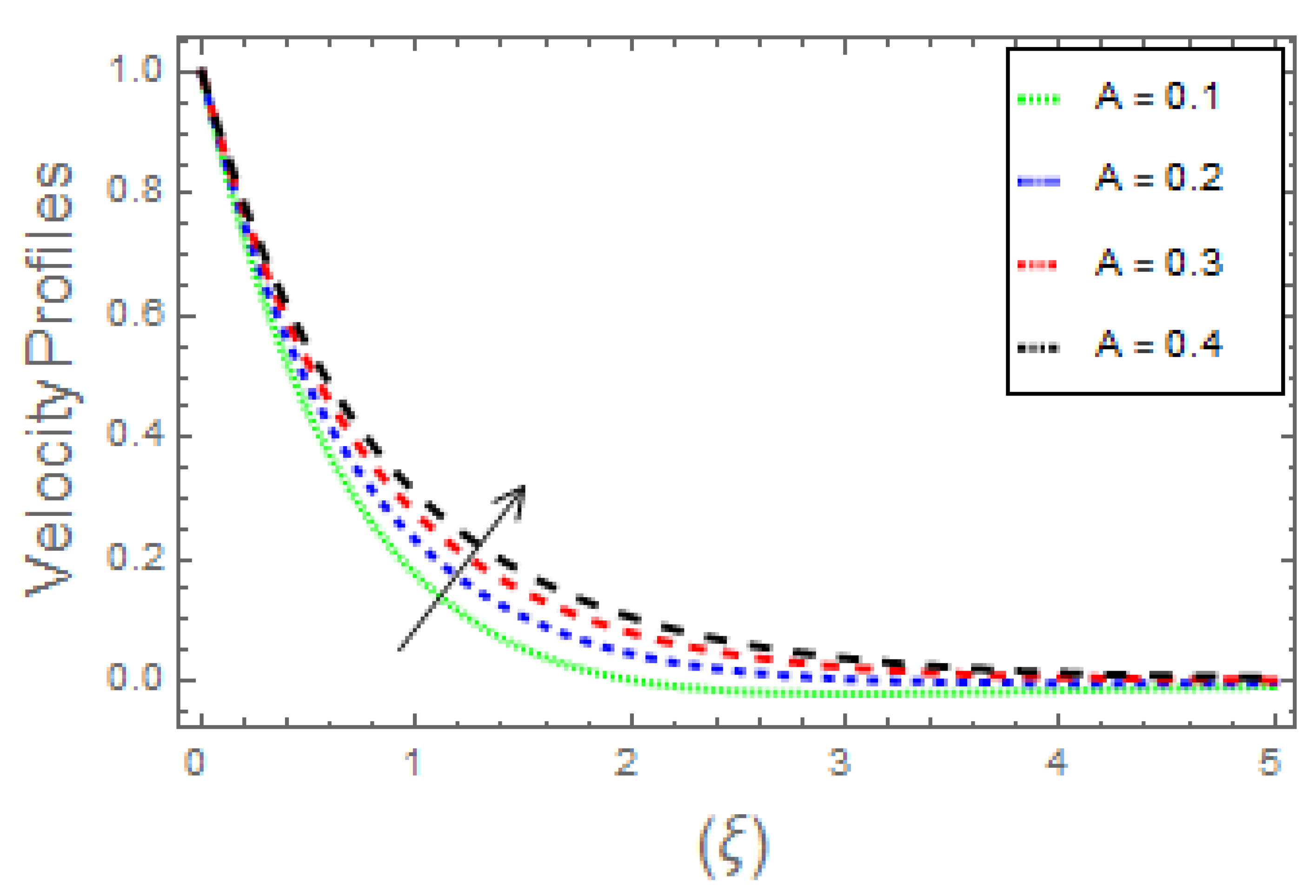
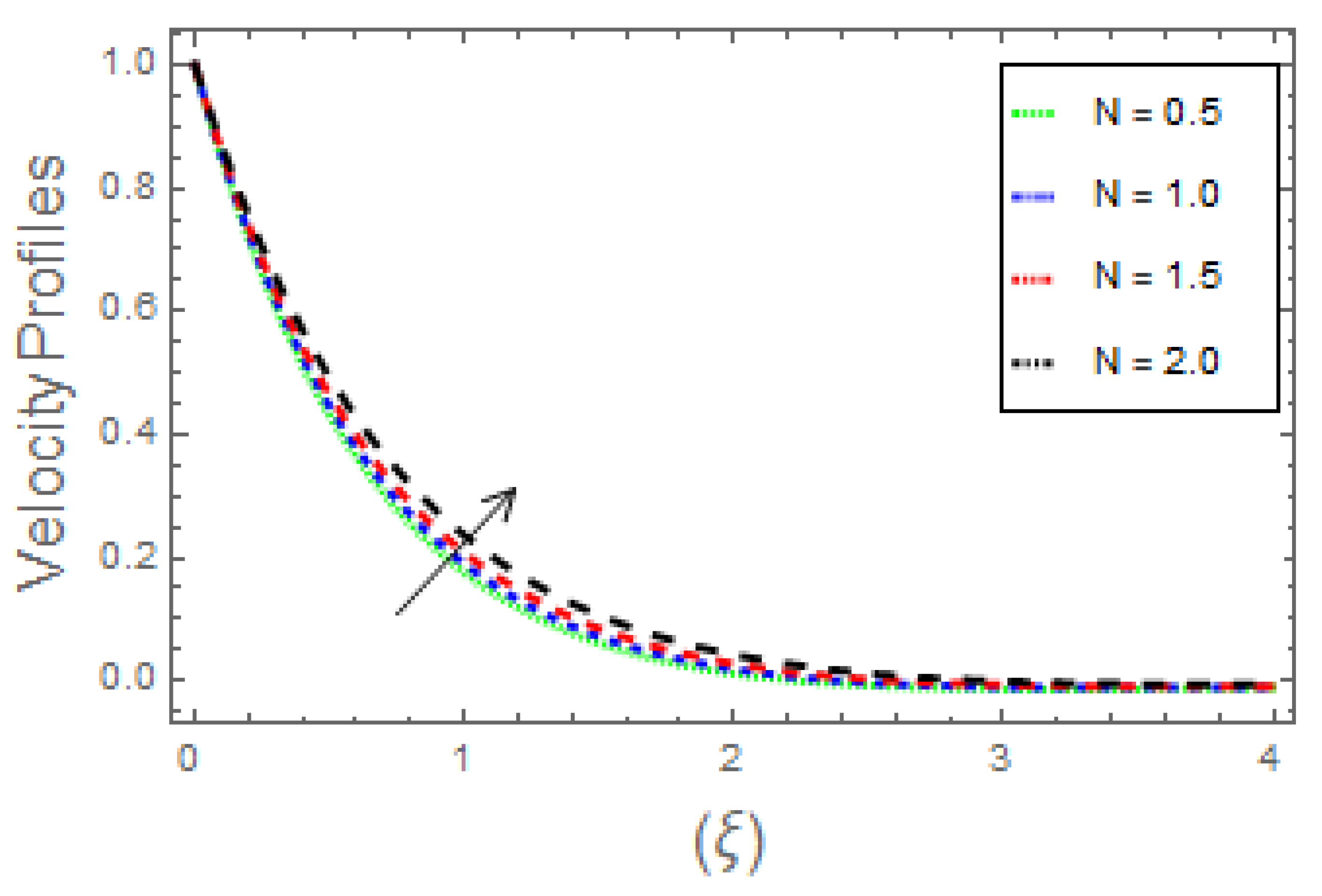
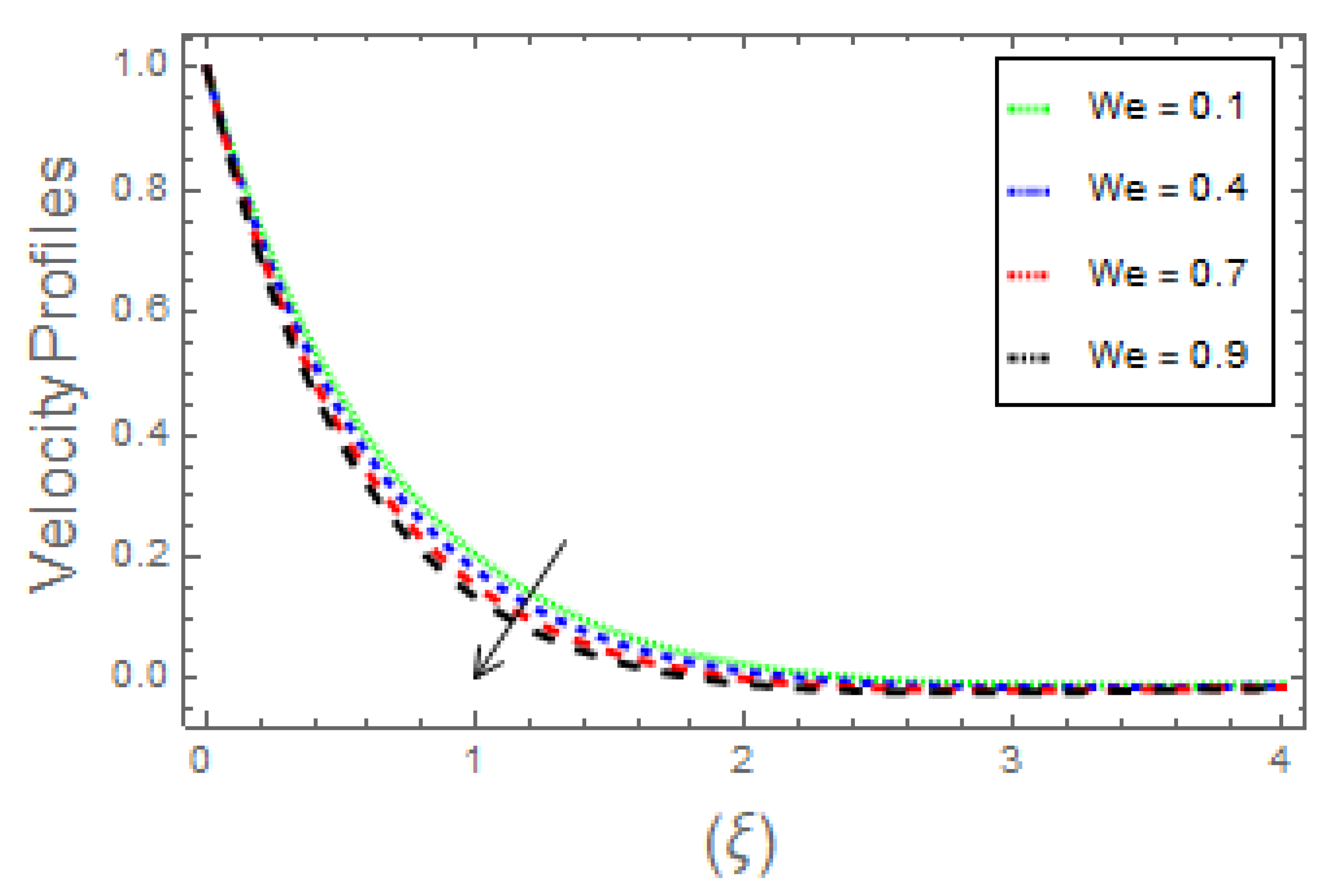
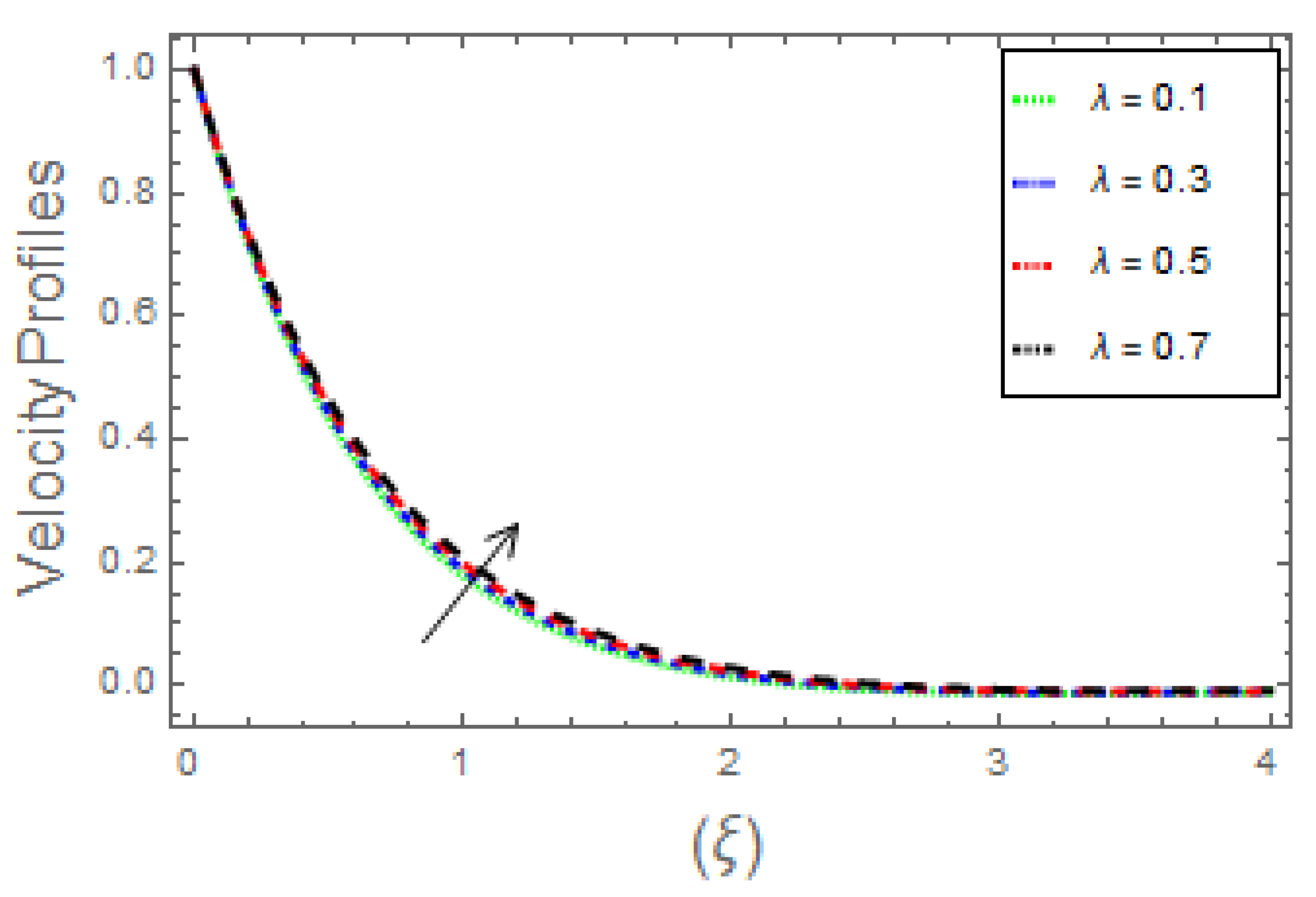
It is observed that boundary layers in $f^{\prime }\left(\xi \right)$ profiles diminish with incrementing data of magnetic parameter and Weissenberg number, whereas increasing the ratio of rate constant parameter, the ratio of thermal to concentration buoyancy forces, and mixed convection parameter caused the $f^{\prime }\left(\xi \right)$ profiles to upsurge;

(2)

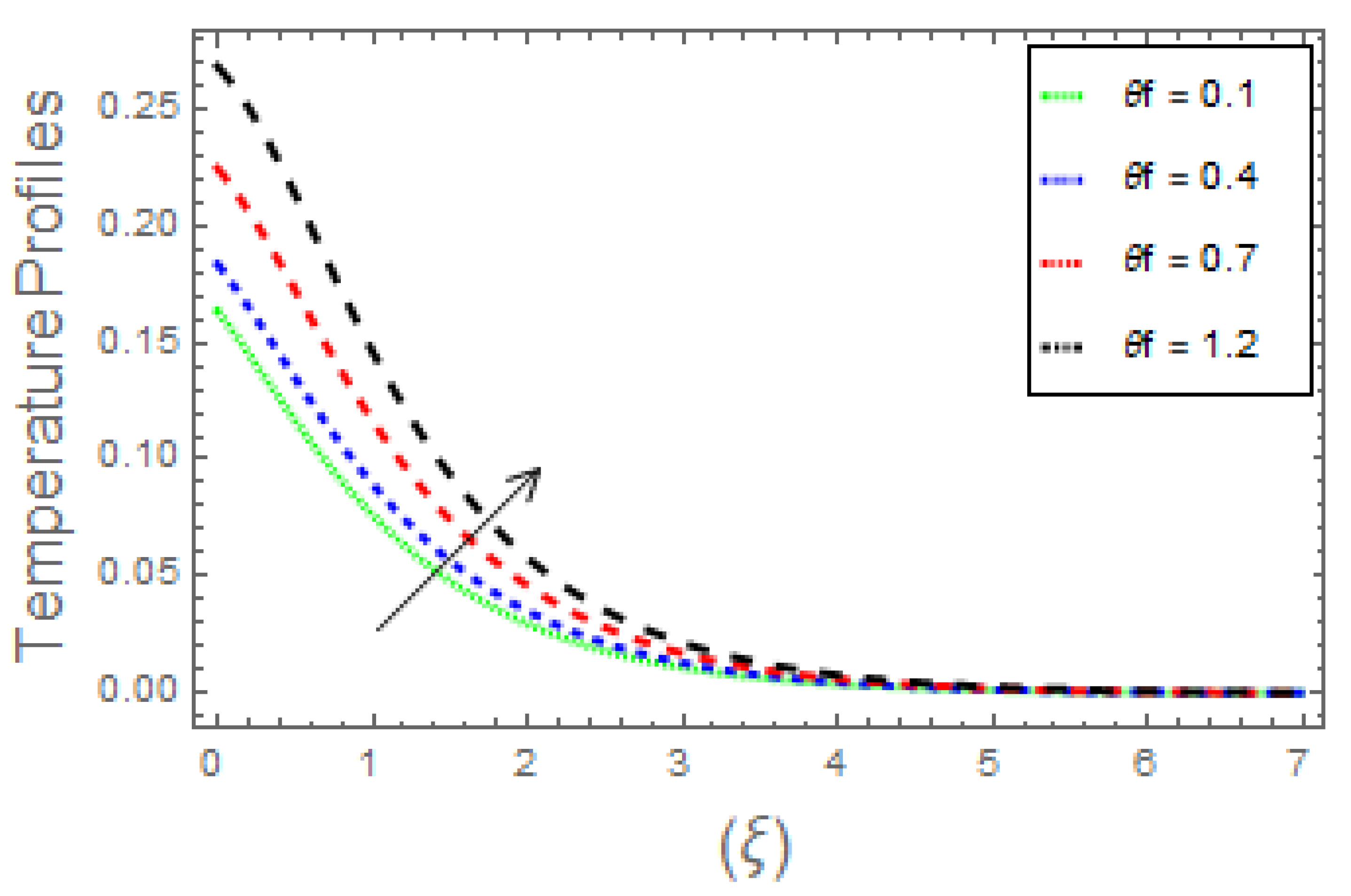
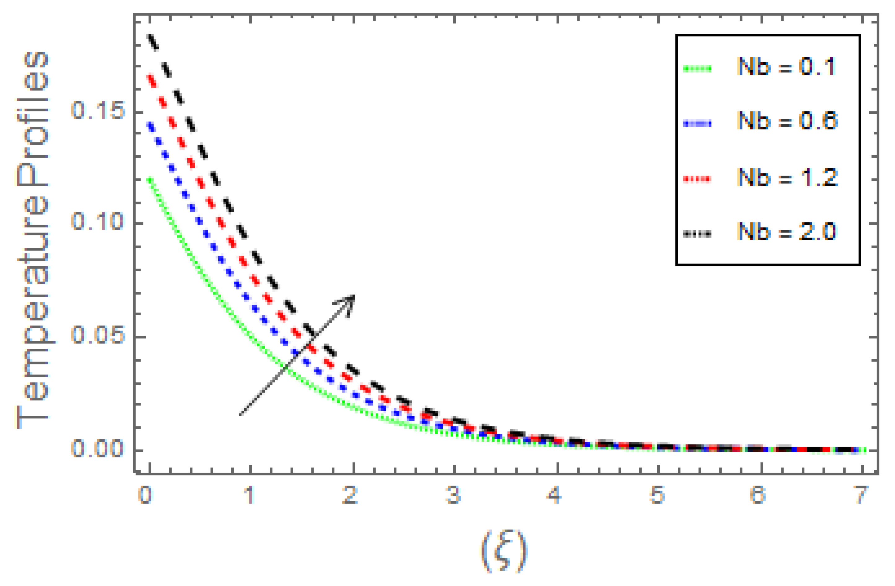
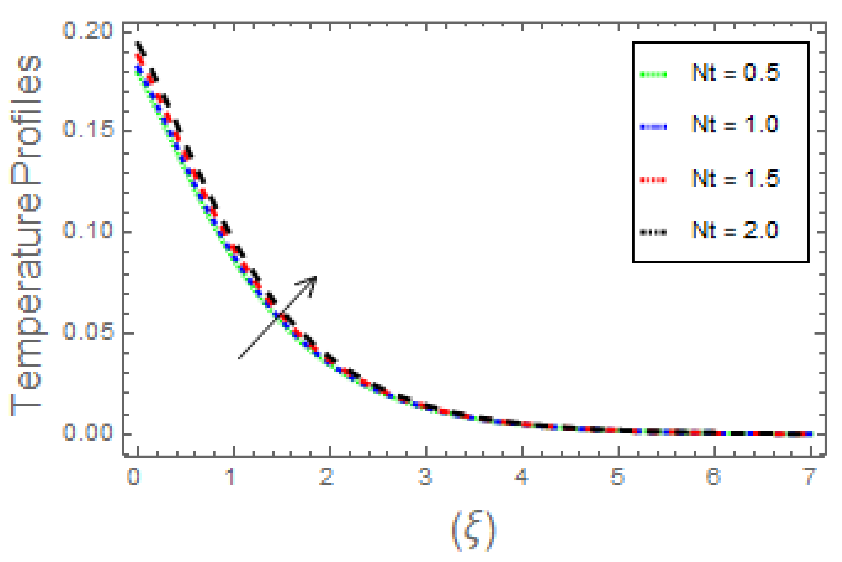
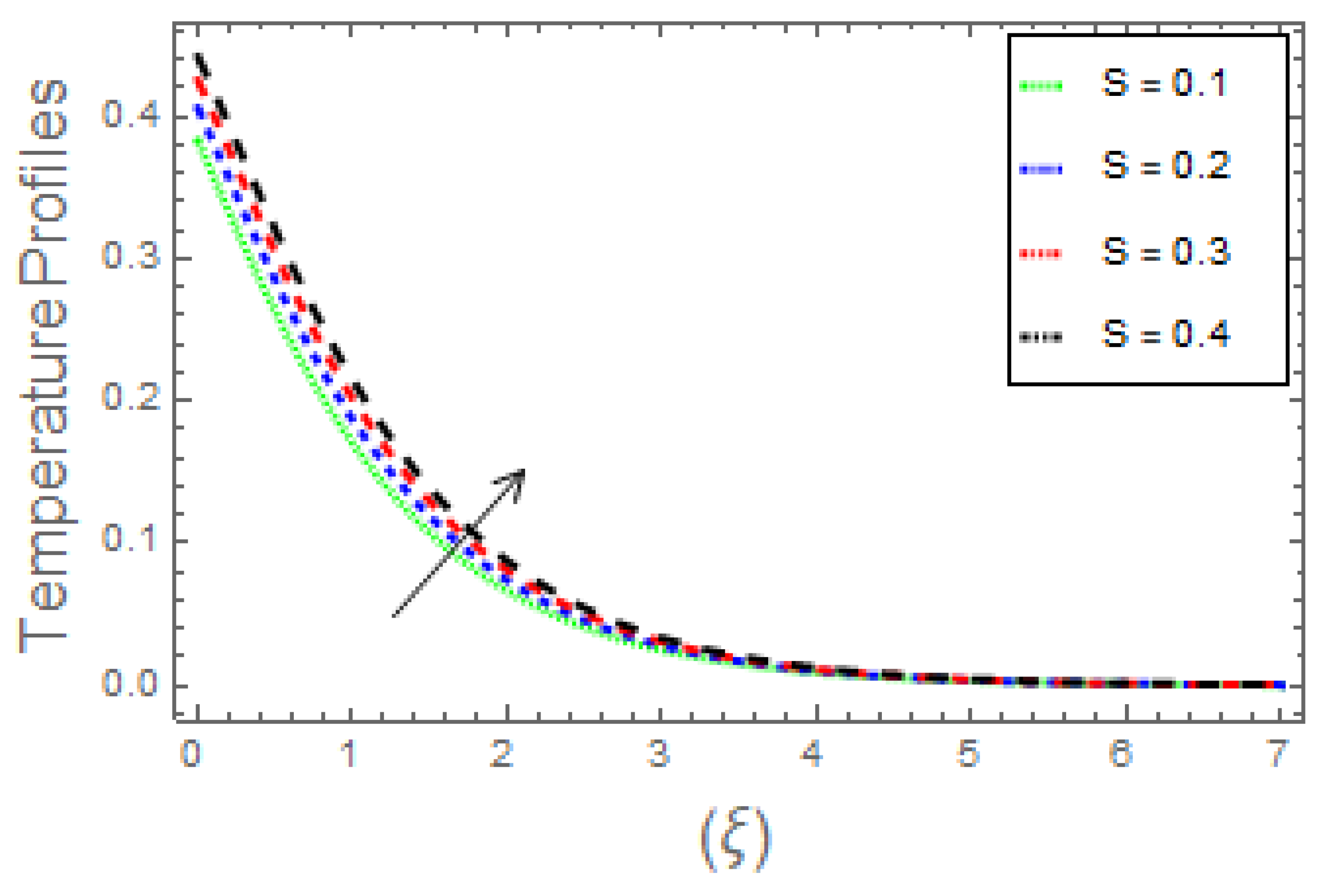
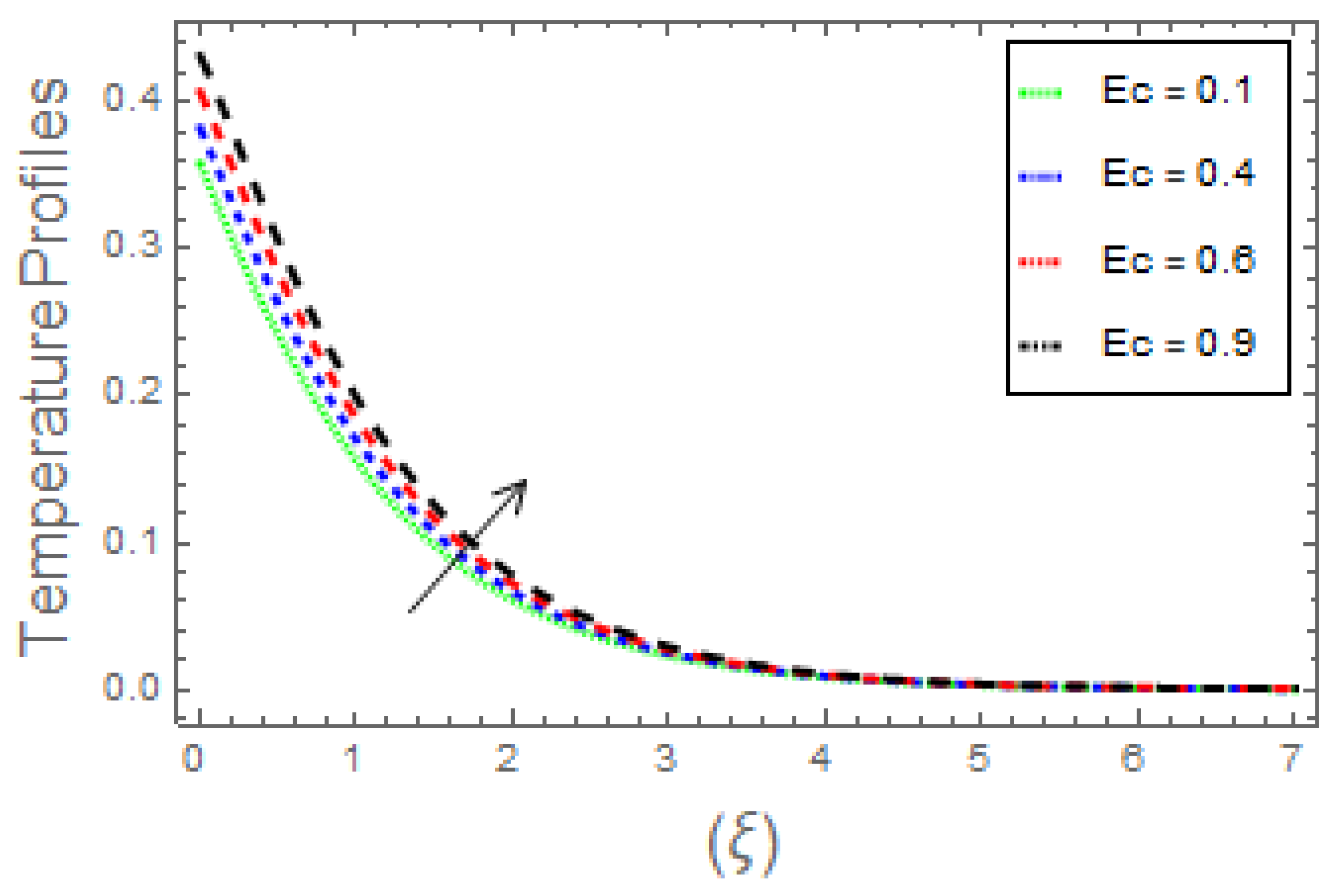
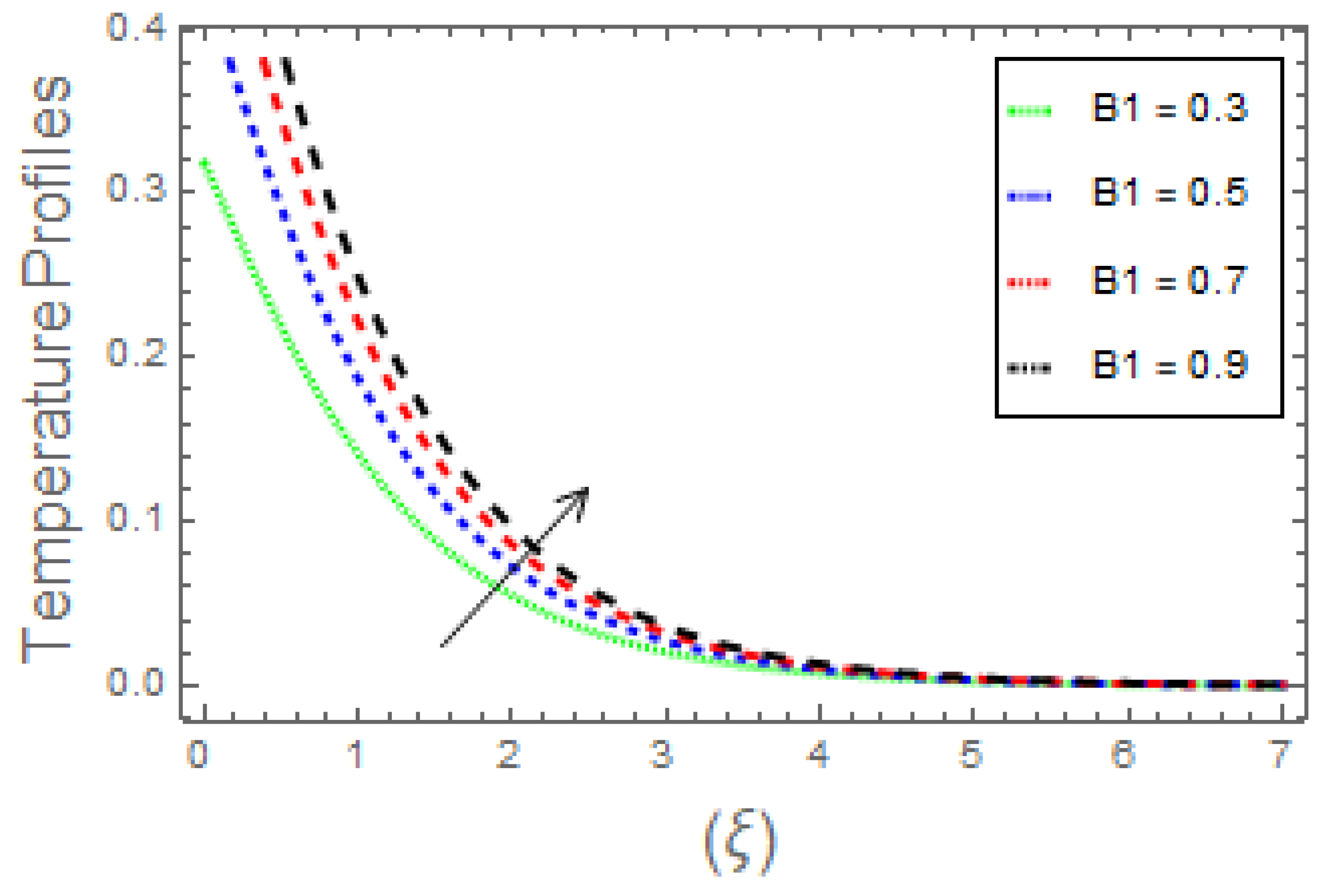
The thermal field curves and heat transfer rates rise due to augmentation in magnetic parameter, radiation factor, heat generation parameter, Eckert number, along with Brownian, thermophoresis, and thermal Biot number. With the upsurge in the Prandtl number, the fluid thermal energy and the related thickness decrease;

(3)

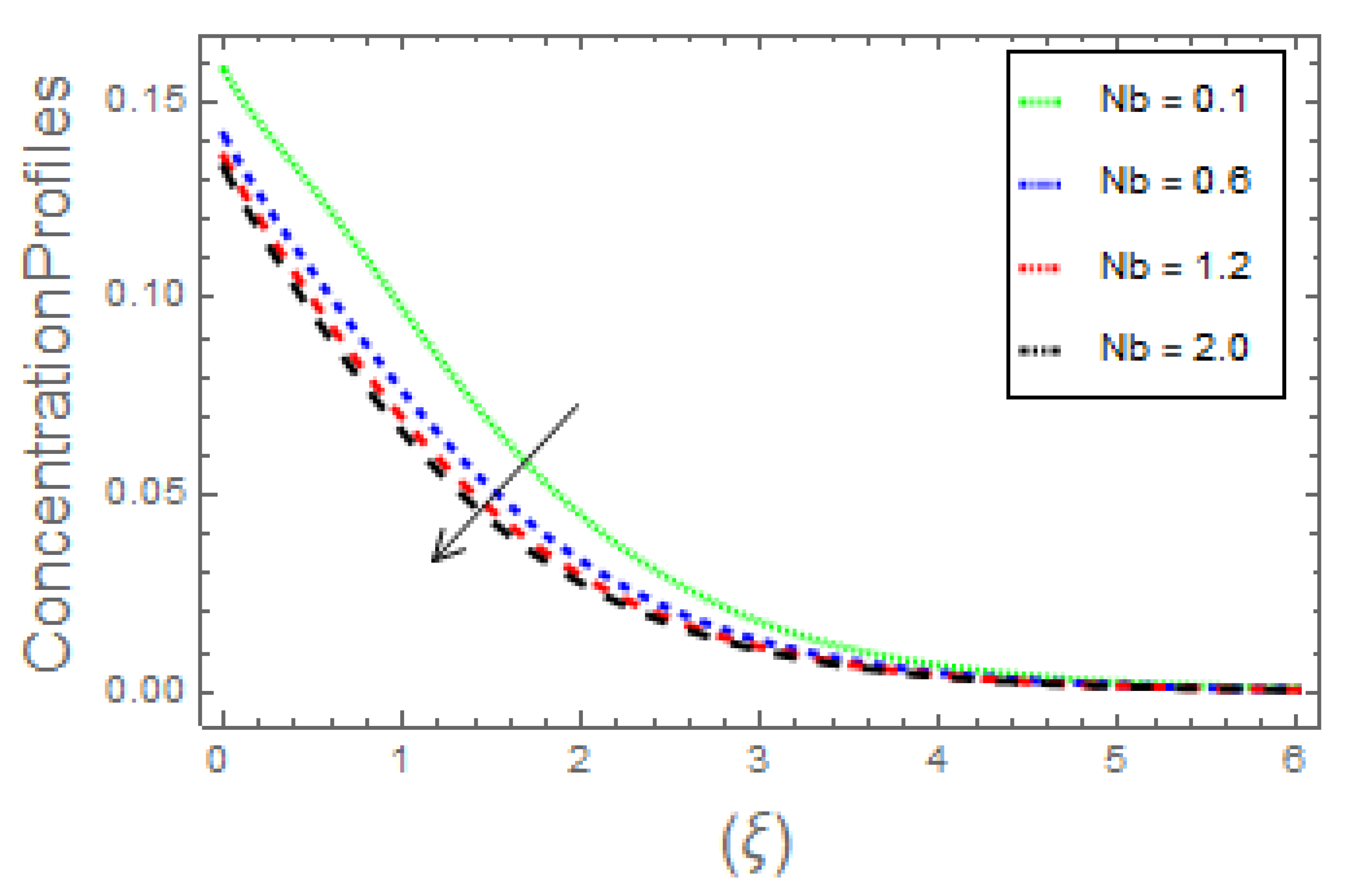
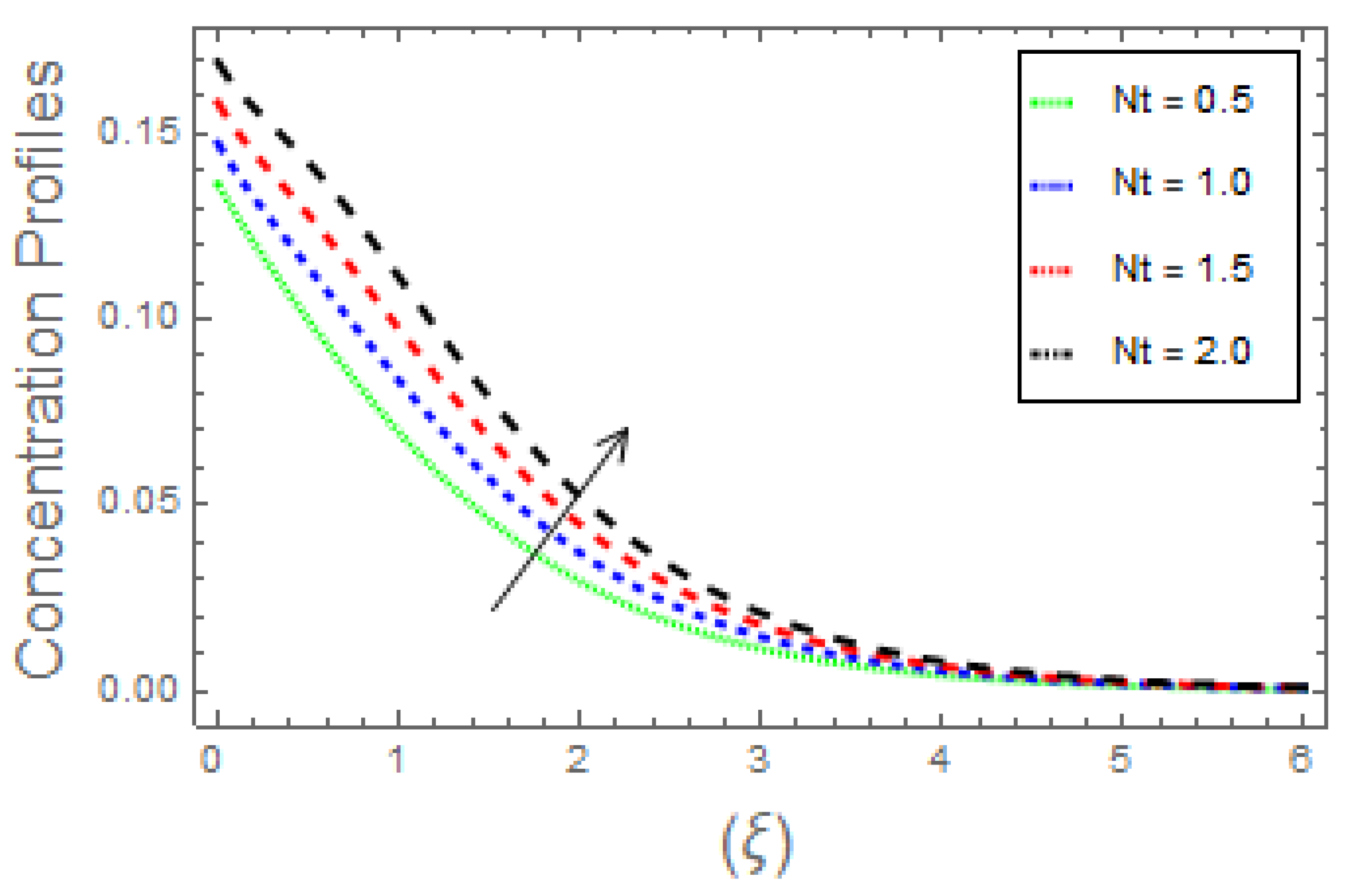
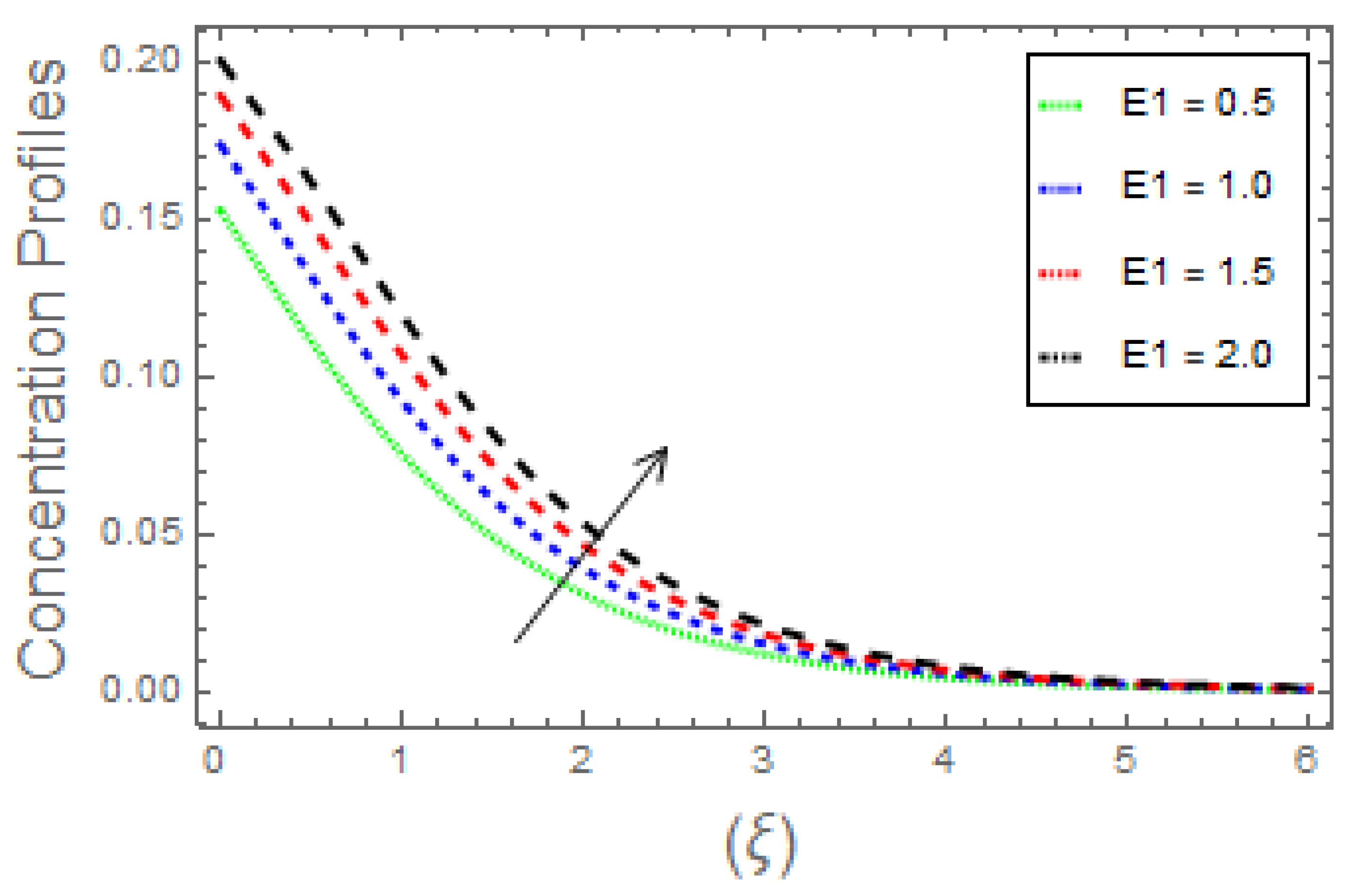
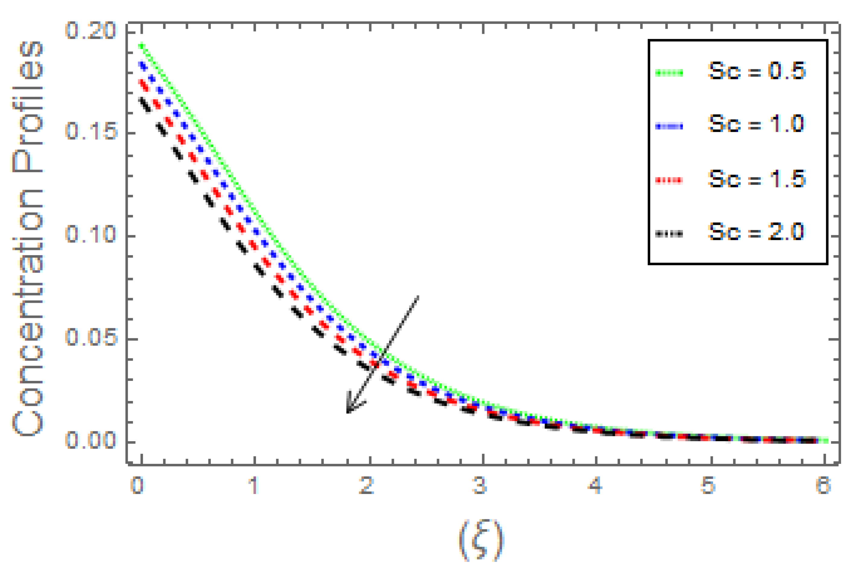
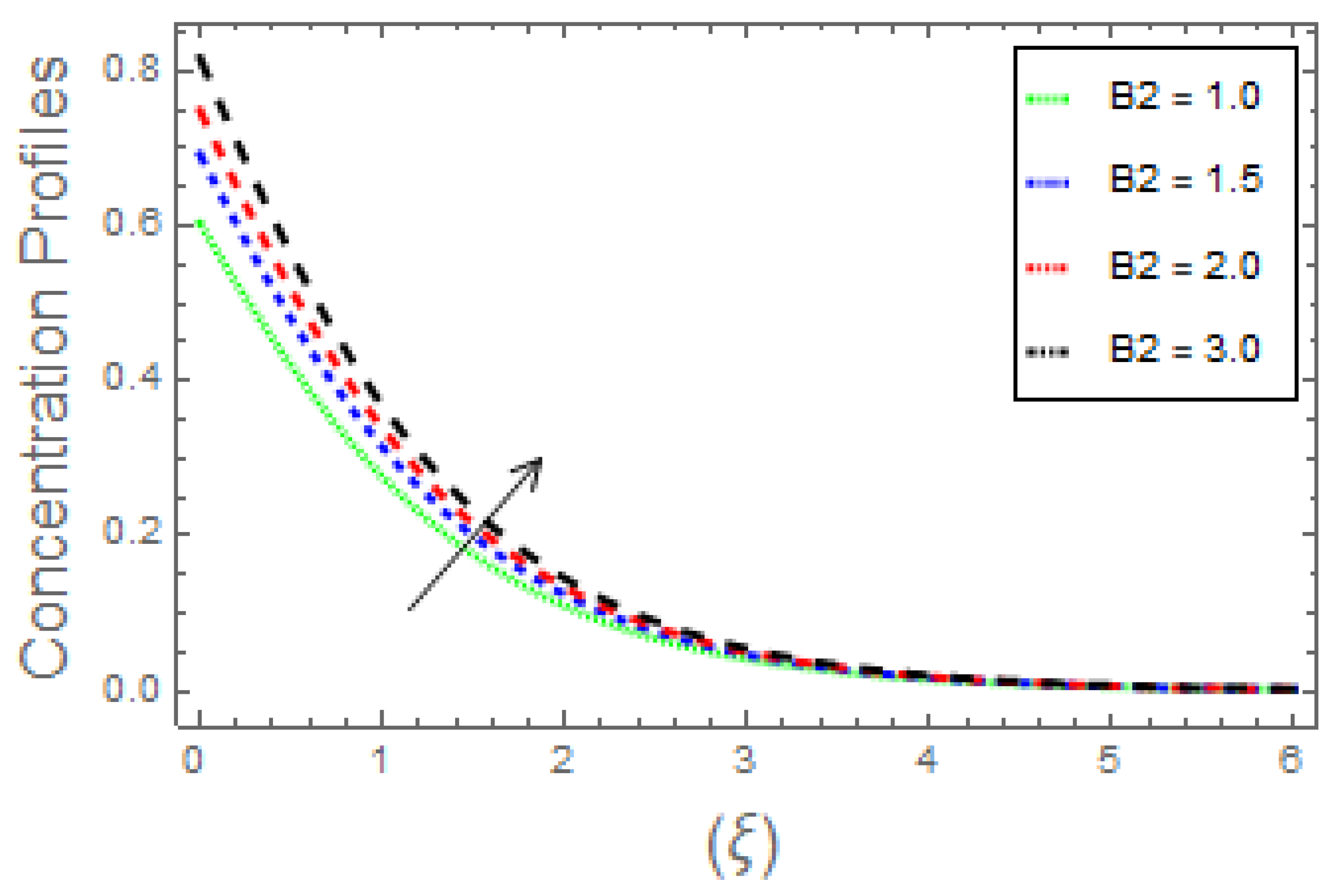
The fluid concentration curves increase owing to increase solutal Biot number, activation energy, and thermophoretic parameter. Moreover, increasing the Brownian parameter and Schmidt number causes the temperature profiles to diminish;

(4)

The surface drag force coefficient $C{f}_x$ enhances with higher data of magnetic and ratio of rate constant parameters;

(5)

It is found that the heat transfer coefficient $N{u}_x$ decays via increasing values of Brownian and thermophoretic parameters;

(6)

An increase in mass flow rate $S{h}_x$ is detected for the increasing values of Schmidt number and Brownian parameter.

References

- Choi, S. Enhancing Thermal Conductivity of Fluids with Nanoparticles; American Society of Mechanical Engineers, Fluids Engineering Division (Publication) FED: New York, NY, USA, 1995; Volume 231, pp. 99–105. [Google Scholar]
- Sarkar, J.; Ghosh, P.; Adil, A. A review on hybrid nanofluids: Recent research, development and applications. Renew. Sustain. Energy Rev. 2015, 43, 164–177. [Google Scholar] [CrossRef]
- Jusoh, R.; Nazar, R.; Pop, I. Dual solutions of magnetohydrodynamic stagnation point flow and heat transfer of viscoelastic nanofluid over a permeable stretching/shrinking sheet with thermal radiation. In Journal of Physics: Conference Series; IOP Publishing: Bristol, UK, 2017. [Google Scholar]
- Rasheed, H.U.; Islam, S.; Noor, S.; Khan, W.; Abbas, T.; Khan, I.; Kadry, S.; Nam, Y.; Nisar, K.S. Impact of magnetohydrodynamics on stagnation point slip flow due to nonlinearly propagating sheet with nonuniform thermal reservoir. Math. Probl. Eng. 2020, 2020, 1794213. [Google Scholar]
- Pal, D.; Mandal, G. Magnetohydrodynamic stagnation point flow of Sisko nanofluid over a stretching sheet with suction. Propuls. Power Res. 2020, 9, 408–422. [Google Scholar] [CrossRef]
- Abbasi, A.; Farooq, W.; Riaz, I. Stagnation point flow of Maxwell nanofluid containing gyrotactic microorganism impinging obliquely on a convective surface. Heat Transf. 2020, 49, 2977–2999. [Google Scholar] [CrossRef]
- Lund, L.A.; Omar, Z.; Khan, I.; Baleanu, D.; Nisar, K.S. Dual similarity solutions of MHD stagnation point flow of Casson fluid with effect of thermal radiation and viscous dissipation: Stability analysis. Sci. Rep. 2020, 10, 1–13. [Google Scholar]
- Sheikholeslami, M.; Farshad, S.A.; Said, Z. Analyzing entropy and thermal behavior of nanomaterial through solar collector involving new tapes. Int. Commun. Heat Mass Transf. 2021, 123, 105190. [Google Scholar] [CrossRef]
- Hsiao, K.L. To promote radiation electrical MHD activation energy thermal extrusion manufacturing system efficiency by using Carreau nanofluid with parameters control method. Energy 2017, 130, 486–499. [Google Scholar] [CrossRef]
- Hsiao, K.L. Stagnation electrical MHD nanofluid mixed convection with slip boundary on a stretching sheet. Appl. Therm. Eng. 2016, 98, 850–861. [Google Scholar] [CrossRef]
- Chakraborty, S.; Panigrahi, P.K. Stability of nanofluid: A review. Appl. Therm. Eng. 2020, 174, 115259. [Google Scholar] [CrossRef]
- Khan, M.I.; Hafeez, M.U.; Hayat, T.; Khan, M.I.; Alsaedi, A. Magneto rotating flow of hybrid nanofluid with entropy generation. Comput. Methods Programs Biomed. 2020, 183, 105093. [Google Scholar] [CrossRef]
- Izadi, A.; Siavashi, M.; Rasam, H.; Xiong, Q. MHD enhanced nanofluid mediated heat transfer in porous metal for CPU cooling. Appl. Therm. Eng. 2020, 168, 114843. [Google Scholar] [CrossRef]
- Atif, S.M.; Hussain, S.; Sagheer, M. MHD micropolar nanofluid with non-Fourier and non-Fick’s law. Int. Commun. Heat Mass Transf. 2021, 122, 105114. [Google Scholar] [CrossRef]
- Sheikholeslami, M.; Farshad, S.A. Investigation of solar collector system with turbulator considering hybrid nanoparticles. Renew. Energy 2021, 171, 1128–1158. [Google Scholar] [CrossRef]
- Atif, S.M.; Hussain, S.; Sagheer, M. Effect of thermal radiation on MHD micropolar Carreau nanofluid with viscous dissipation, Joule heating, and internal heating. Sci. Iran. 2019, 26, 3875–3888. [Google Scholar] [CrossRef] [Green Version]
- Rasheed, H.U.; Islam, S.; Khan, Z.; Khan, J.; Mashwani, W.K.; Abbas, T.; Shah, Q. Computational analysis of hydromagnetic boundary layer stagnation point flow of nano liquid by a stretched heated surface with convective conditions and radiation effect. Adv. Mech. Eng. 2021, 13, 16878140211053142. [Google Scholar] [CrossRef]
- Hayat, T.; Waqas, M.; Shehzad, S.A.; Alsaedi, A. Mixed convection flow of viscoelastic nanofluid by a cylinder with variable thermal conductivity and heat source/sink. Int. J. Numer. Methods Heat Fluid Flow 2016, 2, 214–234. [Google Scholar] [CrossRef]
- Ramesh, G.K.; Gireesha, B.J. Influence of heat source/sink on a Maxwell fluid over a stretching surface with convective boundary condition in the presence of nanoparticles. Ain Shams Eng. J. 2014, 5, 991–998. [Google Scholar] [CrossRef] [Green Version]
- Khan, M.; Khan, W.A.; Alshomrani, A.S. Non-linear radiative flow of three-dimensional Burgers nanofluid with new mass flux effect. Int. J. Heat Mass Transf. 2016, 101, 570–576. [Google Scholar] [CrossRef]
- Mahanthesh, B.; Gireesha, B.J.; Gorla, R.S.R.; Abbasi, F.M.; Shehzad, S.A. Numerical solutions for magnetohydrodynamic flow of nanofluid over a bidirectional non-linear stretching surface with prescribed surface heat flux boundary. J. Magn. Magn. Mater. 2016, 417, 189–196. [Google Scholar] [CrossRef]
- Hayat, T.; Waqas, M.; Khan, M.I.; Alsaedi, A. Analysis of thixotropic nanomaterial in a doubly stratified medium considering magnetic field effects. Int. J. Heat Mass Transf. 2016, 102, 1123–1129. [Google Scholar] [CrossRef]
- Hayat, T.; Waqas, M.; Shehzad, S.A.; Alsaedi, A. On model of Burgers fluid subject to magneto nanoparticles and convective conditions. J. Mol. Liq. 2016, 222, 181–187. [Google Scholar] [CrossRef]
- Farooq, M.; Khan, M.I.; Waqas, M.; Hayat, T.; Alsaedi, A.; Khan, M.I. MHD stagnation point flow of viscoelastic nanofluid with non-linear radiation effects. J. Mol. Liq. 2016, 221, 1097–1103. [Google Scholar] [CrossRef]
- Arrhenius, S. On the reaction rate of the inversion of non-refined sugar upon souring. Z. Phys. Chem. 1889, 4, 226. [Google Scholar] [CrossRef] [Green Version]
- Ren, Z.; Lei, Z.; Li, C.; Xuan, W.; Zhong, Y.; Li, X. New study and development on electromagnetic field technology in metallurgical processes. Acta Metall. Sin. 2020, 56, 583–600. [Google Scholar]
- Hsiao, K.L. Combined electrical MHD heat transfer thermal extrusion system using Maxwell fluid with radiative and viscous dissipation effects. Appl. Therm. Eng. 2017, 112, 1281–1288. [Google Scholar] [CrossRef]
- Naz, R.; Noor, M.; Hayat, T.; Javed, M.; Alsaedi, A. Dynamism of magnetohydrodynamic Cross nanofluid with particulars of entropy generation and gyrotactic motile microorganisms. Int. Commun. Heat Mass Transf. 2020, 110, 104431. [Google Scholar] [CrossRef]
- Atif, S.M.; Hussain, S.; Sagheer, M. Heat and mass transfer analysis of time-dependent tangent hyperbolic nanofluid flow past a wedge. Phys. Lett. A 2019, 283, 1187–1198. [Google Scholar] [CrossRef]
- Qayyum, S.; Hayat, T.; Shehzad, S.A.; Alsaedi, A. Effect of a chemical reaction on magnetohydrodynamic (MHD) stagnation point flow of Walters-B nanofluid with newtonian heat and mass conditions. Nucl. Eng. Tech. 2017, 49, 1636–1644. [Google Scholar] [CrossRef]
- Rasheed, H.; AL-Zubaidi, A.; Islam, S.; Saleem, S.; Khan, Z.; Khan, W. Effects of Joule Heating and Viscous Dissipation on Magnetohydrodynamic Boundary Layer Flow of Jeffrey Nanofluid over a Vertically Stretching Cylinder. Coatings 2021, 11, 353. [Google Scholar] [CrossRef]
- Islam, S.; Haroon, R.; Kottakkaran, S.N.; Nawal, A.A.; Mohammed, Z. Numerical Simulation of Heat Mass Transfer Effects on MHD Flow of Williamson Nanofluid by a Stretching Surface with Thermal Conductivity and Variable Thickness. Coatings 2021, 11, 684. [Google Scholar] [CrossRef]
- Rasheed, R.; Islam, S.; Khan, Z.; Alharbi, S.O.; Khan, W.A.; Khan, W.; Khan, I. Thermal Radiation Effects on Unsteady Stagnation Point Nanofluid Flow in View of Convective Boundary Conditions. Math. Probl. Eng. 2021, 2021, 5557708. [Google Scholar] [CrossRef]
- Rasheed, H.; Islam, S.; Khan, Z.; Alharbi, S.O.; Alotaibi, H.; Khan, I. Impact of Nanofluid Flow over an Elongated Moving Surface with a Uniform Hydromagnetic Field and Nonlinear Heat Reservoir. Complexity 2021, 2021, 9951162. [Google Scholar] [CrossRef]
- Liao, S.J. Homotopy Analysis Method in Nonlinear Differential Equations; Higher Education Press: Berlin/Heidelberg, Germany; Shanghai, China, 2012; p. 200030. [Google Scholar]
- Liao, S. Beyond Perturbation: Introduction to the Homotopy Analysis Method; CRC Press: Boca Raton, FL, USA, 2003. [Google Scholar]
- Liao, S.J. An optimal homotopy-analysis approach for strongly nonlinear differential equations. Commun. Nonlinear Sci. Numer. Simul. 2010, 15, 2003–2016. [Google Scholar] [CrossRef]
- Alolaiyan, H.; Riaz, A.; Razaq, A.; Saleem, N.; Zeeshan, A.; Bhatti, M.M. Effects of Double Diffusion Convection on Third Grade Nanofluid through a Curved Compliant Peristaltic Channel. Coatings 2020, 10, 154. [Google Scholar] [CrossRef] [Green Version]
- Liao, S. On the homotopy analysis method for nonlinear problems. Appl. Math. Comput. 2004, 147, 499–513. [Google Scholar] [CrossRef]