1. Introduction
As well as in the laboratory and on earth, fullerenes have been found in a range of nonterrestrial environments [
1,
2,
3,
4,
5,
6,
7,
8,
9,
10]. Recent confirmation that C
60+ is the source of some of the strong diffuse interstellar bands (DIBs) [
5,
11] suggests that fullerenes may play a key astrochemical role. However, the formation mechanisms of fullerenes in such extreme environments are still a debated question. Interestingly, while one might intuitively expect hydrogen to stabilise dangling bonds at edge sites and hence promote the formation of polyaromatic hydrocarbons rather than fullerenes, astrochemists have recently found that C
60 and C
70 are abundant in hydrogen-containing stars [
8,
9,
12,
13]. This suggests that hydrogen may play a role in fullerene growth. As such, stable hydrogenated small fullerenes are potentially of interest in astrochemistry, both as species in their own right and/or as degradation products from polyaromatic hydrocarbons [
14], and as intermediates in the formation processes of larger fullerenes.
The stability of fullerenes strongly depends on the arrangement of pentagons and hexagons. According to the isolated pentagon rule (IPR), structures composed of isolated pentagons surrounded by five hexagons are favoured by the strain delocalisation and bonding [
15]. The smallest fullerene to fully obey the IPR is the highly stable C
60, Buckminster fullerene. Fullerenes smaller than C
60 are increasingly unstable due to steric strain originating within the non-IPR structures, and bond frustration in areas of high nonplanarity. One route to potentially stabilise local strain and under-coordination is chemical functionalisation of the most reactive carbon sites. For example, while pure C
50 appears unstable, C
50Cl
10 has been isolated and characterised [
16], and the stability and lifetime of C
20 is greatly enhanced when fully hydrogenated to C
20H
20 [
17]. This suggests that the relative stability of smaller fullerenes may be modified in the presence of hydrogen. While there has been extensive experimental [
13,
18,
19,
20,
21] and theoretical [
13,
18,
22] studies of hydrogenated C
60, less attention has been given to smaller hydrogenated fullerenes. It was theoretically proposed that
Td-C
28H
4, a tetrahedral fullerene with triply fused pentagons on each corner of the tetrahedron, might be stable [
15] and indeed has since been experimentally identified [
23]. For smaller fullerenes, an in silico investigation suggested that fused-pentagon sites are preferred in general for single hydrogen addition [
24].
Exploring the landscape of smaller hydrogenated fullerenes is potentially a highly complex and computationally intensive task. Very little can necessarily be determined in advance: neither the hydrogenation sites on the fullerene surface, nor the number of hydrogen additions–nor even the most stable carbon isomer for hydrogenation. This results in a vast and generally intractable number of potential calculations.
Considering first the number of pentagon and hexagon carbon fullerenes smaller than C
60, there is only 1 isomer for each of C
20, C
24, and C
26, and 2 for C
28. However, this rapidly increases, reaching 40 isomers for C
40, and 437 for C
52. In total, there are 3958 C
x pentagon-hexagon fullerenes with x < 60 [
25].
Considering now hydrogenation, if symmetry is not taken into account, then for a single fullerene Cn, there are n possible addition sites for a first hydrogen atom. However, this increases rapidly as more sites are hydrogenated. For two hydrogen atoms, there are n(n−1)/2 arrangements (divided by two as the hydrogens are interchangeable), and in general, for m hydrogen atoms, there are n!/(n−m)!m! arrangements. Thus, for C28H5, this gives 98,280 possible structures, and for larger hydrogenated species such as C50H4, there are 230,300 possibilities. While symmetry can help reduce these numbers, they remain highly challenging for standard density functional theory (DFT) calculations, where it can take several minutes on a state-of-the-art desktop PC to geometrically optimise even the smallest fullerene C20. As we do not, in principle, know how many hydrogen atoms are likely to bind to a given isomer, we would be required to start with single hydrogenation and then increase the number of hydrogen atoms sequentially until the hydrogen binding energy becomes too low.
As the time cost for a brute force approach using DFT to this problem is not possible, it was the aim of the current study to explore, test, and validate different possible methods that might be used to reduce the complexity of this problem and render it accessible computationally. This includes assumptions on growth sequence, the use of geometric and electronic parameters as guides towards selecting the most reactive sites for functionalisation, and the use of different computational approximations such as empirical potentials and tight binding methods to increase calculation speed. We started with a sequence of DFT calculations and used these thereafter as our benchmark energies for the subsequent studies.
2. Method
Coordinates for the fullerene cage structures were taken from Yoshida’s fullerene library [
26]. Geometric analysis of the fullerenes was performed using the
pychemcurv python libraries discussed further in Ref [
27].
All DFT calculations were carried out under the local density approximation (LDA) using the AIMPRO code [
28,
29,
30]. Pseudo-potentials were given by Hartwigsen, Goedecker, and Hutter (HGH) [
31]. Wavefunctions were handled using a basis set of Gaussian-type orbitals [
32,
33], in which 38 (12) functions were used for carbon (hydrogen) atoms. Charge density was handled using plane waves. Spin averaging was used for systems with an even number of electrons. Spin polarisation was used with a spin excess of 1.0 for systems with an odd number of electrons. An additional spin excess of either 0.1 or 1.0 was added when charge was added while exploring frontier orbitals. Charged systems were handled by introducing a uniform homogenous compensating background charge to the cell. The smearing of electronic occupations using a Fermi function with an effective temperature of 0.04 eV was set during the geometry optimisation procedure. All molecules were modelled in face-centred cells with a
0 = 15.875 Å to ensure negligible inter-fullerene interactions. Structures were geometrically optimised until the system energy was converged within 10
−5 Ha, and positions to within 10
−4 a
0.
The LDA was selected based on previous experience with graphite, where it regularly outperformed GGA [
34]. Quantum Monte Carlo calculations (including London dispersion) showed that errors are closely correlated to the Laplacian (neglected in density functionals), rather than the gradient of the electron density [
35]. Model systems showed some cancellation of errors for the LDA; however, GGA construction can magnify rather than reduce this error. LDA provides a better description of interlayer binding in graphite than GGAs [
34], supported by random phase approximation (RPA) calculations [
36], and shows better G-band frequency shifts with doping than the GGA [
37]. In practice, in the current systems, this choice between LDA and GGA-PBE does not matter, as, when we geometrically optimised over 700 hydrogenated fullerene structures with both functionals and compared energies, the result was a fully linear fit (see
Supplementary Materials Figure S4). As the energies are thus directly proportional, the comparative results in the current study will also be directly transferable to GGA studies.
Empirical potential calculations were performed using the LAMMPS code [
38], using the REBO [
39], AIREBO [
40], and AIREBO-M [
41] potentials. In each case, the structures were optimised with a 10
−10 convergence threshold (ratio of energy change to total energy magnitude), at zero Kelvin. The reactive empirical bond order (REBO) is a potential developed by Brenner [
39]. REBO is handled by a Tersoff-type potential [
42,
43], which deals with the formation and deformation of covalent bonds during a calculation and was developed for hydrogen [
44] and carbon [
44,
45]-containing systems. The adaptive intermolecular reactive empirical bond order (AIREBO) potential [
40] was developed for carbon-hydrogen systems. It uses REBO to describe nonbonded interactions. In this study, we included its torsion term and the Lennard–Jones (LJ) cut-off radius set at 2.5 (in σ scale factor). AIREBO-M is a hybrid potential of AIREBO and Morse [
41]. In this potential, a LJ term in AIREBO is replaced with a Morse potential parameterised to Møller–Plesset method (MP2) calculations [
46,
47]. In this study, we included its torsion term and the Morse cutoff radius set at 3.0 (in σ scale factor).
Semi-empirical molecular orbital calculations were performed using MOPAC2016 [
48] as implemented in the OpenMOPAC code. Default options were taken, except the MOZYME option that was selected, a method developed for quick calculations of organic molecules that replaces the self-consistent field (SCF) method with a localised molecular orbital (LMO) method. Different semi-empirical parameterisations were tested, namely PM6 + D3, PM7, and RM1. PM6 [
49] was fitted to reference data from DFT calculations and was combined here with Grimme’s D3 method for longer-range dispersion interactions [
50]. For PM7, geometric and enthalpy errors were improved compared to PM6 [
49] by reconsidering new reference data [
51]. In this method, a D2 correlation was combined to take into account the dispersion. The correlation term was based on the exchange-correlation functional of the generalised gradient approximation (GGA). Finally, RM1 [
52] was developed from AM1 [
53] by improved parameters. It utilises different equations from PM6 to consider the core–core interactions.
The semi-empirical extended tight binding method (xTB) as implemented in GFN2-xTB is a quantum calculation method for gas and condensed phases developed by Grimme and co-workers [
54]. It covers a large number of elements up to radon and is based on DFT perturbation expansion of the electron density, which makes it applicable to electronically complicated systems. For a large number of isomers of fullerene C
60, xTB has already shown excellent structure–energy agreement with DFT results with Pearson’s correlation coefficient r = 0.998 [
55]. Again, we used default settings including for convergence cut-offs.
3. Results
3.1. Pure Carbon Fullerenes
Using DFT-LDA, we first optimised all pure-carbon isomers of C
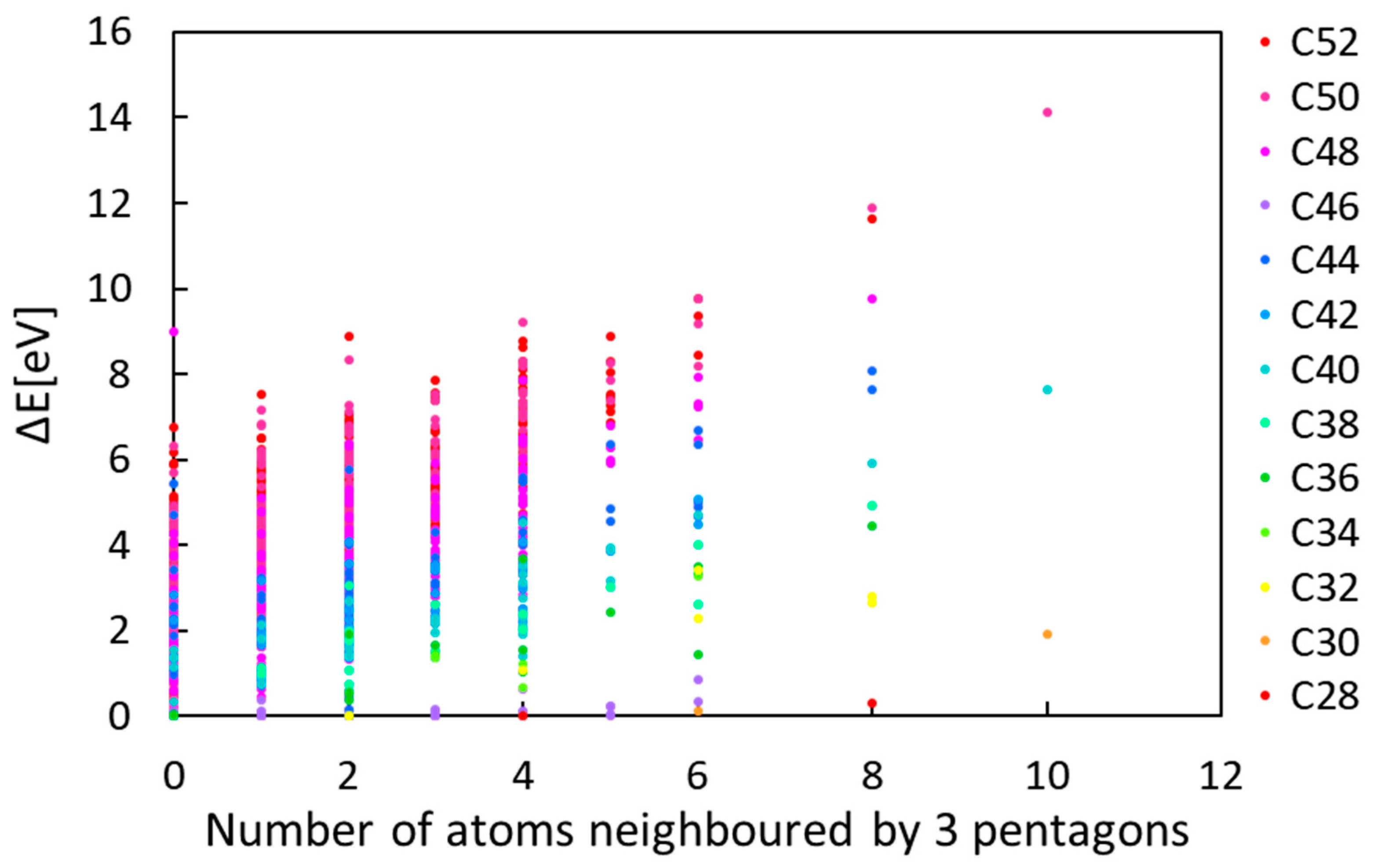
x fullerenes from x = 28 to x = 52, a total of 1246 structures.
Figure 1 shows on the y-axis the energy difference between a given isomer and the most stable isomer for the same number of carbon atoms. On the x-axis, we give the number of atoms in the isomer neighbouring three pentagons. This plot confirms the general tendency that the stability of a given fullerene is negatively proportional to the number of triple-fused pentagons, although there are a number of interesting exceptions.
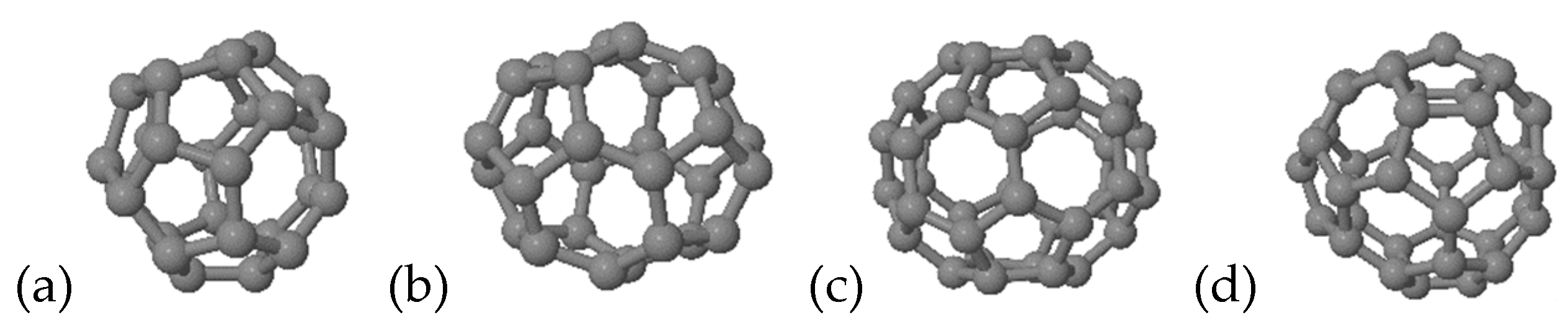
For the following hydrogenation study, we focused on only four representative structures, C
28 (1-
Td and 2-
D2, index of Yoshida’s library [
26]-symmetry symbol) and C
40 (38-
D2 and 40-
Td) (see
Figure 2). These were chosen as the
Td tetrahedral structures have four, the maximum number, triple-fused pentagons, and the other structures are the lowest-energy pure-carbon structures in each isomer group.
3.2. First Hypothesis—Sequential Hydrogen Addition
In order to tackle the problem of the calculation time cost, our first hypothesis is that hydrogen atoms bind sequentially, in each case, to the most stable site, and thereafter do not move. Such an approach was shown to successfully predict stable fluorinated fullerene [
56], fullerene chlorination [
57], and functionalisation with CF
3 groups [
58,
59]. This reduces the number of calculations substantially. To determine the stable structure of C
nH
m, we first geometrically optimised the system C
nH with hydrogen in each of the
n possible sites. We took the most stable solution and fixed the first hydrogen at this site, tested the
n − 1 possible sites for the next hydrogen, and so on. As an example, for C
28H
5, this reduces the number of calculations from 98,280 to 130, and for C
50H
4 from 230,300 to 194, with the additional benefit that the stable structures for C
nH, C
nH
2, etc. are automatically determined as part of the process.
While the method works well for halogens where the binding energies are high, its validity for hydrogenation is less clear. This hypothesis for sequential hydrogenation is tested in
Section 3.3 and
Section 3.4 below. In the current section, we employ sequential addition for our benchmark DFT calculations, exploring hydrogenation up to
m = 5, i.e., C
28H
5 and C
40H
5.
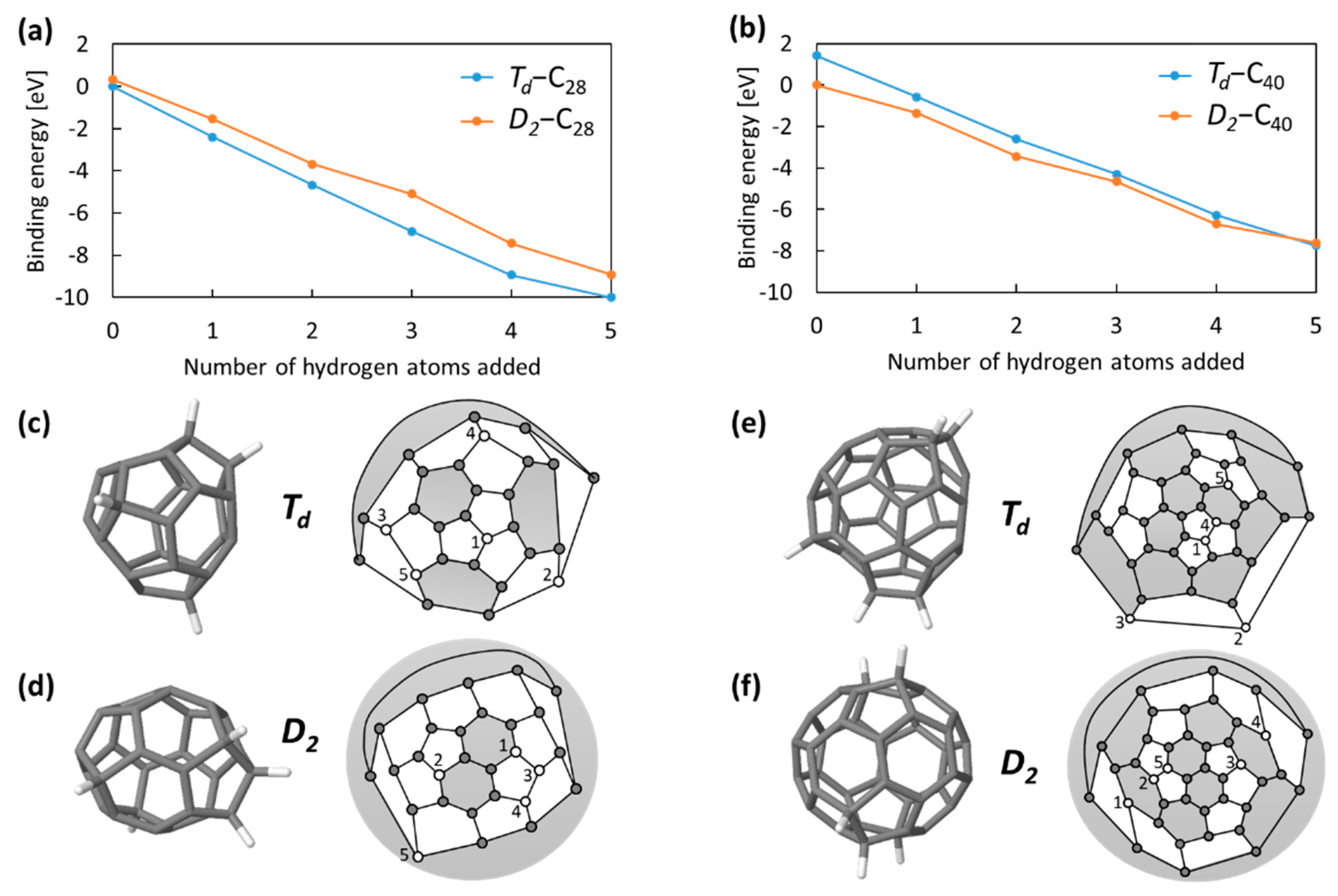
Figure 3 shows the structures obtained this way for C
28H
5 and C
40H
5 for the two
Td and
D2 isomers. The energy axis shows the total binding energy of the hydrogen, calculated as
where C
n is the fullerene in question and C
n′ is the energetically most stable isomer fullerene. The projected Schlegel diagrams are marked numerically with the hydrogen addition sequence.
Td-C
28 is sequentially hydrogenated at each triple pentagon on the tetrahedral corner sites, with the fifth hydrogenation occurring with a lower binding energy visible as a change in the total energy gradient. At each stage, this is the stable C
28 isomer. In contrast, the stable C
40 isomer is the lower-symmetry
D2-C
40. Subsequent hydrogenation occurs around the “caps” of this isomer. When the binding energies are normalised by the number of hydrogen atoms added, we see a general convergence towards hydrogen binding of ~1.6 eV for the
D2-C
40 isomer, with higher binding (~2.0 eV) for the
Td-C
28, consistent with its smaller size and lower aromaticity.
Hydrogen binds more strongly to the Td-C40 isomer than the D2-C40 (although it does not, this time, adopt the triple-pentagon tetrahedrally symmetric sites). This lowers the relative energy difference between the isomers until, at C40H5, there is a transition and the Td-C40H5 isomer becomes the most stable. This demonstrates that the most stable pure carbon isomer cannot be taken as a guide in general for which the hydrogenated isomer will be stable, i.e., wider isomer testing is required.
3.3. Second Hypothesis—Predicting Reactive Sites via Local Geometry
The first hypothesis of sequential addition still requires every possible addition site to be geometrically optimised for each fullerene isomer, and it is desirable to reduce this further. In the section hypothesis, we postulate that the most reactive site for hydrogenation on a given fullerene might be determined in advance from the local geometry of the fullerene before the hydrogen is added. If this hypothesis is correct, it allows the prediction in advance of which site will be hydrogenated next, in principle, reducing the number of calculations for C28H5, for example, from 130 to simply 5.
There are a number of geometric parameters that have been explored in the literature as a way of indicating local site reactivity in fullerenes, most of which have been discussed at a good level of detail in Reference [
27]. In general, they all try to quantify in some way the degree to which the
pz-orbital of the carbon atom is able to form a strong π-bond with one or more of its neighbours, typically through some measure of local curvature. In the following, we selected one geometric criterion and calculated its value for all nonhydrogenated sites on a given fullerene cage. The most extreme value (minimum or maximum, as discussed below) was taken as the next site to hydrogenate. The new structure was then geometrically optimised using DFT, and the process repeated. In this way, a hydrogenation sequence can be built up with geometric site selection at each step, and this sequence can be compared to the “lowest-energy” sequence derived in
Section 3.2.
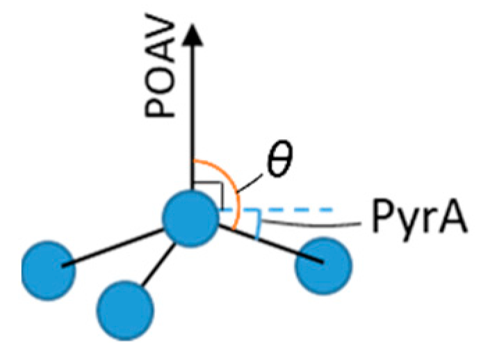
We first tested the pyramidalization angle (PyrA). This is defined as θ-π/2, where θ is the angle between the π-orbital axis vector (POAV) and a vector from a central atom to a side atom (except the atom along POAV), as shown in
Figure 4 [
60,
61,
62]. The POAV is defined as a vector at constant angle to the three carbon-carbon bonds [
63]. Thus, in a flat graphene sheet, the pyrA is zero. A further derivative from pyrA is the hybridisation value defined by Haddon [
60,
61,
62] and explored further by Sabalot-Cuzzubbo and colleagues [
11]. This is essentially a more chemical reworking of the pyrA in terms of the amount of s
xp
y character in the system. For both of these parameters, we calculated the values for all potential binding sites and selected the maximum for hydrogenation at each step.
An alternative geometric approach is to use bond lengths rather than angles. The idea behind this simple geometric test is that decreasing the π-bond character of an atom will tend to result in longer, purely single-character bonds, and hence a highly reactive radical should have three long single bonds. In the three-bond sum geometric parameter, we simply sum the three bond lengths between a central atom and its adjacent atoms and hydrogenate the atom with the largest three-bond sum. A refinement of the three-bond sum model is a two-bond sum. In principle, in a strongly localised but nonaromatic π-bound atom, it is possible to have one short double bond and two long single bonds in aromatic bonds, which may nonetheless result in a high three-bond sum. The two-bond sum model tries to avoid this by eliminating the shortest bond and hydrogenating the atom with the lowest sum of the remaining two bond lengths.
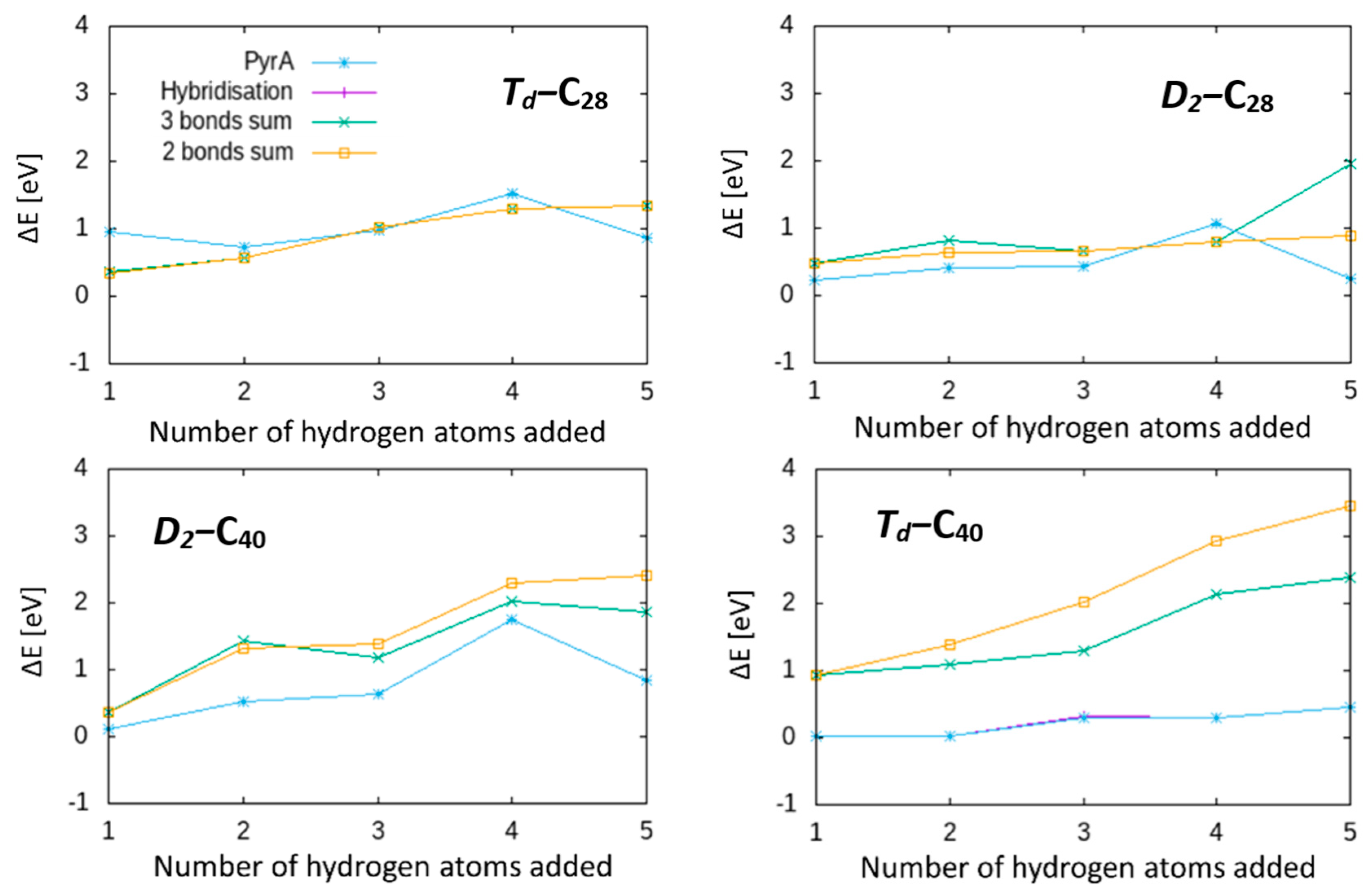
In each of these four cases, we followed the hydrogen addition sequence and compared the energy of the DFT-optimised structure with that found from testing all available sites at each addition step from
Section 3.2 (
Figure 5, Schlegel projections showing hydrogenation sites shown in
Figure S1). As expected, hybridisation and pyrA give the same hydrogenation sequence. While these two parameters find the lowest-energy structures for
Td-C
40H and
Td-C
40H
2, in general, none of these geometric methods correctly select the lowest-energy hydrogenation sites, that is, none are capable of predicting the DFT-predicted most-stable structures.
3.4. Third Hypothesis—Predicting Reactive Sites via Local Electronic Structure
Instead of using local geometry, we next considered potential hydrogenation site selection rules based on the local electronic structure of the parent molecule. It might be imagined that the site with the most local pz-orbital character will release the most energy when hydrogenated. Alternatively, in cases where there is charge redistribution (notably on partially hydrogenated cages), sites showing excessive charging may also be targets for hydrogenation. We tested a number of electronic possibilities to select the next site for hydrogenation.
The simplest is to consider local Mulliken charges as determined by a Mulliken population analysis, as an estimate of atomic charge distribution in a molecule [
64]. Hydrogenating the atom showing the highest Mulliken charge results in the sequence shown in
Figure 5 (blue trace, Schlegel projections in
Figure S1), where the lowest energy pathway is clearly not selected. A more sophisticated approach is to use frontier orbitals [
65]. In this case, we add or remove some charge to the system, and by taking the difference in Mulliken values between the charged and neutral molecule, we identify where this charge is localising and can use that as an indication of local site reactivity. Such an approach doubles the number of geometric optimisations required, as for each fullerene, a second optimisation of the charged species is required, but this remains a tractable approach compared to the more “brute force” testing approaches described above. In essence, adding some charge gives an indication of the localisation of the lowest unoccupied molecular orbital (LUMO), with the benefit of geometric optimisation allowing the system to respond to the charge state change.
In the following, we tested two charging values, adding either 0.1e or a full electron to the system. Frontier orbital values for individual atoms were determined as the difference between the calculated Mulliken charge for the atom when the molecule was charged, and the Mulliken charge for that atom in the neutral system. Thus, the lowest Frontier orbital value in the system indicates that for the atom that accumulates the most charge when the 0.1/1e is added to the whole system, the highest Frontier orbital value is the atom that accumulates the least (or indeed loses the most charge if the frontier orbital value is positive). Once the site is chosen, we hydrogenate this atom and continue with geometric optimisation in the neutral charge state as before. We tried the following sequences of both the lowest and highest frontier orbital values.
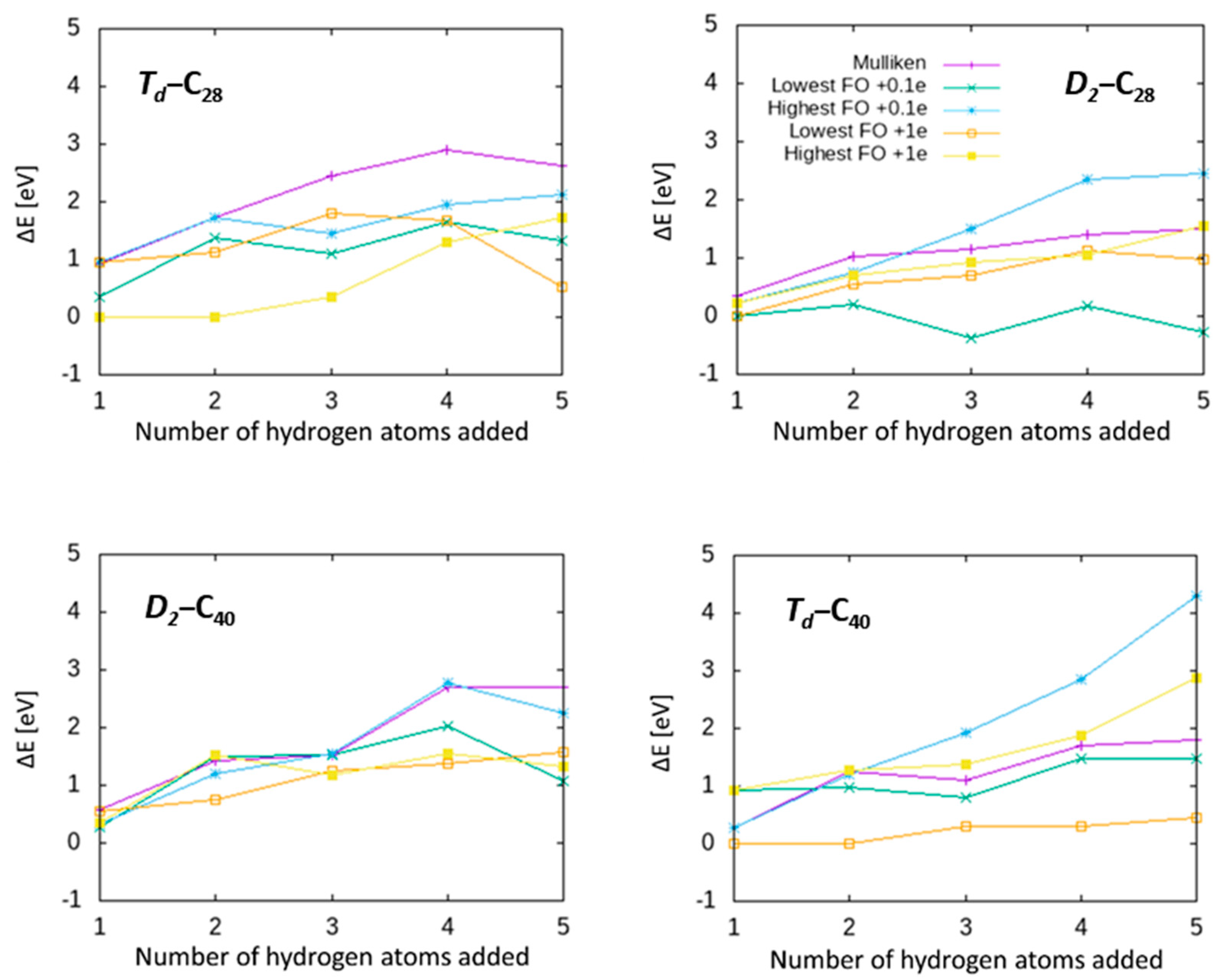
The results are shown in
Figure 6 (Schlegel projections in
Figure S1). In general, the frontier orbital values perform better than the simple Mulliken charges as a guide, and most give more stable isomers than the geometric parameters tested above. Nonetheless, none of them are able to systematically reproduce the low-energy structures obtained through sequential addition in
Section 3.2. Thus, we have demonstrated that the hypotheses of predicting hydrogenation sites on small fullerenes using the geometric and electronic parameters tested are not valid, i.e. these do not provide reliable routes to predicting hydrogenated structures directly from the parent fullerenes.
It is worth examining the Frontier orbital data for
D2-C
28 in more detail, as it reveals another important result. It can be seen that when considering the lowest Frontier orbital atoms for hydrogenation, in the case of adding only 0.1
e, for
D2-C
28H
3 and
D2-C
28H
5, the addition sequence actually predicts hydrogenated isomers that are
more stable than those obtained in
Section 3.2. This is important as it invalidates our first hypothesis, namely that sequential hydrogen addition always generates the lowest-energy hydrogenated fullerenes. The implication is that if hydrogen can rearrange on the fullerene surface as further hydrogen atoms are added, this has the potential to lower the system energy. It is difficult to say whether kinetic barriers will limit this process under laboratory conditions; while calculations for single hydrogen migration suggest relatively high barriers [
24], in practice, a range of barriers will exist depending on local geometry, degree of hydrogen surface coverage, and local environment. In interstellar environments where UV-photon absorption is the primary interaction event [
14], structural rearrangement is likely.
Thus, we have demonstrated that none of the three proposed hypotheses provide a valid route to simplifying structure selection for hydrogenated fullerenes. This leaves a potentially intractable problem given the large number of hydrogenated fullerenes that need testing, and the associated time for each DFT calculation. The next approach is therefore to try and reduce the computational cost of the calculations.
To finish this section, we note that another possible route for functionalisation site prediction based on electronic structure is via local aromaticity, in particular, through the calculation of nucleus-independent chemical shifts (NICS) for each ring in the system [
66]. This has previously been successfully applied to fullerene hydrogenation [
67] and fluorination [
56]. Positive (negative) NICS values indicate less (more) aromatic rings, and the values for three rings surrounding a given atom can be used as an indication of the degree of aromaticity of that site. We did not follow that approach here, as we have shown above that systematic addition routes do not necessarily lead to system ground state structures, but it would be interesting for a future study to explore whether aromaticity can be a useful tool for determining hydrogenation magic numbers.
3.5. Second Strategy, Semi-Empirical and Empirical Routes
Rather than applying selection rules to simplify the problem and then using high-level, but slow, DFT tools, an alternative approach is to not simplify the problem but instead tackle every possible hydrogenated fullerene and simplify instead the tool used to make the calculation time acceptable. We used our extensive collection of DFT calculations from
Section 3.2 as a comparative benchmark. We tested the four representative structures using the following methods: empirical potentials using LAMMPS [
38], semi-empirical molecular orbital approaches using MOPAC [
48], and a relatively new semi-empirical extended tight binding method (GFN2-xTB). GFN2-xTB has previously shown excellent structure–energy agreement with DFT results for C
60 isomers, with Pearson’s correlation coefficient r = 0.998 [
55].
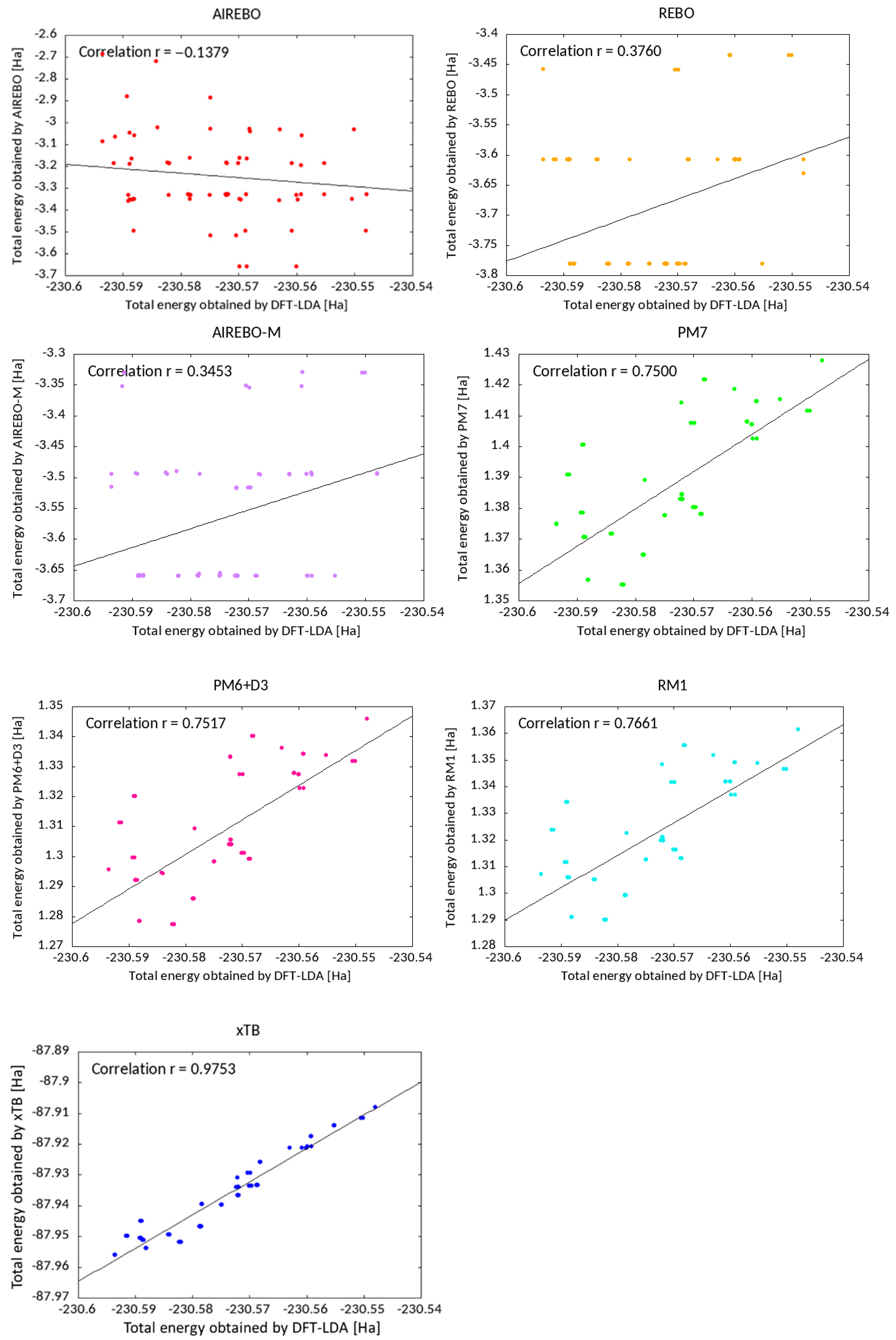
In each case, we geometrically optimised the structure using the method described and then plotted the calculated total energy against that calculated using DFT-LDA. The results are shown for C
40H
5 in
Figure 7, along with the corresponding Pearson’s correlation coefficient. Plots for two other fullerenes (C
28H
5 and C
40H) are shown in
Figures S1 and S2.
The empirical potential-based methods (REBO, AIREBO, and AIREBO-M) show essentially no correlation (r < 0.4) with the DFT-LDA energies. In contrast, the MOPAC semi-empirical-based methods show the same overall energetic stability tendency as DFT, with correlation in the range r = 0.75~0.77. All three methods show a very similar distribution of points. However, in the all three cases, the most stable structure by DFT does not correspond to that obtained by the semi-empirical methods, and indeed lies someway off (for C40H5, using PM7, PM6 + D3, and RM1, the structure predicted by DFT-LDA to be the most stable structure is only 20th on a list of 72). Thus, even if these methods were used to pre-screen suitable structures and a cut-off were applied (with full DFT-LDA geometric optimisation of only the most stable RM1 structures), the cut-off would necessarily have to be quite high, at least 30% of structures, in order to ensure that the lowest-energy DFT-LDA structure was included.
In strong contrast to the above methods, GFN2-xTB shows outstandingly good correlation (r = 0.98) in energetic stability compared to DFT-LDA. Enlarging the lowest-energy range, there is a data cluster, and the lowest-energy structure in DFT shows the lowest energy also by the GFN2-xTB calculation isolated from the other close data points. For other simpler fullerenes (less hydrogenated and a smaller cage), the correlation is even better (
Figures S1 and S2), r = 0.993–0.998.
Table 1 shows the calculated energy difference between the ground-state structure and the next most stable (symmetry nonequivalent) structure for C
28H
n and C
40H
n,
n = 1…5, calculated using DFT-LDA and GFN2-xTB. In each case, GFN2-xTB predicts the same structure ordering amongst the isomers tested, with very close energy differences (standard deviation of 0.087 eV).
If we compare calculation times for these different methods, the potential advantages are clear. The average run-time of each calculation for pure C
20 on a 16-core desktop PC is summarised in
Table 2 (along with the corresponding r-values from
Figure 7). As expected, the empirical potentials are fastest but show no correlation to the DFT-LDA total energies. Of the semi-empirical methods, GFN2-xTB shows by far the best run time, as well as gives the best correlation to DFT-LDA. These results show that we can safely switch to using GFN2-xTB, as it is able to successfully generate DFT-LDA accuracy in total energies of hydrogenated smaller fullerenes, but at over 600 times less computational time.
3.6. All Combination of Hydrogenation Sites Testing by xTB
Next, we tested all the possible combinations of hydrogenation sites up to the 4th hydrogenation using GFN2-xTB for the four fullerene structures discussed above,
Td-C
28,
D2-C
28,
Td-C
40, and
D2-C
40. This brute force approach calculates the total energy for all hydrogen isomers of fullerenes C
nH
m, unlike the sequential test described in
Section 3.2. As such, it provides a definitive lowest-energy hydrogenation sequence for C
nH
m,
m = 0…4.
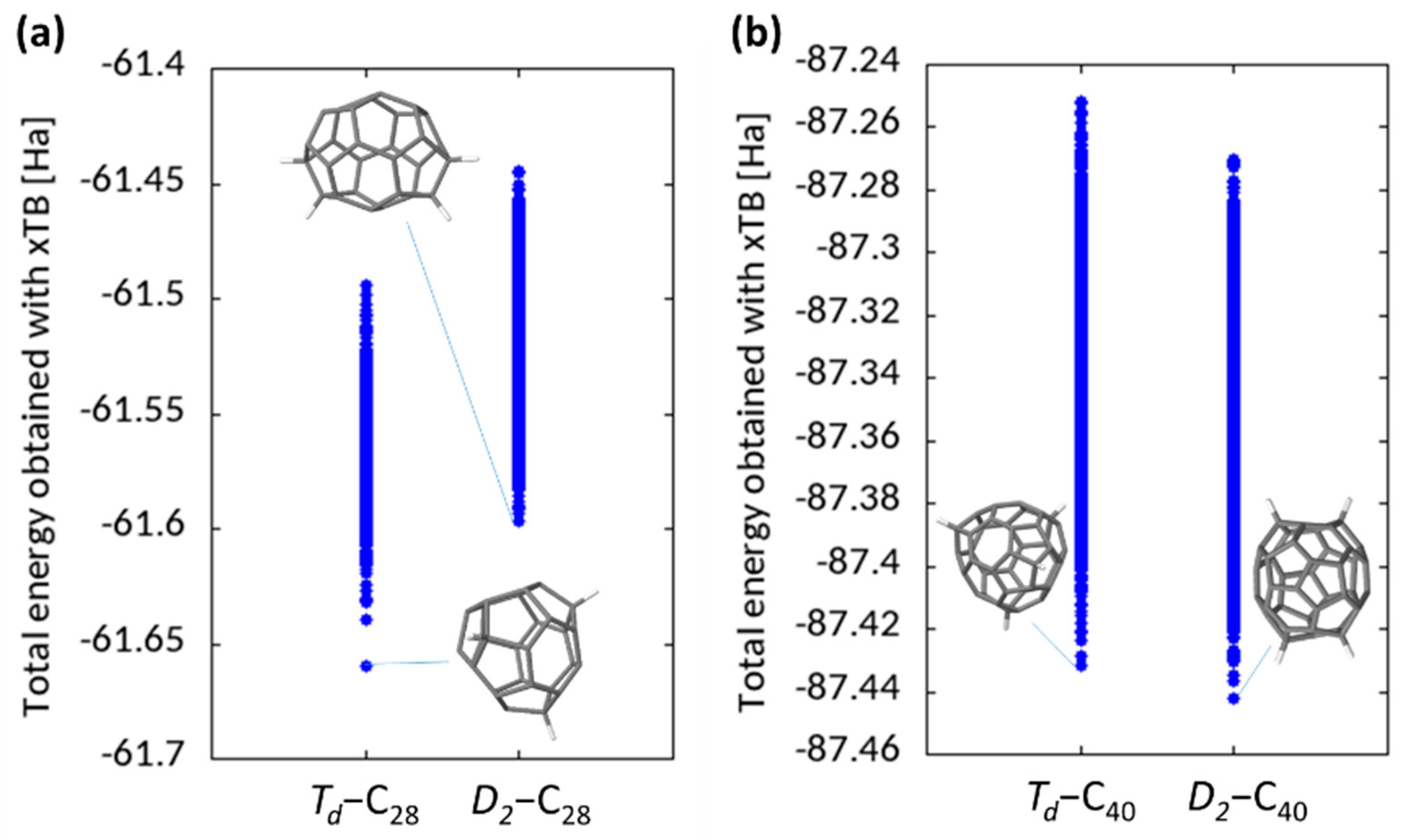
For C
28H
4, the most stable structure found is the
Td-C
28H
4 shown in
Figure 8 (Schlegel projection shown in
Figure S1). This has tetrahedral symmetry, and corresponds to the structure found in the literature [
23]. This is also the most stable structure found through sequential addition (using DFT-LDA, GFN2-xTB, PM7, PM6 + D3, and RM1). Energies of all the possible isomers are summarised in
Figure 8. The single data point at the lowest energy lies significantly below the others, i.e., for C
28H
4, there is a single stable hydrogenated structure. The
D2-C
28 isomer is significantly less stable; within the
D2-C
28H
4 subset of results, the most stable isomer consists of two hydrogen pairs at opposing ends of the molecule. This can be understood in terms of a localisation of strain, allowing a maximum flattening out and aromaticity in the two hexagon pairs along the fullerene sides. This structure is different, and more stable, than that found for
D2-C
28H
4 by sequential addition in
Section 3.2 above (confirmed with DFT-LDA to be more stable by 0.21 eV).
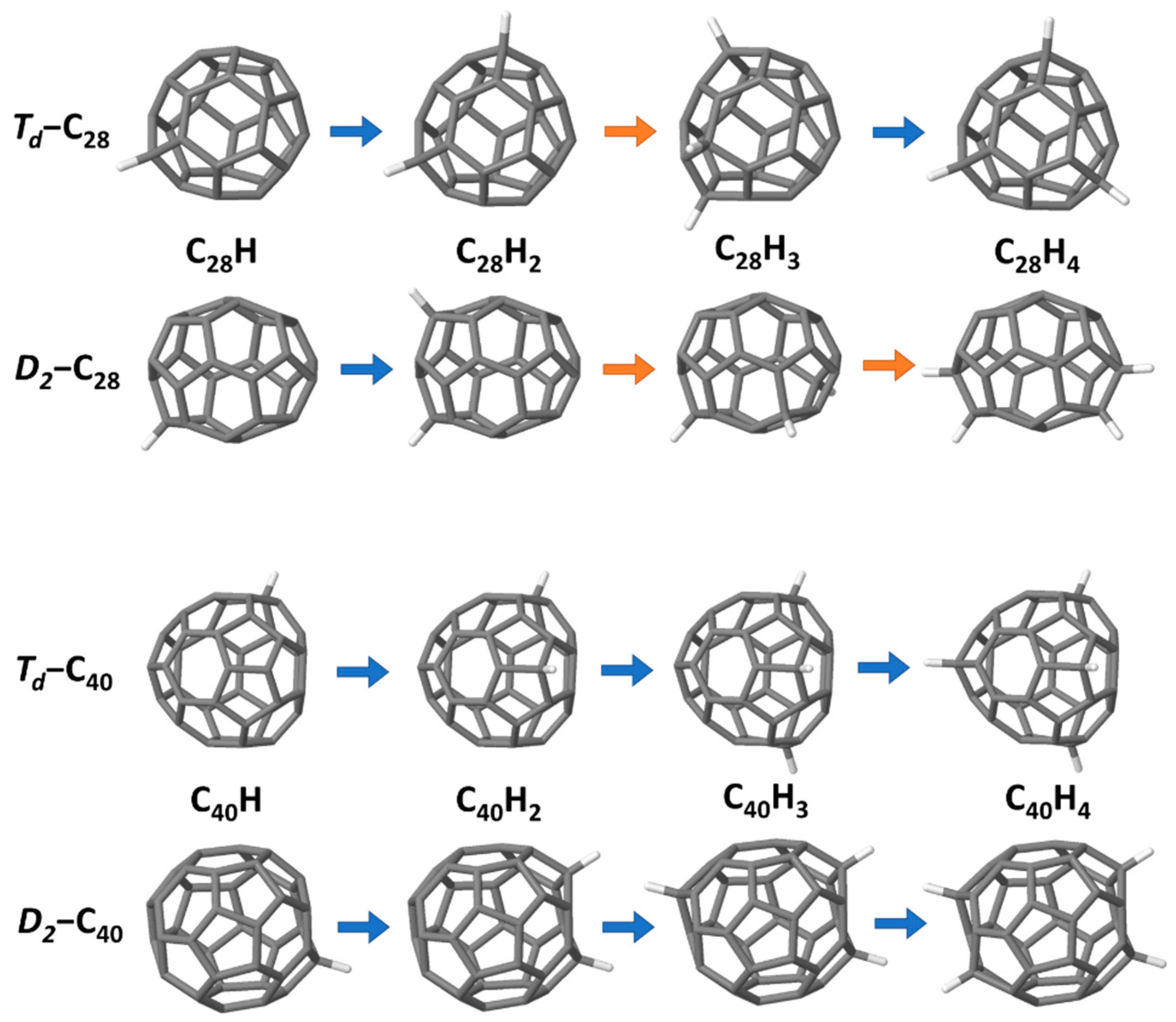
The lowest-energy C
nH
m structures for H = 1…4 for the two isomers are shown in
Figure 9. The
Td sequence for C
28 is largely sequential functionalisation of the triple pentagons, the exception being C
28H
3. In this case, the sequential structure has only a single unfunctionalised triple pentagon, which means the radical is highly localised, and hence, it is more stable to redistribute the hydrogen atoms. In contrast, the
D2-C
28 lowest-energy series is not at all sequential, with different hydrogenation combinations balancing the relief of localised curvature at the fullerene “ends” with radical redistribution. This flux of different structures is also presumably indicative of the relative instability of this isomer compared to the
Td.
The situation with C
40 is somewhat different. In this case, the most stable structures match exactly the series found through sequential addition in
Section 3.2. For the
Td-isomer, this is presumably because, in this case, the curvature at the triple pentagon is less localised than in C
28 due to the larger cage size, allowing more delocalisation of the radical for C
40H
3. For the
D2 isomer, hydrogenation localises the curvature at the fullerene ends, resulting in a cylindrical structure somewhat resembling a small-diameter capped carbon nanotube. The
D2 isomer is the most stable for all species up to C
40H
4. The relative energies show that hydrogenation is increasingly stabilising the
Td isomer (and indeed, as shown above, at C
40H
5, there is an inversion in stability and the
Td is more favoured). Further testing will be needed to determine whether, in larger fullerenes such as C
40 and above, the lowest-energy hydrogenated fullerenes always match the sequential addition patterns. If so, this would represent a significant computational benefit.
4. Discussion
This study draws out several key points when designing a methodology to explore the vast configurational space of hydrogenated isomers of small fullerenes.
The first is that, unfortunately, it does not appear possible to systematically predict subsequent lowest-energy hydrogenation sites based on either the geometry or electronic structure of a given fullerene or hydrogenated fullerene, at least not with the parameters that we have tested here. There are a number of potential reasons for this, including substantial strain relaxation of the structure, and charge and aromaticity redistribution after hydrogenation.
It has also been demonstrated that sequential hydrogen addition to the lowest-energy site at each step does not always result in the global lowest-energy hydrogenated fullerene isomer. Nonetheless, this procedure generates quite low-energy pathways and, in many cases, effectively did identify the lowest-energy isomers. It may be possible to use a modified version of this procedure (for example, allowing hydrogen atoms a limited number of site changes to neighbouring sites before subsequent hydrogen addition) in order to improve the robustness of the algorithm while maintaining a tractable number of structures to explore. Additionally, under laboratory hydrogenation conditions, where kinetic barriers for surface migration may be difficult to overcome, this hypothesis may still result in predicting experimentally detectable isomers, which may not necessarily be those with the lowest total energy.
Considering both the calculation costs and the correlation to full DFT-LDA results, GFN2-xTB appears to give reliable and rapid results for hydrogenation of small fullerenes. The predictability is supposed to originate with the DFT-based parameters for the electron density in the reference data.
Comparison with higher levels of theory highlights several points. First, the agreement between xTB and DFT-LDA found here will be fully reproduced with xTB and GGA functionals. Plotting LDA total energies against GGA, GGA-D2, and GGA-D3(BJ) energies for 741 hydrogenated fullerenes shows an R
2 value of ~1 (see
Supplementary Figure S4). This also validates a choice of either LDA or GGA-Dx for the energetics of these systems. When we compare against hybrid functionals (B3LYP using CAM-B3LYP with the Def2TZVP basis set and GD3BJ dispersion corrections [
68]) for the most and second-most stable isomers of
Td-C
28H
4 and
D2-C
28H
4, we find the same qualitative energy ordering, but a slight drop in the order of 0.1 eV in the absolute energy differences (see
Table S1 in Supplementary Materials). We have chosen to ignore thermal corrections to the energies in the current study as fullerene formation conditions in nonterrestrial environments are far from clear, as well as due to the high additional associated computational cost for vibrational analysis. Calculating thermal contributions with the hybrid functionals for these four fullerenes show that the thermal contribution to the relative stability between isomers is also of the order of ~0.1 eV, and again does not change the qualitative stability ordering of the isomers.
In the case of C28, the lowest-energy hydrogenated structure is Td-C28H4 with tetrahedral hydrogenation; each triple pentagon is hydrogenated. This relaxes the angle strain localised on the tetrahedral corners and is consistent with literature observations. For the D2-C28 isomer, there are two six-fused pentagons along its sides, and the curvature localised at the caps is partially relieved by pairwise hydrogenation at each cap. Nonetheless, the four hydrogen atoms appear insufficient to relax it and the structure is much less stable than the tetrahedral solution is.
In contrast, in the case of C
40, the
Td isomer is less stable than the
D2 isomer. Instead, the
D2 isomer, in which there are no triple-fused pentagons but two six-pentagon chains, shows the lowest energy. When we look at the structure of C
40H
4, fused pentagon (pentagon chains) sites are indeed hydrogenated [
3], not only on the triple pentagons. We suppose that for the larger fullerene cages, pentagon chain structures may play an important role to stabilise the whole structure of non-IPR species.
Given the rapidity and accuracy of the approach using GFN2-xTB, it is now our intention to pursue the most stable CnHm structures for other small fullerenes, with the eventual intention of mapping hydrogen-catalysed fullerene growth. For such large-scale studies, other methods beyond brute-force testing, such as genetic algorithms and Monte-Carlo-driven methods, will be required.


