Review

Application of Artificial Neural Networks in Crystal Growth of Electronic and Opto-Electronic Materials

1
Leibniz-Institut für Kristallzüchtung, Max-Born-Str. 2, 12489 Berlin, Germany
2
Leibniz Institute for Catalysis, Albert-Einstein-Str. 29A, 18069 Rostock, Germany
3
Institute of Computer Science, Pod Vodárenskou věží 2, 18207 Prague, Czech Republic
*
Author to whom correspondence should be addressed.
Crystals 2020, 10(8), 663; https://doi.org/10.3390/cryst10080663
Submission received: 31 May 2020 / Revised: 13 July 2020 / Accepted: 23 July 2020 / Published: 1 August 2020
(This article belongs to the Special Issue Crystal Growth from Liquid Phase)

Abstract

:
In this review, we summarize the results concerning the application of artificial neural networks (ANNs) in the crystal growth of electronic and opto-electronic materials. The main reason for using ANNs is to detect the patterns and relationships in non-linear static and dynamic data sets which are common in crystal growth processes, all in a real time. The fast forecasting is particularly important for the process control, since common numerical simulations are slow and in situ measurements of key process parameters are not feasible. This important machine learning approach thus makes it possible to determine optimized parameters for high-quality up-scaled crystals in real time.

1. Introduction

The crystal growth has a multi-disciplinary nature where heat, momentum and mass transport phenomena, chemical reactions (e.g., crystal and melt contamination) and electro-magnetic processes (e.g., induction and resistance heating, magnetic stirring, magnetic breaks, etc.) play a crucial role. Phase transformation, scaling problem (solid/liquid interface control on nm scale in growth system of ∼m size), numerous parameters (10 or more [1]) that have to be optimized, many constrains among them, and especially the dynamic character of the crystal grow process, make its development a difficult task.
The primary objective of this paper is to provide a comprehensive overview about the potential of artificial intelligence (AI) in crystal growth by addressing pros and cons of the AI technology for the enhancement of the growth of affordable high quality bulk crystals with higher aspect ratios.
Particular focus will be laid on the crystal growth of semiconductors, oxides and fluorides using Czochralski (Cz), vertical gradient freeze (VGF), directional solidification (DS) and top seeded solution growth (TSSG) methods.
The content of this paper is presented as follows: a general overview about the challenges in crystal growth and potentials of AI is given. In this context, increased emphasis will be placed ANNs as a large class of machine learning algorithms that attempt to simulate important parts of the functionality of biological neural networks. Machine learning is a subarea of AI that attempts to imitate with computer algorithms the way in which humans learn from previous experience.
This general overview is followed by introducing the reader to the basics of ANN modeling and other relevant statistical methods. The next section gives examples of already successful applications of ANN in the crystal growth. Finally, the main points and outlook of this highly industrially important technique are summarized.

2. Crystal Growth Challenges and AI Potential

The demand for low cost high quality bulk crystalline materials mainly for the electronic, photovoltaic and automotive industries increases at a very high rate in the recent decade [2]. The key challenge inherent in crystal growth is the fact that crystals are grown from melts at hostile process conditions with high crystal contamination risks and long processing times (i.e., on the very small spatio-temporal scales). Typically the growth processes last several days or a week and depend on many process parameters that have to be optimized.
Despite many crystals of semiconductors, oxides and fluorides have a number of unrivaled outstanding physical properties, their industrial production is limited by their low heat conductivity that hampers latent heat removal and lowers growth rates. As a consequence, a curvature of the crystallization front easily becomes concave, causing thermal stress within a crystal and an occurrence of dislocations. If the critical shear stress is low, high dislocation density under lower thermal stress will be induced, causing degradation of the crystal quality. A common approach to improve the process economy is to increase the crystal growth rate and to scale up the ingot size, i.e., to increase its diameter and its length. However, this is a difficult task.
In the past, the process development and optimization were based on general experiential learning that is rather speculative when applied at the industrial scale or for growing new materials. Nowadays, computational fluid dynamics (CFD) simulations combined with model experiments on a small scale and close-to-real experiments on pre-industrial scale have helped understanding the crucial process steps and factors determining the crystal growth [1]. A time-dependent CFD simulation of the real long running growth process is accurate, but slow, particularly in 3D. There are three major origin of errors in the CFD results: non-available or inaccurate material data, inadequate mesh and oversimplification of the CFD model. The origin of error in the material data may come from neglecting or not knowing their temperature dependence, anisotropy and/or their variable nature. The presence of poor-quality mesh elements (e.g., in crystal neck) may cause the ill-conditioned problem of stiffness matrix during the simulation, which could seriously affect the stability and convergence of a solver and the accuracy of the solution [3]. The last origin of errors is related to oversimplification of the furnace geometry (e.g., selection of a 2D model for non or partly axisymmetric geometry) and of selected physical models (e.g., neglecting turbulence or selecting non-appropriate turbulence model, transient behaviour, etc.).
Model experiments are usually based on the crystal growth of model substances [4] at low temperatures in small cylindrical crucibles. Alternatively, dummy solids are used at higher temperatures, but below their own melting point. Since model experiments are associated with severe simplifications: (i) the significant difference in material properties between model materials and growth materials, (ii) radiation is a dominant mode of heat transfer at high growth temperatures, but negligible near room temperature, (iii) rectangular geometry of the industrial equipment, and (iv) no convective heat and mass transport exist in the dummy solids, the higher scale-up ratios based on model experiments easily become speculative. The fundamental approach to scale-up is achieved by applying a principle of similarity which involves maintaining constant from a small scale to the commercial equipment the dimensionless groups (e.g., Reynolds, Grashof, Nusselt number, etc.) characterizing the phenomena of interest. However, in complex crystal processes, this is difficult, if not impossible, to attain. Nevertheless, the similitude analysis, even incomplete, enables one to identify the most important growth determining steps.
Pre-industrial scale crystal growth experiments with industrial feedstock and corresponding CFD simulations significantly improve the accuracy of the technology development for the industrial applications, but seriously increase the developing time and costs for the new technology. Moreover, crystal growth technology still strongly depends on labor skills/human ability that are always subject to errors.
In consequence, it took, e.g., ca. 40 years to enlarge Si wafers diameter from 1 inch to 12 inch.
Artificial intelligence has been recently considered as the fundamental tool for obtaining knowledge and analyzing cause-effect relationships in complex systems in a big-data environment, particularly for the optimization of process parameters and automation of manufacturing. Despite tremendous success in many fields of science and industry, including solid state material science and chemistry [5,6], wider applications in the crystal growth are still missing. The main reason lays in the fact that the ultimate success of AI is usually linked with so-called 4V challenges: data volume, variety, veracity and velocity. In the experimental crystal growth, large datasets are seldom available, the range of useful process parameters is rather narrow and the data trustworthiness is an issue. The data veracity is a challenge, since in situ in operando measurements of important process parameters are constrained by the aggressive environment and high purity requirements. In the industry, the apparent volume of data is high; however, due to the ageing of the equipment and often small changes in the growth recipe and/or hot zone parts, the data veracity is questionable.
Recently, many different approaches were proposed in the literature how to tackle the 4V constrains, e.g., to use CFD simulations to generate large and diverse datasets in combination with available experimental data for validation. On the other hand, the volume of the needed training data can be reduced by using advanced machine learning methods known as active learning and transfer learning [7]. Various examples of the successful ANN applications will be presented in Section 4.

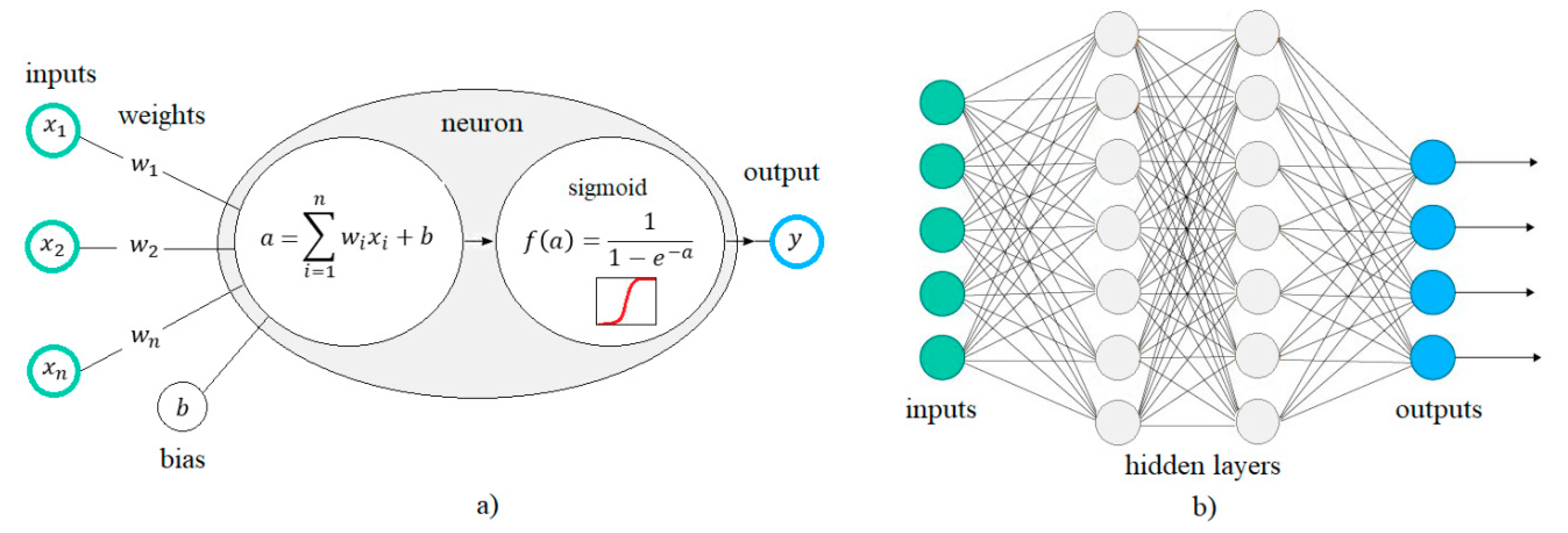
3. Artificial Neural Networks Overview

Machine learning is an area in computer science aiming to optimize the performance of a certain task throughout learning from examples and/or past experience. Neural networks are by far the most widespread technique of machine learning. There are many kinds of neural networks, differing most apparently through the architecture connecting their functional units−Neurons (Figure 1), each with their unique strengths that determine their applications. The most important neural network types for materials science/crystal growth will be a topic of this chapter.
The Artificial Neural Network (ANN) is a statistical method inspired by biological processes in the human brain able to detect the patterns and relationships in data. ANNs are particularly powerful in correlating very high number of variables and for highly non-linear dependences [8].
An ANN is characterized primarily by its architecture, i.e., a set of artificial neurons and connection patterns between them. The neurons are often organized into layers: an input layer, hidden (intermediate) layers and an output layer (Figure 2). Each neuron acts as a computational unit. It receives inputs x i , and multiplies them by weights w i (a synaptic operation) and then uses the sum of such weighted inputs as the argument for a nonlinear function (somatic operation), which yields the final output of the neuron y j (known as neuron activation). The whole ANN receives inputs by neurons in the first layer, and provides output by the neurons in the last layer.
The most common activation function has been taken over from the logistic regression, well known in statistics, which is why it is called logistic sigmoidal function f(x,w) (1):
y j = f ( x , w ) = 1 1 + e ( i = 1 n ( w j , i x i + b i ) )
By adjusting the weights w j , i of connections and biases b i of artificial neurons (process known as ANN training), one can obtain the targeted output y j for a specific combination of inputs x i . The final goal of ANN training is to adjust the weights and biases to minimize some kind of error E measured on the network.
For crystal growth, the most relevant kind of error is the sum of squared differences between the outputs y j of the network and the desired output o j , summed over all the neurons in the output layer (2):
E ( x , w , o ) = j ( y j o j ) 2
The weights can be, in the simplest case, adjusted using the method of gradient descendent [9] with constant learning rate η (3):
Δ w j , i = η E w j , i
Prior to ANN training, it is necessary to select its architecture, the activation function and training method.
A suitability of different ANN architectures is most reliably compared by the k-fold cross validation method [11]. First, the training set is partitioned into k subsets. For each architecture, the training is performed k times, each time using one of the subsets as the validation set and the remaining subsets as the training set. In the next step, the architecture that had the smallest error averaged over the validation sets from the k runs is selected. Finally, the network with that architecture is used to train with all of the data. In traditional feed-forward neural networks with one or only few hidden layers (so called shallow networks), three training algorithms are most frequently used: Levenberg–Marquardt, Bayesian regularization and Scaled conjugate gradients [10]. After being trained, the ANN model reflects the relationship between the input and output of the system.
If an ANN is expected to correlate variables evolving in time, a dynamic ANN should be used [12]. The forecasting of time series is a typical problem in process control applications [13]. The response of a dynamic ANN at any given time depends not only on the current input, but on the history of the input sequence. Consequently, dynamic networks have memory and can be trained to learn transient patterns. Temporal information can be included through a set of time delays between different inputs, so that the data corresponds to different points in time. There are several types of dynamic ANN models that can be used for time-series forecasting: e.g., Long Short-Term Memory (LSTM), Layer-Recurrent Network (LRN), Focused Time-Delay Neural Network (FTDNN), the Elman Network, and Networks with Exogenous Inputs (NARX) [14,15].
NARX are time-delay recurrent networks suitable for short time lag tasks. They have several hidden layers that relate the current value of the output to: (i) past values of the same variable and (ii) current and past values of the input (exogenous) variables (Figure 3). Such a model can be described algebraically by Equation (4):
y [ t ] = f ( x [ t d x ] , , x [ t 1 ] , x [ t ] , y [ t d y ] , , y [ t 1 ] , θ )
where y[t] ∈ RNy is an output variable, x[t] ∈ RNx an exogenous input variable, f is a non-linear activation function (e.g., sigmoid),   θ is an error function, dx and dy are input and output time delays.
The input i[t] of the NARX network has dxNx + dyNy components:
i [ t ] = [ ( x [ t d x ] , , x [ t 1 ] ) T ( y [ t d y ] , , y [ t 1 ] ) T ] T
In the equation, T is a notation for the transpose of a matrix. The output y[t] of the network is governed by the Equations (6)–(8):
h 1 [ t ] = f ( i [ t ] , θ 1 ) ,       θ 1 = { W i h 1 R ( d x N x + d y N y ) × N 1 , b h 1 R N 1 }
h l [ t ] = f ( h l 1 [ t 1 ] , θ l ) ,           θ l = { W l l R N l 1 × N l , b l R N l }
y [ t ] = g ( h N l [ t 1 ] , θ 0 ) ,       θ 0 = { W h N l 0 R N N l × N y , b 0 R N y }
where h1 [t] ∈ RN1 is the output of the input layer at time t , h l [ t ] R N l is the output of the l-th hidden layer at time t, g(·) is a linear function, θ1 are the parameters that determine the weights in the input layer, θl in the l-th hidden layer and θ0 in the output layer.
NARX networks are trained and cross validated in the same way as the static ANNs.
For solving complex long time lag tasks, LSTM networks are a better choice. LSTM network was proposed in [16] as a solution to the vanishing gradient problem found in training ANNs with gradient-based learning methods and back-propagation, where the training process may completely stop, i.e., weights do not adjust their values anymore. An LSTM uses a broader spectrum of information than more traditional recurrent networks. To this end, it consists of gated cells that can forget or pass on information, based on filters with their own sets of weights, as usually adjusted via network learning. By maintaining a more constant error, LSTM can learn over many time steps and link distant occurrences to a final output.
A Convolutional neural Network (CNN) is a special type of a neural network mostly used for image and pattern recognition. A CNN consists of multiple, repeating components that are stacked in basic layers: convolution, pooling, fully connected and dropout layer, etc., similar to most other types of ANNs (Figure 4) [17]. A convolution layer applies a convolution filter to its input data. A pooling layer maximizes or averages values in each sub-region of the feature maps. A fully connected layer connects one neuron in the next layer to each neuron in the previous layer by a weight, like in the traditional feed-forward networks described earlier in this chapter. Activation functions as part of the convolutional layer and the fully connected layer are used to introduce nonlinear transformations into the CNN model. A dropout layer randomly ignores (drops out) a certain number or proportion of neurons and therewith decreases the danger of overtraining (and also training costs).
In the literature, most of the studies on the application of ANNs in the crystal growth were devoted to optimization problems. Fortunately, optima of ANNs can be determined applying methods for differentiable functions on ANN (almost all ANNs can be differentiated). Another optimization method sometimes encountered in this context, are Genetic Algorithms (GAs). Due to their popularity in various scientific fields in or adjacent to the material science [5,18,19], they will be shortly described.
A GA is the probably best known representative of evolutionary algorithms, which are stochastic methods for solving optimization problems based on the idea of biological evolution and natural selection. A GA repeatedly modifies a population of individual solutions, by randomly selecting individuals from the current population, evaluating and ranking them according to their fitness value and then either forwarding them to the next generation if they belong among those with the best fitness value, or recombining them or mutating them to produce the children for the next generation. Over consecutive generations, the population will evolve to better and better solutions (Figure 5).
A probability p S ( X i ) that the individual X i   in the population of N individuals will be selected to become a parent depends on its fitness value f ( X i )   that first has to be normalized according to Equation (9):
p S ( X i ) = f ( X i ) j = 1 N f ( X i ) ,       i = 1 , 2 , , N
For the proportional selection scheme (roulette wheel), X i   will be selected if a random number ξ with uniform distribution on the interval [0,1] satisfies Equation (10):
j = 0 i 1 p S ( X j ) < ξ < j = 0 i p S ( X j ) ,     p S ( X j ) = 0     for   j = 0
Two individuals described with vectors of real numbers X , Y that are selected as parents will recombine with probability p c , producing the new individuals   X , Y according to Equation (11):
{ X = ξ X + ( 1 ξ ) Y , Y = ξ Y + ( 1 ξ ) X ,
where ξ is a random number with uniform distribution on the interval [0,1].
Mutation of the individual X will produce in the next generation with probability p m an individual X according to Equation (12):
X = ξ + X
where ξ is a random vector with Gaussian distribution with zero mean and unit variance.
When combining an ANN and a GA, a search for the optimum starts by randomly generating a set of inputs and their corresponding outputs predicted by ANN. Candidate solutions are then selected according to their fit to previously defined criteria; the GA is then used for evolving new solutions to the problem using crossover and mutation. This is repeated until the optimization criteria are fulfilled [20].
An inherent stochastic nature of the crystal growth data originates from, e.g., inaccurate measurements or inaccurate simulations of the crystal growth process parameter: crucible rotational rate, crystal rotational rate, crystal pulling rate, gas pressure, gas flow rate, heating power, melt loading, etc. Addressing the uncertainty of ANN predictions is feasible if on ANN is superimposed a Gaussian process model (GP) [21]. Due to a high potential benefit for crystal growth applications, this combined ANN and GP approach will be shortly described.
GP is a statistical method capable of modeling the probability distribution of output values Y x for arbitrary sets of inputs x 1 , , x n simultaneously [21]. A simple example of GP in one dimension is illustrated in Figure 6.
Mathematically speaking, a GP is a collection ( Y x ) x k of random variables Y x assigned to points from a k -dimensional vector space k and such that any finite subcollection corresponding to some n points x 1 , , x n from that space has a multivariate Gaussian distribution:
( Y x 1 , , Y x n ) ~ N ( μ ( x 1 , , , x n ) , Σ ( x 1 , , x n ) )
Here, μ is a the GP mean, determined by a function that models the non-stochastic part of the data, and the covariance matrix Σ ( x 1 , , x n ) is determined by a symmetric function K : k × k , called covariance function, on which usually a Gaussian noise with a variance σ G 2 is superimposed:
( Σ ( x 1 , , x n ) ) i , j = K ( x i , x j ) + σ G 2 I n , i , j = 1 , , n ,
where I n denotes the n -dimensional identity matrix. One possible covariance function is defined in (15),
K ( x i , x j ) = σ f 2 exp ( x i x j 2 2 σ l 2 )
where σ f 2   and σ l 2 are GP hyperparameters, i.e., signal variance and the characteristic length scale of Gaussians in the space   k , respectively. The hyperparameters and the Gaussian noise dispersion σ G 2 are usually estimated with the maximum likelihood method, i.e., through maximizing the density (13) of ( Y x 1 , , Y x n ) corresponding to the vector ( y 1 , , y n ) from a given training set ( ( x 1 , y 1 ) , , ( x n , y n ) ) . Once the hyperparameters have been estimated, allowing to compute the value K ( x , X ) for any   x , X ϵ k , (13) and (14) can be used to predict the distribution of Y x for any x x 1 , , x n . This yields:
Y x ~ N ( μ ( x ) + ( K ( x , x 1 ) , , K ( x , x n ) ) Σ ( x 1 , , x n ) 1 ( y 1 , , y n ) , Σ ^ x )
where Σ ^ x = K ( x , x ) + ( K ( x , x 1 ) , , K ( x , x n ) ) Σ ( x 1 , , x n ) 1 ( K ( x , x 1 ) , , K ( x , x n ) ) .
When combining ANN and GP, i.e., if trained ANN is used as the GP mean function (Equation (13)), more information will be obtained about the system than from one single method. ANN offers information about the functional dependence among the variables and GP about the random influences.

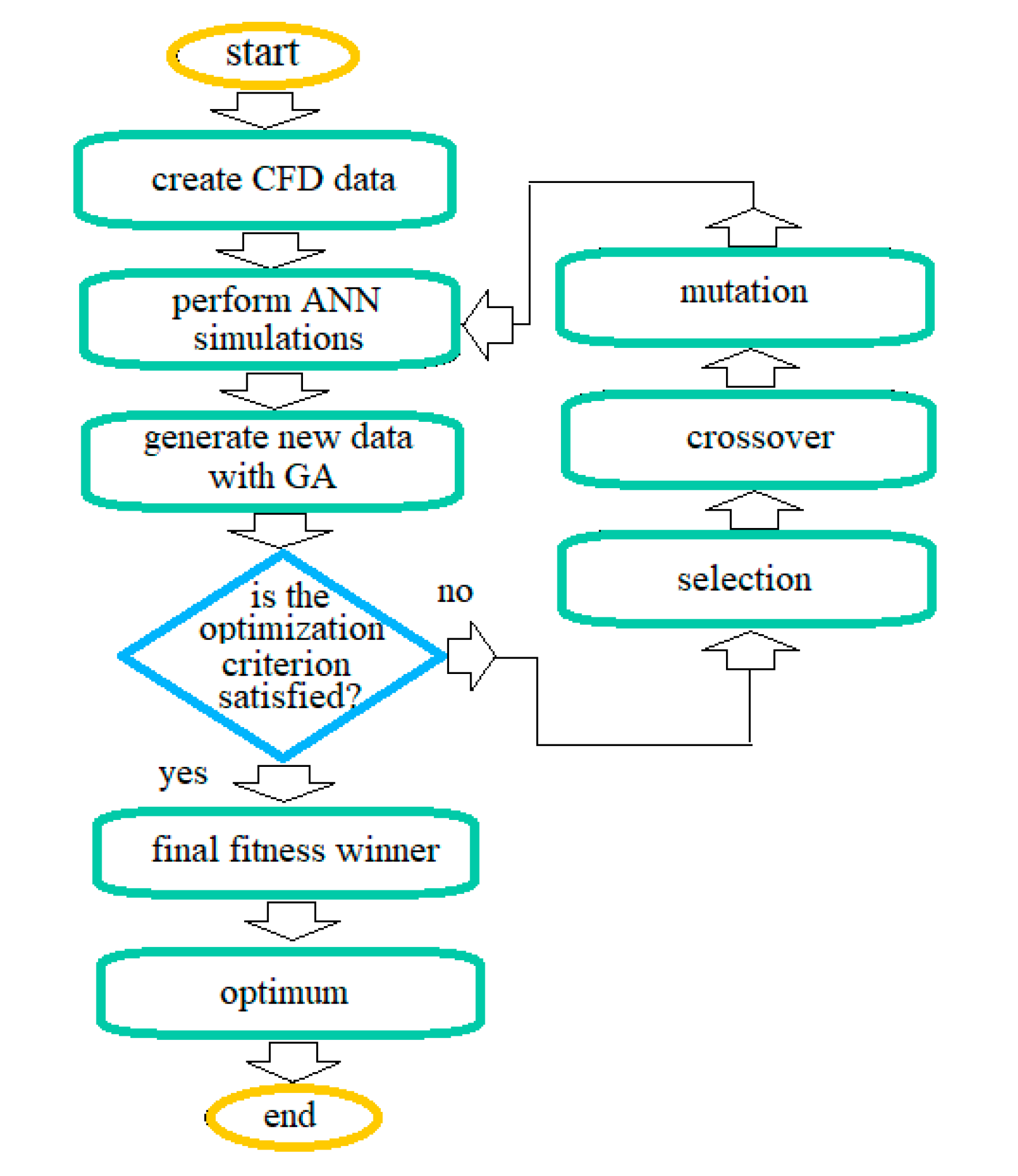
4. AI Applications in Crystal Growth: State of the Art

The application of ANNs in the crystal growth received much attention in the last decade. Still the studies are rare [18,23,24,25,26,27,28,29,30,31,32,33,34,35,36,37]. Only part of them were devoted to the crystal growth of semiconductors and oxides [18,26,27,28,29,30,31,32,33,36,37]. Up to now, there have been two main research topics: optimization of the crystal growth process parameters and crystal growth process control by static and dynamic ANNs, respectively.

4.1. Static ANN Applications

Concerning static applications, in the papers [25,26,29,31], feed-forward networks of either the mono- or multi-layer perceptron type were used to model dependences pertaining to crystal growth process.
In [26], TSSG of SiC crystals for power devices was studied. To make high-quality large-diameter (8 inch) SiC crystals using the TSSG method able to compete commercially standard SiC crystals grown by sublimation method, it is necessary to optimize the spatial distribution of supersaturation and the flow velocity in the solution (Figure 7a). In the literature, it was reported that solution flow from the center to the periphery gave rise to a smooth surface on the crystal [38]. The beneficial supersaturation distribution is the one in which the supersaturation near the seed crystal is relatively high and the supersaturation near the crucible bottom and wall is low. The TSSG optimization is a challenging task since the velocity and supersaturation depend on many process parameters (e.g., heater power, crucible position and rotation, seed crystal position and rotation, growth configuration of the heat insulator, crucible shape, and crucible size) that must be optimized simultaneously. Moreover, these parameters need to be optimized with respect to multiple objectives.
Common experimental and CFD approaches to the optimization of the process parameters are laborious and time consuming. The authors of [26] proposed the application of ANN for acceleration of CFD simulations, combined with GA for the process optimization. The database for the ANN training was derived from CFD simulations. Resulting feed-forward ANN with 4 hidden layers was derived from 1000 steady axisymmetric CFD simulated process recipes, able to correlate 11 inputs (boundary temperatures, seed rotation rates, sizes of the crucible and seed and spatial coordinates (r,z) of 400 points in the axisymmetric computational domain) with 3 outputs (flow velocity components (radial ur, axial uz) and chemical composition of the solution in the points in the computational domain shown in Figure 7b. The comparison of the ANN and CFD predictions of the flow and concentration patterns are shown in Figure 7c. The ANN predictions mimicked the CFD results and were 107 times faster than the corresponding CFD simulations, enabling also fast optimization of the process parameters in the large parameter space. The superposition of the GA to the ANN prediction model enabled more optimum conditions to be found. The prediction of the growth conditions for upscaled SiC crystals using the same methodology was the topic of the authors’ further papers [32,33].
Concerning the proposed method of CFD acceleration by ANN for optimization purposes, the question is often raised whether it is worth training ANN using thousands of CFD simulations or it is more efficient way to increase the computational power to perform solely the CFD simulations of the required case? The answer may lay in the economics of scale. The number of CFD cases that one has to run is exactly proportional to the processing power, while the number of cases that one avoids running because one has a trained ANN can by many orders of magnitude exceed that. Therefore, the more parameters to optimize, the better is the economy of ANN method for high speed predictions of CFD results. Nevertheless, the strength of ANNs in CFD modelling is more in model deduction, not in replacing the solver itself.
More researchers studied the application of static ANN combined with GA [18,31] or the Adam optimization method [39] for the optimization of parameters affecting the crystal growth [26].
For example, the prediction and optimization of parameters affecting the temperature field in the Czochralski growth of YAG crystals using data based on axisymmetric steady state CFD simulations was studied in [18]. In the Czochralski crystal growth process, a flat crystallization front during the growth assures production of single crystals with less structural defects, uniform physical properties and homogenous chemical composition. The study was focused on the influence of the crystal pulling rate, crystal rotational rate, ambient gas temperature and temperature of crucible on the deflection and the position of the crystallization front. The ANN with 4 inputs, 1 hidden layer and 2 outputs, derived from only 81 simulations was used. The CFD results were verified with Cz-InP growth experiments published in [40] (Figure 8b). Moderate accuracy of the ANN predictions may originate either from simple architecture of the ANN and low number of training data or from inaccurate CFD results used for ANN training. The latter may be an issue due to the over simplified CFD model (e.g., simple boundary conditions and steady state assumption) and verification of the obtained results using the crystal growth experiments for another material. This example of the ANN application revealed the greatest drawback of the usage of ANNs if based on CFD data. ANN strongly rely on the training data veracity. It can only extract information which is present in the input and map it into its training set, but ANN cannot compensate the inaccuracy of the CFD results in cases of a lack of experimental validation of the data.
Another example of the application of static ANN for optimization tasks is described in [37]. The authors addressed the common problem of accurate monitoring of temperatures during the directional solidification of silicon (DS-Si) with limited number of thermocouples. They used 195 data sets generated by 2D CFD modeling to train ANN with 8 inputs (3 temperatures of heaters, 4 equidistant temperatures along the crucible side wall and 1 crucible axial position) and 21 outputs (21 equidistant temperatures along the crucible side wall). The best predictions were obtained for the architecture with 2 hidden layers with 32 neurons. The top ten ranks of accurate temperature predictions contain positions around the crucible bottom, suggesting the importance of measuring temperatures in the zone of high-temperature gradients. This approach and the obtained results may be of interest for the prediction of the location and a reduction in the number of thermocouples inside small crystal growth furnaces. Nevertheless, the accuracy of the ANN predictions will again strongly depend on the accuracy of the CFD results, particularly for the processes such as DS-Si, when an axisymmetric CFD model is used for the description of the rectangular set-up. For these cases, prior to ANN training, the verification of the CFD model with crystal growth experiments is indispensable.
Feasible approach for the ANN applications with inaccurate input values or more than one possible solution is to provide uncertainty information to the ANN predictions by the superposition of ANN with a GP. This combination of two statistical methods was used in [29,30] for a fast prediction and optimization of magnetic parameters for temperature field management, i.e., for flat solid–liquid interface deflection Δ (|Δ| < 0.1 mm), in magnetically driven DS-Si and VGF of GaAs. In [29], 4 inputs (frequency, phase shift, electric current amplitude and crystal growth rate) were correlated with 1 output (solid–liquid interface deflection Δ in magnetic field) using mono layer feed-forward ANN based on 437 CFD axisymmetric quasi steady state simulations, verified with available experimental results (Figure 9). Finally, ANNs were combined with GP models to derive the probability distribution of the output for every given combination of inputs (Figure 9c).
Analyzing the GP results shown in Figure 9c, it can be noticed the uneven narrowness in the spatial probability distribution. From the way how a GP was constructed follows that the uncertainty of the GP predictions depends on local data density, i.e., if there is a high density of training data, variance of the predicted Gaussian distribution is small, while for outliers or in sparsely populated regions of input space, it has a large variance. In view of this, a combination of ANN and GP offers more information than one single model, i.e., ANN offers information about the functional dependence and GP about the random influences.

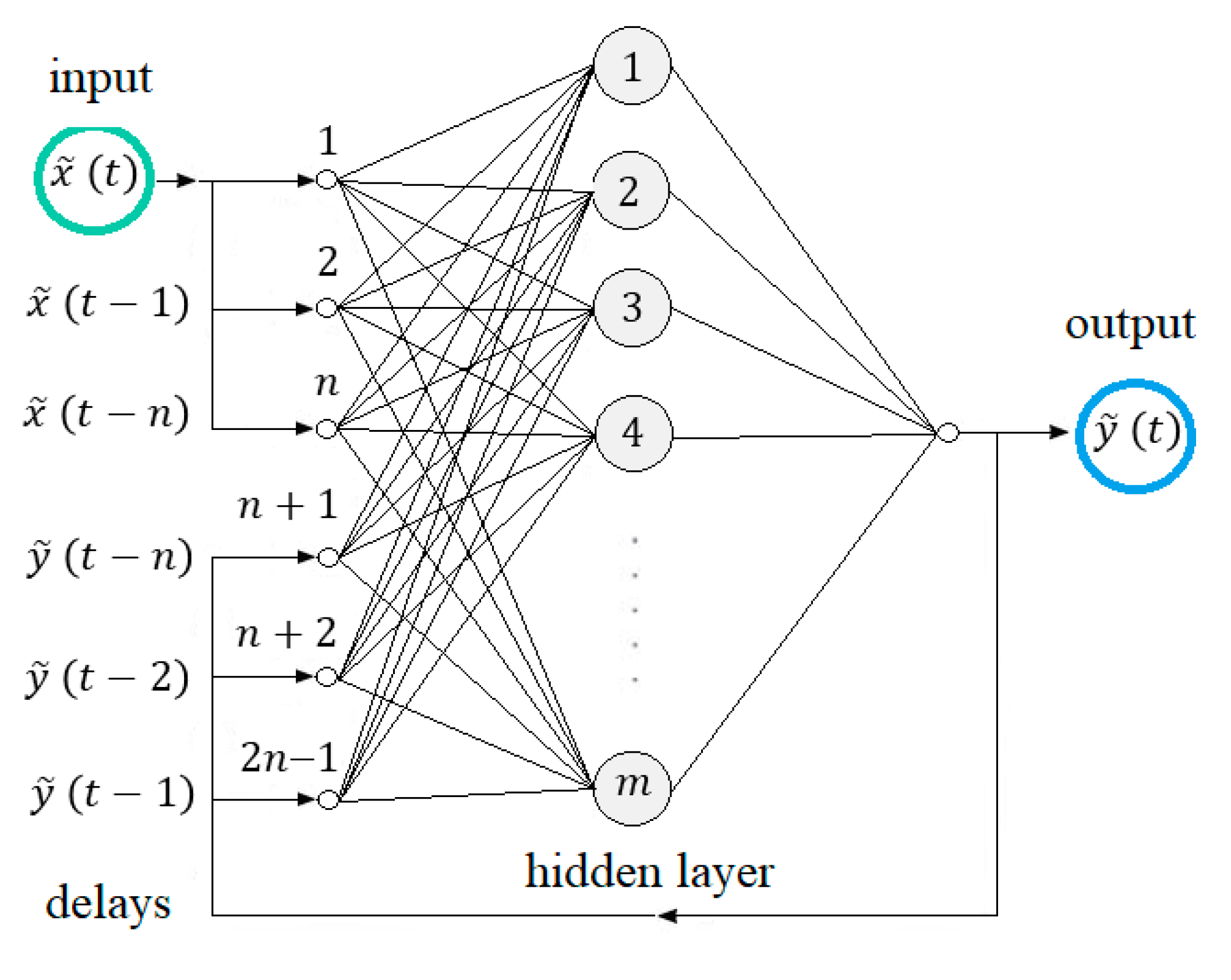
4.2. Dynamic Applications

Exact control of the dynamic processes at the crystallization front is a key for enhanced crystal growth yield and improved crystal quality. It is particularly important to suppress the turbulent motions in the melt and to control temperature gradients in the crystal that are responsible for the generation of detrimental crystal defects and undesired variation of crystal diameter. The complex solidification process is difficult to control due to the large time delays, high-order dynamics and constrains in using suitable sensors in the crystallization furnace because of the hostile environment.
The multivariable nonlinear model predictive control based on dynamic artificial neural networks is the most promising, real-time capable and accurate alternative to the conventional slow controllers based on linear theory.
The crystal growth process dynamics described by static feed-forward ANN was the topic of a paper [31]. In this study, 54 transient axisymmetric 2D CFD simulations were used to derive the cooling rates of two heaters and the velocity of the heat gate during directional solidification of 850 kg quasimono Si crystals in industrial G6 size furnace. These rates were correlated with crystal quality (i.e., thermal stress in crystal and solid/liquid interface deflection) and growth time using static ANN with 3 inputs, 1 hidden layer and 3 outputs (Figure 10). The growth recipe for the solidification step was optimized using GA. The total fitness of the evaluation was defined in Equation (17).
E t o t a l = 0.2 E d e f l e c t i o n + 0.6 E s t r e s s + 0.2 E t i m e
Fitness weights in Equation (17) were selected in cooperation with the industry where thermal stress is the most important factor to cause dislocations in crystal and therefore was assigned the highest weight value. Compared with the original crystal growth recipe, the optimized recipe has faster movement of the heat gate and larger cooling rate of the top heater, but smaller cooling rate of the side heater. Moreover, the cooling rates of both heaters in the optimal recipe decrease slightly with time. The authors found out that the optimization of the process for coupled ANN with GA is about 45 times faster than in the case of optimization with CFD. The proposed combination of transient CFD results for database and static ANN has both advantages and disadvantages. Typically, static ANNs are defined by less parameters (weights and biases) than dynamic ANNs, i.e., they require smaller number of datasets to assure identifiability of the parameters and they will be trained faster.
The drawback is the use of heating rates as static ANN inputs, since they are not experimentally measurable during the crystal growth process. Typical crystal growth furnaces use either power or temperature control of heaters. Therefore, this approach is not suitable for process control and automation. Moreover, the proposed methodology aims to find the optimum of ANN, not the optimum of the crystal growth problem.
Another concept for coping with process dynamics was proposed in a proof-of-concept study [28], where transient 1D CFD results of the simplified VGF-GaAs model provided the transient datasets of 2 heating powers and 5 temperatures at different axial positions in the melt and crystal and position of solid/liquid interface. Altogether 500 datasets were used for training a NARX type of dynamic ANN. The best results were obtained for NARX architecture with 2 inputs, 2 hidden layers with 9 and 8 neurons, 6 outputs, and 2 time delays (Figure 11b). The predictions were accurate for the slow growth rates (Figure 11c), but their accuracy decreased with the increase in the crystal growth rate. Beside a need for improved accuracy, for the practical application in process automation and control, it will be necessary to derive datasets from axisymmetric CFD simulations.
One more example of the application of dynamic ANN in the crystal growth of semiconducting films was presented in [36]. By Metal Organic Chemical Vapor Deposition (MOCVD) growth of GaN for microelectronic and optoelectronic devices, accurate temperature control is needed to maintain wavelength uniformity, control wafer bow and reduce wafer slip. It was reported on the development of a dynamic NARX ANN for a prediction of time series of 2 temperatures (2 outputs) given a time series of 2 heater filament currents, carrier rotational rate and operating pressure (4 inputs). The time series predictions served as a plant model in model predictive control. Very accurate predictions of temperatures with error ~1 K were obtained for the NARX architecture with 1 hidden layer of 10 neurons and 2 delays.
Different accuracy of the NARX predictions in bulk and films crystal growth in the above mentioned examples may be related to the different time scales of the transport phenomena (e.g., large time scale for the removal of the latent heat from the crystallization front in large industrial size bulk crystals versus short time scale in thin films) between these two crystal growth processes. NARX neural networks have shown success for many time-series modeling tasks, particularly in the control applications, but learning long-term dependencies from data remains difficult. This is often attributed to their vanishing gradient problem. More recent Long Short-Term Memory (LSTM) networks attempt to remedy this problem by preserving the error, which is then always back-propagated through time and layers [16]. By maintaining a more constant error, LSTM allows recurrent nets to continue to learn over many time steps. LSTM applications in the bulk crystal growth are still to come.

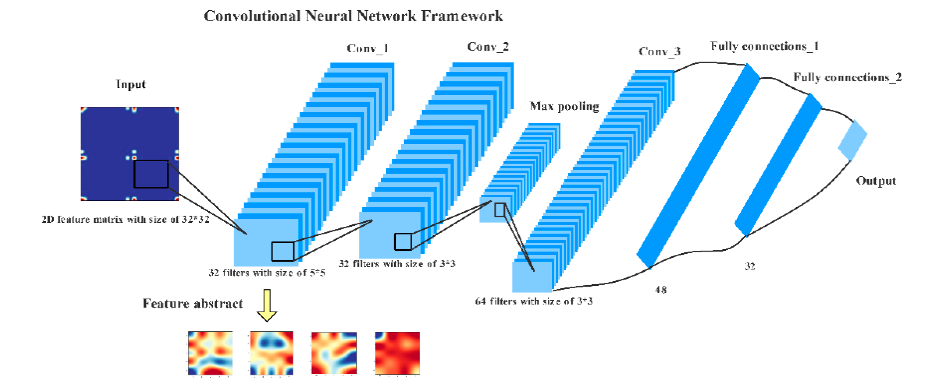
4.3. Image Processing Applications

Applications of CNN in the crystal growth are yet to come. Still, numerous papers are available on the applications of the CNNs in the fields pertinent to crystal growth simulations and crystal characterization, e.g., the prediction of turbulence [41], derivation of material data [5,42,43,44,45,46], optimization of CFD meshes [3], classification of atomically resolved Scanning Transmission Electron Microscopy (STEM) [47], and Transmission Electron Microscopy (TEM) [48] images, just to mention a few.

5. Conclusions and Outlook

The recent boom in ANN applications in various fields of science and technology was possible thanks to increased data volumes, advanced algorithms, and improvements in computing power and storage.
For the years to come, it is feasible to expect that novel ANN applications will significantly accelerate fundamental and applied crystal growth research. The gain in terms of scientific research lies in the fast and accurate ANN predictive power that is a stepping stone towards an explanation for new crystal growth theories and hypothesis, if a convincing theory is unavailable. ANNs predictive power enables/provides: (1) pre-selection of well performing scientific models for further studies, (2) quantitate comparison of scientific models on the base of their prediction success that might reveal factors relevant for their success and thus contribute to the theory development and (3) ultimate reliable criterion for successful explanation of new theoretical models, free from error-prone human judgement. Concerning crystal growth applications, the need for affordable high quality crystals of semiconductors and oxides is continuously increasing, particularly for the electronic and photovoltaic industries, i.e., for solar cells, electric and fuel cell vehicles. Fast optimization of the process parameters and their exact control is a key for enhanced crystal growth yield and improved crystal quality. The next generation of smart crystal growth factories will use AI and automation to keep costs low and profits high.
In this paper, we reviewed the recent ANN applications and discussed their advantages and drawbacks. The latest international activities have been devoted to the development of sustainable infrastructure for the provision of experimental, theoretical, and computational research data in the field of condensed-matter physics and materials science. Once available, the usage of open source big crystal growth data will resolve the last bottleneck for ANN applications and will strongly push the development of new breakthrough crystalline material-based technologies. Until then, the volume of required training data may be reduced by using advanced machine learning methods known as active learning [49,50,51,52,53].

Funding

The research reported in this paper has been partially supported by the Czech Science Foundation (GACR) grant 18-18080S.

Conflicts of Interest

The authors declare no conflict of interest.

References

  1. Scheel, H.J. The Development of Crystal Growth Technology. In Crystal Growth Technology; Scheel, H.J., Fukuda, T., Eds.; John Wiley & Sons, Ltd.: Hoboken, NJ, USA, 2003. [Google Scholar]
  2. Capper, P. Bulk Crystal Growth—Methods and Materials. In Springer Handbook of Electronic and Photonic Materials; Springer Science and Business Media LLC: Berlin/Heidelberg, Germany, 2006. [Google Scholar]
  3. Chen, X.; Liu, J.; Pang, Y.; Chen, J.; Chi, L.; Gong, C. Developing a new mesh quality evaluation method based on convolutional neural network. Eng. Appl. Comput. Fluid Mech. 2020, 14, 391–400. [Google Scholar] [CrossRef]
  4. Duffar, T. Crystal Growth Processes Based on Capillarity: Czochralski, Floating Zone, Shaping and Crucible Techniques; John Wiley & Sons: Hoboken, NJ, USA, 2010. [Google Scholar]
  5. Schmidt, J.; Marques, M.R.G.; Botti, S.; Marques, M.A.L. Recent advances and applications of machine learning in solid-state materials science. npj Comput. Mater. 2019, 5. [Google Scholar] [CrossRef]
  6. Butler, K.T.; Davies, D.W.; Cartwright, H.; Isayev, O.; Walsh, A. Machine learning for molecular and materials science. Nature 2018, 559, 547–555. [Google Scholar] [CrossRef] [PubMed]
  7. Smith, J.S.; Nebgen, B.T.; Zubatyuk, R.; Lubbers, N.; Devereux, C.; Barros, K.; Tretiak, S.; Isayev, O.; Roitberg, A. Outsmarting Quantum Chemistry through Transfer Learning. ChemRxiv 2018. [Google Scholar]
  8. Rojas, R. Neural Networks: A Systematic Introduction; Springer: Berlin, Germany, 1996. [Google Scholar]
  9. Hagan, M.T.; Demuth, H.B.; Beale, M.H. Neural Network Design; PWS Publishing: Boston, MA, USA, 2014; Chapters 11 and 12. [Google Scholar]
  10. Leijnen, S.; Van Veen, F. The Neural Network Zoo. Proceedings 2020, 47, 9. [Google Scholar] [CrossRef]
  11. Picard, R.; Cook, D. Cross-Validation of Regression Models. J. Am. Stat. Assoc. 1984, 79, 575–583. [Google Scholar] [CrossRef]
  12. Gupta, M.; Jin, L.; Homma, N. Static and Dynamic Neural Networks: From Fundamentals to Advanced Theory; John Wiley & Sons: Hoboken, NJ, USA, 2004. [Google Scholar]
  13. Leontaritis, I.J.; Billings, S.A. Input-output parametric models for non-linear systems Part I: Deterministic non-linear systems. Int. J. Control 1985, 41, 303–328. [Google Scholar] [CrossRef]
  14. Chen, S.; Billings, S.A.; Grant, P.M. Non-linear system identification using neural networks. Int. J. Control 1990, 51, 1191–1214. [Google Scholar] [CrossRef]
  15. Narendra, K.; Parthasarathy, K. Identification and control of dynamical systems using neural networks. IEEE Trans. Neural Netw. 1990, 1, 4–27. [Google Scholar] [CrossRef] [Green Version]
  16. Hochreiter, S.; Schmidhuber, J. Long Short-Term Memory. Neural Comput. 1997, 9, 1735–1780. [Google Scholar] [CrossRef]
  17. Cao, Z.; Dan, Y.; Xiong, Z.; Niu, C.; Li, X.; Qian, S.; Hu, J. Convolutional Neural Networks for Crystal Material Property Prediction Using Hybrid Orbital-Field Matrix and Magpie Descriptors. Crystals 2019, 9, 191. [Google Scholar] [CrossRef] [Green Version]
  18. Asadian, M.; Seyedein, S.; Aboutalebi, M.; Maroosi, A. Optimization of the parameters affecting the shape and position of crystal–melt interface in YAG single crystal growth. J. Cryst. Growth 2009, 311, 342–348. [Google Scholar] [CrossRef]
  19. Baerns, M.; Holena, M. Combinatorial Development of Solid Catalytic Materials. Design of High Throughput Experiments, Data Analysis, Data Mining; Imperial College Press: London, UK, 2009. [Google Scholar]
  20. Landín, M.; Rowe, R.C. Artificial neural networks technology to model, understand, and optimize drug formulations. In Formulation Tools for Pharmaceutical Development; Elsevier: Amsterdam, The Netherlands, 2013; pp. 7–37. [Google Scholar]
  21. Rasmussen, C.E.; Williams, C.K.I. Gaussian Processes for Machine Learning; MIT Press: Cambridge, MA, USA, 2005. [Google Scholar]
  22. Leclercq, F. Bayesian optimisation for likelihood-free cosmological inference. Phys. Rev. D 2018, 98, 063511. [Google Scholar] [CrossRef] [Green Version]
  23. Kumar, K.V. Neural Network Prediction of Interfacial Tension at Crystal/Solution Interface. Ind. Eng. Chem. Res. 2009, 48, 4160–4164. [Google Scholar] [CrossRef]
  24. Sun, X.; Tang, X. Prediction of the Crystal’s Growth Rate Based on BPNN and Rough Sets. In Proceedings of the Second International Conference on Computational Intelligence and Natural Computing (CINC), Wuhan, China, 14 September 2010; pp. 183–186. [Google Scholar]
  25. Srinivasan, S.; Saghir, M.Z. Modeling of thermotransport phenomenon in metal alloys using artificial neural networks. Appl. Math. Model. 2013, 37, 2850–2869. [Google Scholar] [CrossRef]
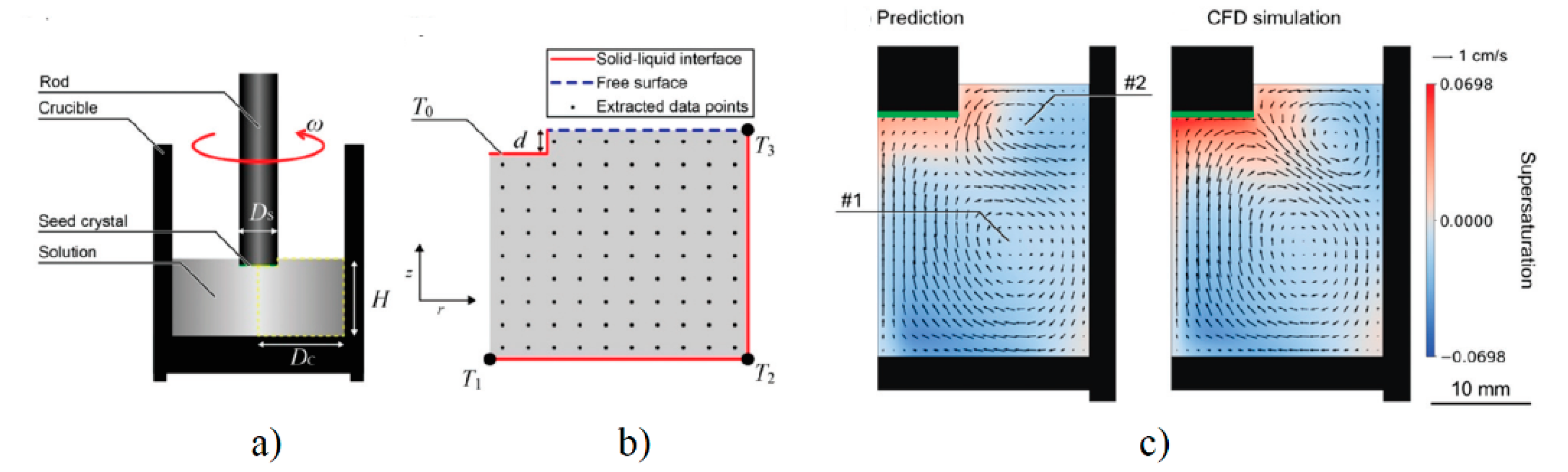
  26. Tsunooka, Y.; Kokubo, N.; Hatasa, G.; Harada, S.; Tagawa, M.; Ujihara, T. High-speed prediction of computational fluid dynamics simulation in crystal growth. CrystEngComm 2018, 20, 6546–6550. [Google Scholar] [CrossRef] [Green Version]
  27. Tang, Q.W.; Zhang, J.; Lui, D. Diameter Model Identification of CZ Silicon Single Crystal Growth Process. In Proceedings of the International Symposium on Industrial Electronics (IEEE) 2018 Chinese Automation Congress (CAC), Xi’an, China, 30 November–2 December 2018; pp. 2069–2073. [Google Scholar] [CrossRef]
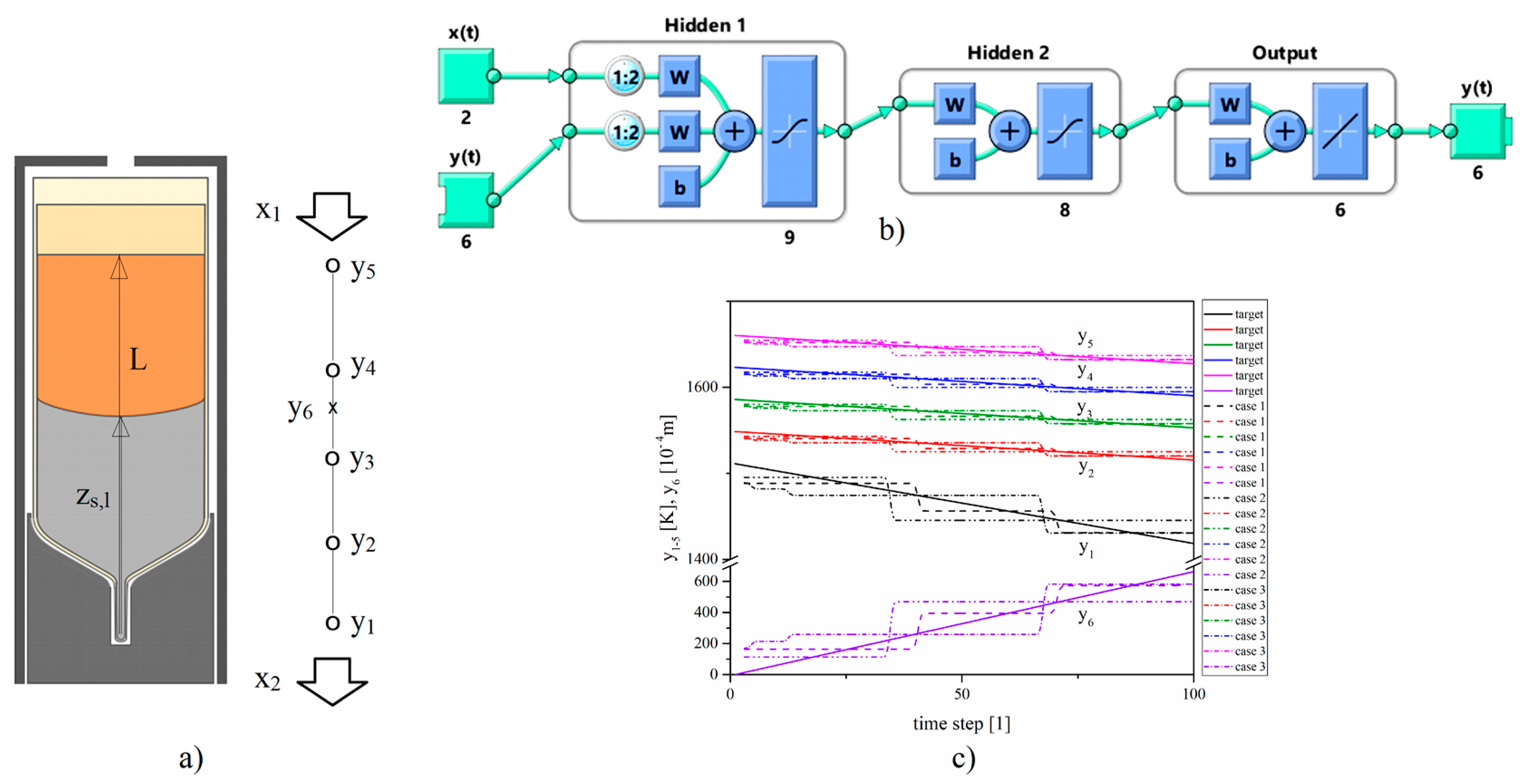
  28. Dropka, N.; Holena, M.; Ecklebe, S.; Frank-Rotsch, C.; Winkler, J. Fast forecasting of VGF crystal growth process by dynamic neural networks. J. Cryst. Growth 2019, 521, 9–14. [Google Scholar] [CrossRef]
  29. Dropka, N.; Holena, M. Optimization of magnetically driven directional solidification of silicon using artificial neural networks and Gaussian process models. J. Cryst. Growth 2017, 471, 53–61. [Google Scholar] [CrossRef]
  30. Dropka, N.; Holena, M.; Frank-Rotsch, C. TMF optimization in VGF crystal growth of GaAs by artificial neural networks and Gaussian process models. In Proceedings of the XVIII International UIE-Congress on Electrotechnologies for Material Processing, Hannover, Germany, 6–9 June 2017; pp. 203–208. [Google Scholar]
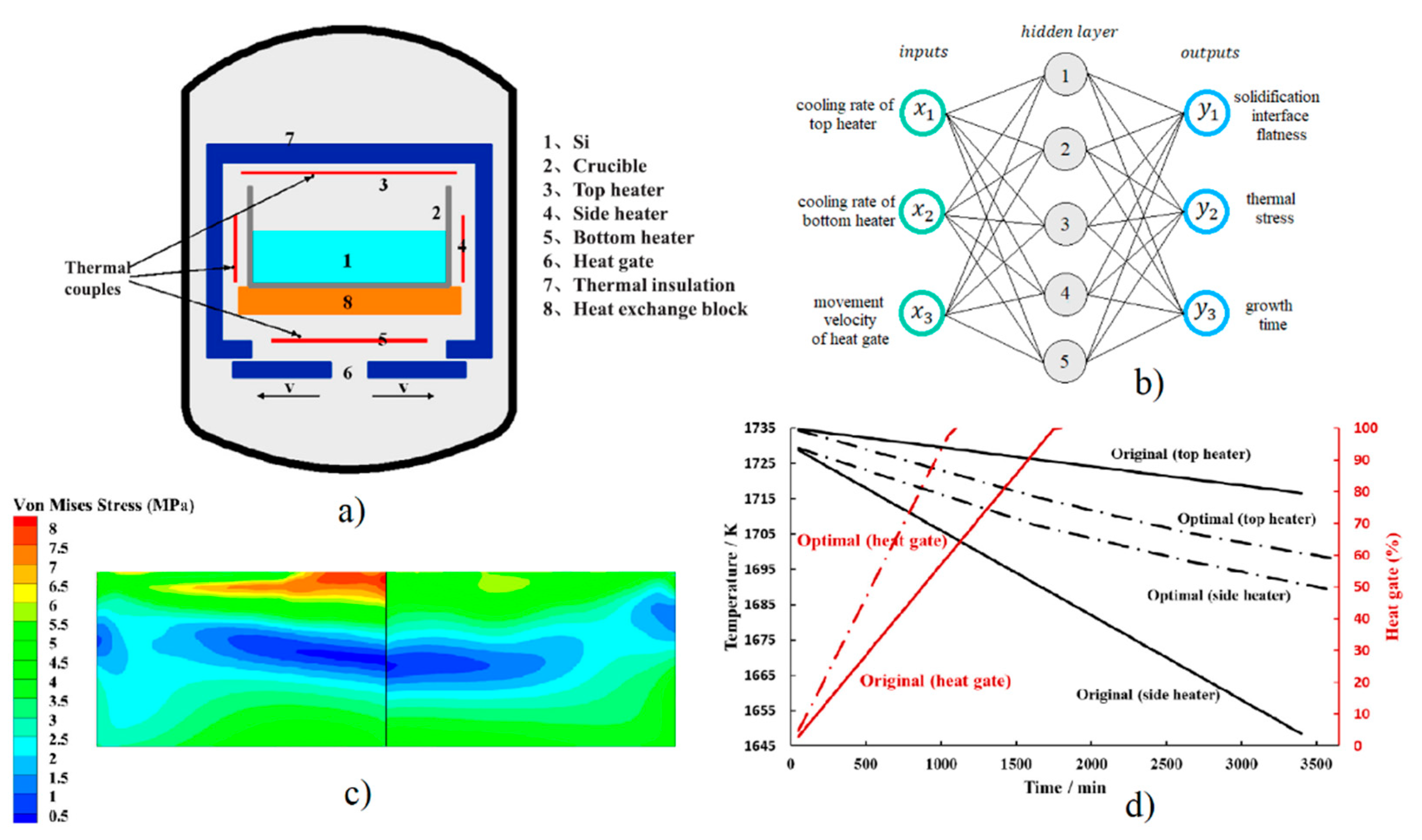
  31. Dang, Y.; Liu, L.; Li, Z. Optimization of the controlling recipe in quasi-single crystalline silicon growth using artificial neural network and genetic algorithm. J. Cryst. Growth 2019, 522, 195–203. [Google Scholar] [CrossRef]
  32. Ujihara, T.; Tsunooka, Y.; Endo, T.; Zhu, C.; Kutsukake, K.; Narumi, T.; Mitani, T.; Kato, T.; Tagawa, M.; Harada, S. Optimization of growth condition of SiC solution growth by the predication model constructed by machine learning for larger diameter. Jpn. Soc. Appl. Phys. 2019. [Google Scholar]
  33. Ujihara, T.; Tsunooka, Y.; Hatasa, G.; Kutsukake, K.; Ishiguro, A.; Murayama, K.; Narumi, T.; Harada, S.; Tagawa, M. The Prediction Model of Crystal Growth Simulation Built by Machine Learning and Its Applications. Vac. Surf. Sci. 2019, 62, 136–140. [Google Scholar] [CrossRef]
  34. Velásco-Mejía, A.; Vallejo-Becerra, V.; Chávez-Ramírez, A.; Torres-González, J.; Reyes-Vidal, Y.; Castañeda, F. Modeling and optimization of a pharmaceutical crystallization process by using neural networks and genetic algorithms. Powder Technol. 2016, 292, 122–128. [Google Scholar] [CrossRef]
  35. Paengjuntuek, W.; Thanasinthana, L.; Arpornwichanop, A. Neural network-based optimal control of a batch crystallizer. Neurocomputing 2012, 83, 158–164. [Google Scholar] [CrossRef]
  36. Samanta, G. Application of machine learning to a MOCVD process. In Proceedings of the Program and Abstracts Ebook of ICCGE-19/OMVPE-19/AACG Conference, Keystone, CO, USA, 28 July–9 August 2019; pp. 203–208. [Google Scholar]
  37. Boucetta, A.; Kutsukake, K.; Kojima, T.; Kudo, H.; Matsumoto, T.; Usami, N. Application of artificial neural network to optimize sensor positions for accurate monitoring: An example with thermocouples in a crystal growth furnace. Appl. Phys. Express 2019, 12, 125503. [Google Scholar] [CrossRef]
  38. Daikoku, H.; Kado, M.; Seki, A.; Sato, K.; Bessho, T.; Kusunoki, K.; Kaidou, H.; Kishida, Y.; Moriguchi, K.; Kamei, K. Solution growth on concave surface of 4H-SiC crystal. Cryst. Growth Des. 2016, 1256–1260. [Google Scholar] [CrossRef]
  39. Kingma, D.P.; Ba, J. Adam: A method for stochastic optimization. In Proceedings of the International Conference on Learning Representations ICLR, San Diego, CA, USA, 7–9 May 2015; pp. 1–15. [Google Scholar]
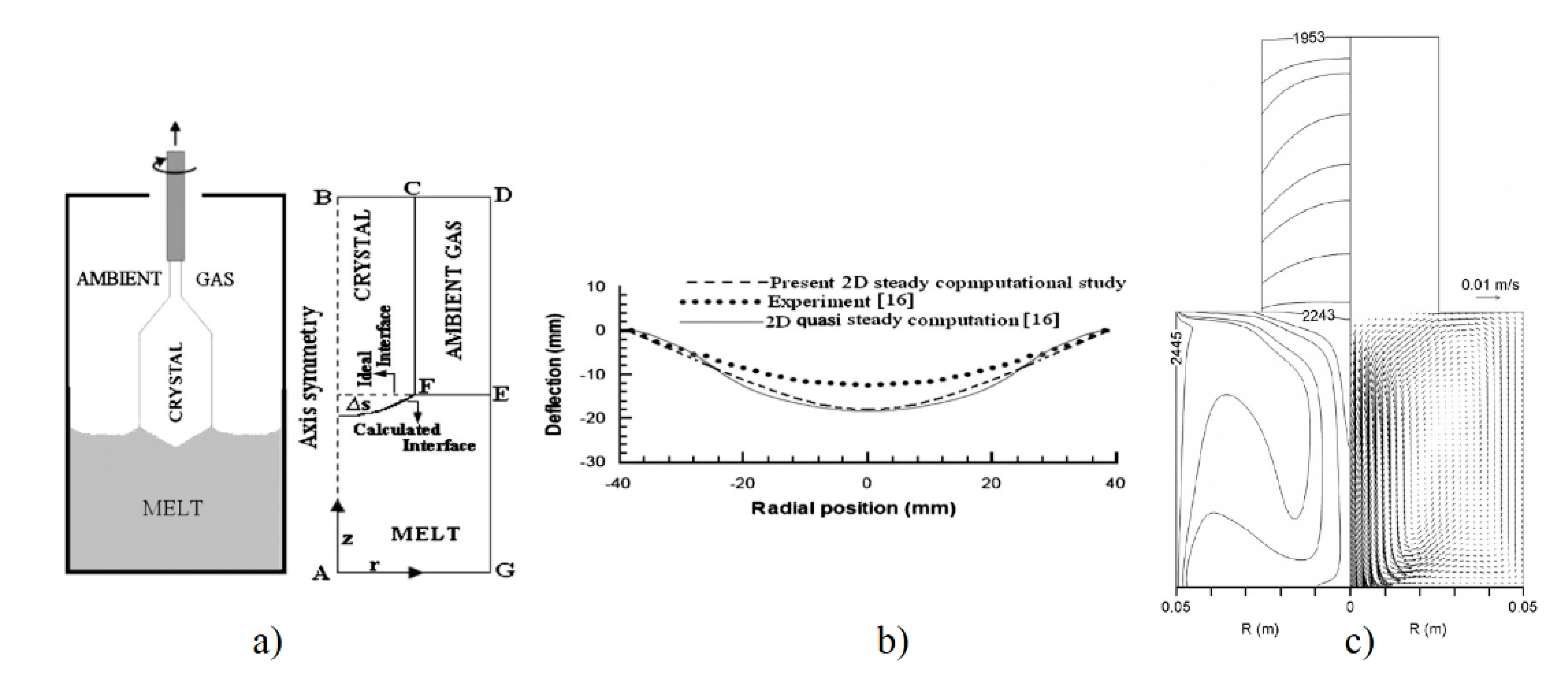
  40. Yakovlev, E.V.; Kalaev, V.V.; Bystrova, E.N.; Smirnova, O.V.; Makarov, Y.N.; Frank-Rotsch, C.; Neubert, M.; Rudolph, P. Modeling analysis of liquid encapsulated Czochralski growth of GaAs and InP crystals. Cryst. Res. Technol. 2003, 38, 506–514. [Google Scholar] [CrossRef]
  41. Duraisamy, K.; Iaccarino, G.; Xiao, H. Turbulence Modeling in the Age of Data. Annu. Rev. Fluid Mech. 2019, 51, 357–377. [Google Scholar] [CrossRef] [Green Version]
  42. Isayev, O.; Oses, C.; Toher, C.; Gossett, E.; Curtalolo, S.; Tropsha, A. Universal fragment descriptors for predicting properties of inorganic crystals. Nat. Commun. 2017, 8, 15679. [Google Scholar] [CrossRef]
  43. Xie, T.; Grossman, J.C. Crystal Graph Convolutional Neural Networks for an Accurate and Interpretable Prediction of Material Properties. Phys. Rev. Lett. 2018, 120, 145301. [Google Scholar] [CrossRef] [Green Version]
  44. Carrete, J.; Li, W.; Mingo, N.; Wang, S.; Curtalolo, S. Finding Unprecedentedly Low-Thermal-Conductivity Half-Heusler Semiconductors via High-Throughput Materials Modeling. Phys. Rev. X 2014, 4, 011019. [Google Scholar] [CrossRef] [Green Version]
  45. Seko, A.; Maekawa, T.; Tsuda, K.; Tanaka, I. Machine learning with systematic density-functional theory calculations: Application to melting temperatures of single- and binary-component solids. Phys. Rev. B 2014, 89, 054303. [Google Scholar] [CrossRef] [Green Version]
  46. Gaultois, M.W.; Oliynyk, A.O.; Mar, A.; Sparks, T.D.; Mulholland, G.; Meredig, B. Perspective: Web-based machine learning models for real-time screening of thermoelectric materials properties. APL Mater. 2016, 4, 53213. [Google Scholar] [CrossRef] [Green Version]
  47. Ziatdinov, M.; Dyck, O.; Maksov, A.; Li, X.; Sang, X.; Xiao, K.; Unocic, R.R.; Vasudevan, R.; Jesse, S.; Kalinin, S.V. Deep Learning of Atomically Resolved STEM Images: Chemical Identification and Tracking Local Transformations. ACS Nano 2017, 11, 12742–12752. [Google Scholar] [CrossRef] [PubMed] [Green Version]
  48. Guven, G.; Oktay, A.B. Nanoparticle detection from TEM images with deep learning. In Proceedings of the 26th Signal Processing and Communications Applications Conference (SIU), Izmir, Turkey, 2–5 May 2018; pp. 1–4. [Google Scholar]
  49. Gal, Y.; Islam, R.; Ghahramani, Z. Deep Bayesian Active Learning with Image Data. arXiv. 2017. Available online: https://arxiv.org/abs/1703.02910 (accessed on 25 July 2020).
  50. Huang, S.-J.; Zhao, J.-W.; Liu, Z.-Y. Cost-Effective Training of Deep CNNs with Active Model Adaptation. In Proceedings of the 24th ACM SIGKDD International Conference on Knowledge Discovery & Data Mining, London, UK, 19–23 August 2018; pp. 1580–1588. [Google Scholar] [CrossRef] [Green Version]
  51. Kandemir, M. Variational closed-Form deep neural net inference. Pattern Recognit. Lett. 2018, 112, 145–151. [Google Scholar] [CrossRef]
  52. Zheng, J.; Yang, W.; Li, X. Training data reduction in ddeep neural networks with partial mutual information based feature selection and correlation matching based active learning. In Proceedings of the 2017 IEEE International Conference on Acoustics, Speech and Signal Processing (ICASSP), New Orleans, LA, USA, 5 March 2017; pp. 2362–2366. [Google Scholar] [CrossRef]
  53. Sutskever, I.; Vinyals, O.; Le, Q.V. Sequence to sequence learning with neural networks. NIPS 2014, 3104–3112. [Google Scholar]
Figure 1. Architecture of various types of neural networks. Reprinted from [10] with permission from F.Van Veen & S. Leijnen.
Crystals 10 00663 g001
Figure 2. Example of a feed-forward ANN: (a) neuron, (b) architecture.
Crystals 10 00663 g002
Figure 3. Example of a recurrent NARX ANN architecture with 1 hidden layer, m neurons and n time delays.
Crystals 10 00663 g003
Figure 4. Example of CNN for material property prediction. Reprinted from [17] with permission from MDPI.
Crystals 10 00663 g004
Figure 5. Search process for the optimum when ANN and GA are coupled.
Crystals 10 00663 g005
Figure 6. Example of Gaussian process in one dimension. Reprinted from [22] with permission from The American Chemical Society.
Crystals 10 00663 g006
Figure 7. High-speed prediction of CFD simulations of supersaturation and velocity fields in top seeded SiC solution growth (TSSG) using feed forward ANN with 4 hidden layers: (a) Configuration of TSSG process, (b) computational domain in SiC for CFD, (c) Supersaturation and velocity distribution predicted by ANN (left) and by CFD (right). Reprinted from [26] with permission from the Royal Society of Chemistry.
Crystals 10 00663 g007
Figure 8. Optimization of the process parameters affecting the shape and position of crystal–melt interface in Cz-YAG crystal growth using feed-forward ANN/GA approach: (a) configuration and computational domain, (b) comparison of literature experimental and CFD predictions of interface deflection for InP with CFD predictions of interface deflection for YAG, (c) optimized temperature and velocity field. Reprinted from [18] with permission from Elsevier.
Crystals 10 00663 g008
Figure 9. Optimization of magnetic parameters in magnetically driven DS-Si using feed-forward ANN/GP: (a) CFD and magnetic simulation results for generation of database, (b) ANN architecture, (c) probability distribution of fulfilling the condition |Δ| < 0.1 mm as a function of Travelling magnetic field’s (TMF) magnetic parameters. Reprinted from [29] with permission from Elsevier.
Crystals 10 00663 g009
Figure 10. Optimization of controlling recipe in quasi-mono Si growth using feed-forward ANN coupled with GA: (a) Configuration of a G6-size industrial seeded directional solidification (DS) furnace, (b) ANN architecture, (c) thermal stress field in the grown crystals between the original controlling recipe (left) and the optimal recipe (right), (d) original and the optimal growth recipe. Reprinted from [31] with permission from Elsevier.
Crystals 10 00663 g010
Figure 11. Fast forecasting of dynamic growth recipe in VGF-GaAs growth using NARX-ANN: (a) Configuration of the computational domain, (b) NARX architecture with 2 hidden layers and 2 time delays, (c) predicted temperatures and interface position in monitoring points by an ANN. Reprinted from [28] with permission from Elsevier.
Crystals 10 00663 g011

