Properties of Fourier Syntheses and New Syntheses

Abstract

In this study, the properties of observed, difference, and hybrid syntheses (hybrid indicates a combination of observed and difference syntheses) are investigated from two points of view. The first has a statistical nature and aims to estimate the amplitudes of peaks corresponding to the model atoms, belonging or not belonging to the target structure; the amplitudes of peaks related to the target atoms, missed or shared with the model; and finally, the quality of the background. The latter point deals with the practical features of Fourier syntheses, the special role of weighted syntheses, and their usefulness in practical applications. It is shown how the properties of the various syntheses may vary according to the available structural model and, in particular, how weighted hybrid syntheses may act like an observed and difference or a full hybrid synthesis. The theoretical results obtained in this paper suggest new Fourier syntheses using novel Fourier coefficients: their main features are first discussed from a mathematical point of view. Extended experimental applications show that they meet the basic mission of the Fourier syntheses, enhancing peaks corresponding to the missed target atoms, depleting peaks corresponding to the model atoms not belonging to the target, and significantly reducing the background. A comparison with the results obtained via the most popular modern Fourier syntheses is made, suggesting a role for the new syntheses in modern procedures for phase extension and refinement. The most promising new Fourier synthesis has been implemented in the current version of SIR2014.

1. Introduction

Since 1929, when Bragg demonstrated the usefulness of Fourier syntheses for the solution of a diopside crystal structure [1], their calculation has become a central step in phasing and/or phase refinement procedures. Fourier syntheses lose their role when the structure is solved by cryo-electron microscopy, but they are still central when experimental diffraction data are collected, for example, in the case of X-ray free electron laser or synchrotron data, when more traditional and more popular ab initio, molecular replacement, and anomalous dispersion techniques are used. Many types of Fourier syntheses may be used, according to the specific purpose of the calculations: their variety (up to the 1970′s) may be observed in the textbook by Ramachandran and Srinivasan [2], which is entirely dedicated to the subject. We anticipate the meaning of the symbols more frequently used in this paper. According to Equation (1):

$$F={\sum }_{j=1}^N{f}_{j}exp\left(2\pi ih{r}_j\right)=\left|F\right|exp\left(i\phi \right)$$

(1)

F is the structure factor of the target structure; its modulus corresponds to the observed structure factor. N is the number of atoms in the unit cell of the target structure, and $f_j$, j = 1, …., N represent the corresponding atomic scattering (thermal parameters included). Furthermore (Equation (2)),

$$F_p={\sum }_{j=1}^p{f}_{j}exp\left(2\pi ih{r}_{pj}\right)=\left|F_p\right|exp\left(i{\phi }_p\right)$$

(2)

is the structure factor of the model structure, where $r_{pj}=r_j+\Delta r_j$. $\Delta r_j$ is the misfit between the jth atomic positions in the target and the model structures, and p is the number of atoms in the corresponding unit cell. In this paper $F_p$ is the structure factor available by the application of molecular replacement methods, or by subsequent phase refinement.

Today, only a few types of syntheses survive in modern crystallographic programs.

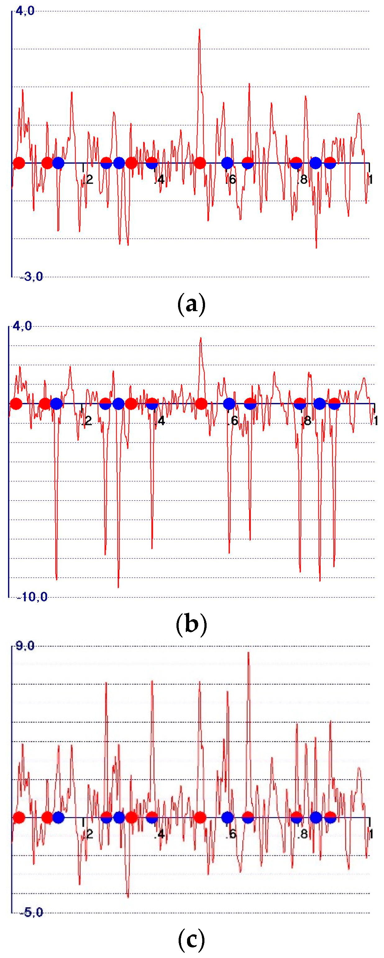
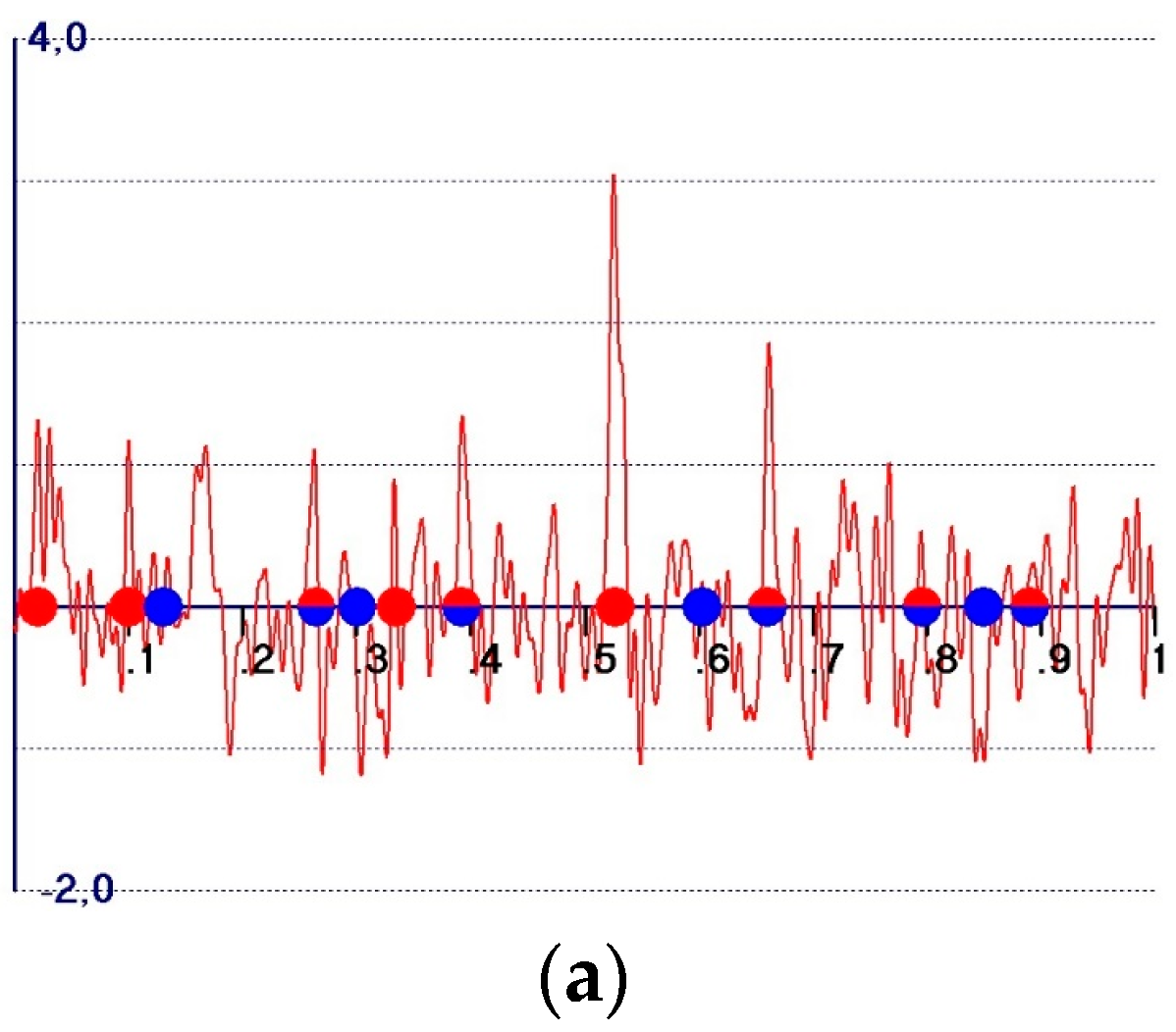
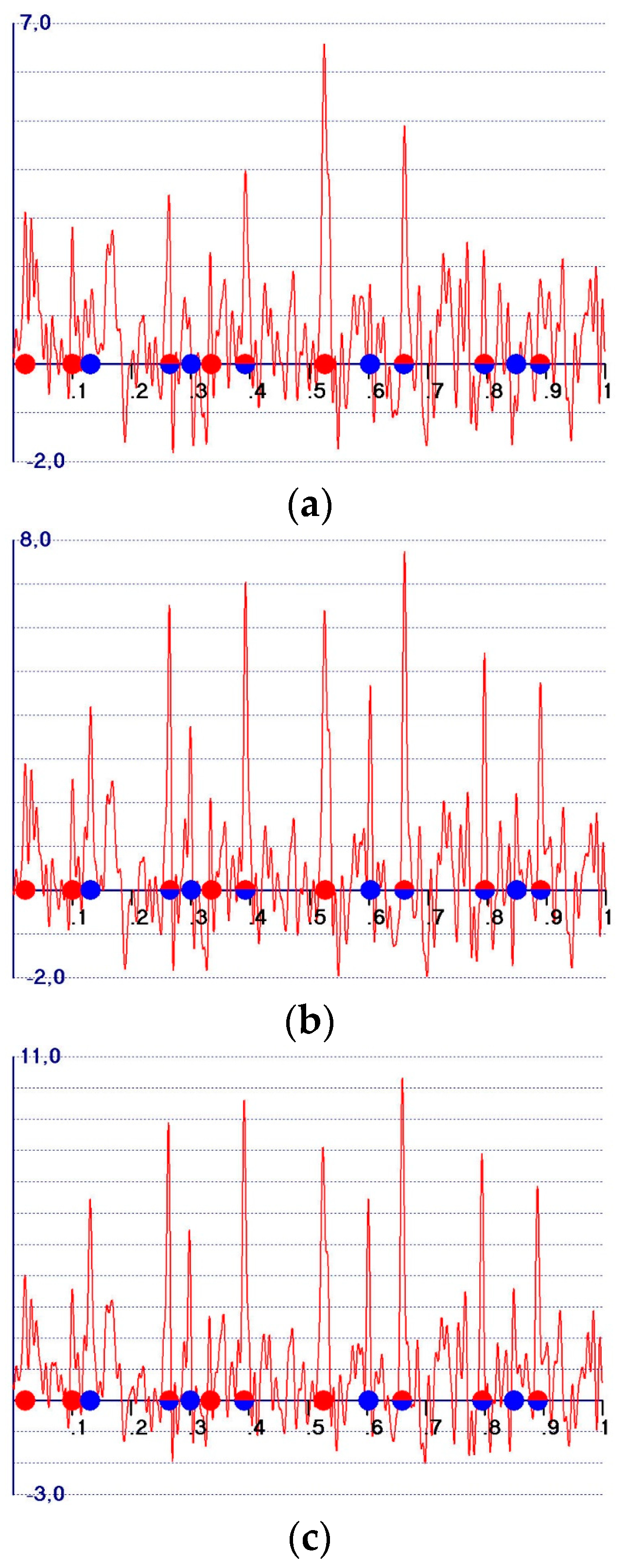
(a)

The so-called observed Fourier syntheses (Formula (3))

$$\left|F\right|exp\left(i{\phi }_p\right)$$

(3)

as the Fourier coefficient. They soon became obsolete, and were replaced by the observed weighted syntheses [3,4,5,6,7,8,9,10,11] with (Formula (4)):

$$m\left|F\right|exp\left(i{\phi }_p\right)$$

(4)

as Fourier coefficients, where m reflects the probability that the model phase is close to the target phase. m is usually estimated according to Sim [12] or Srinivasan [13]. They play a central role in any modern edm procedure.

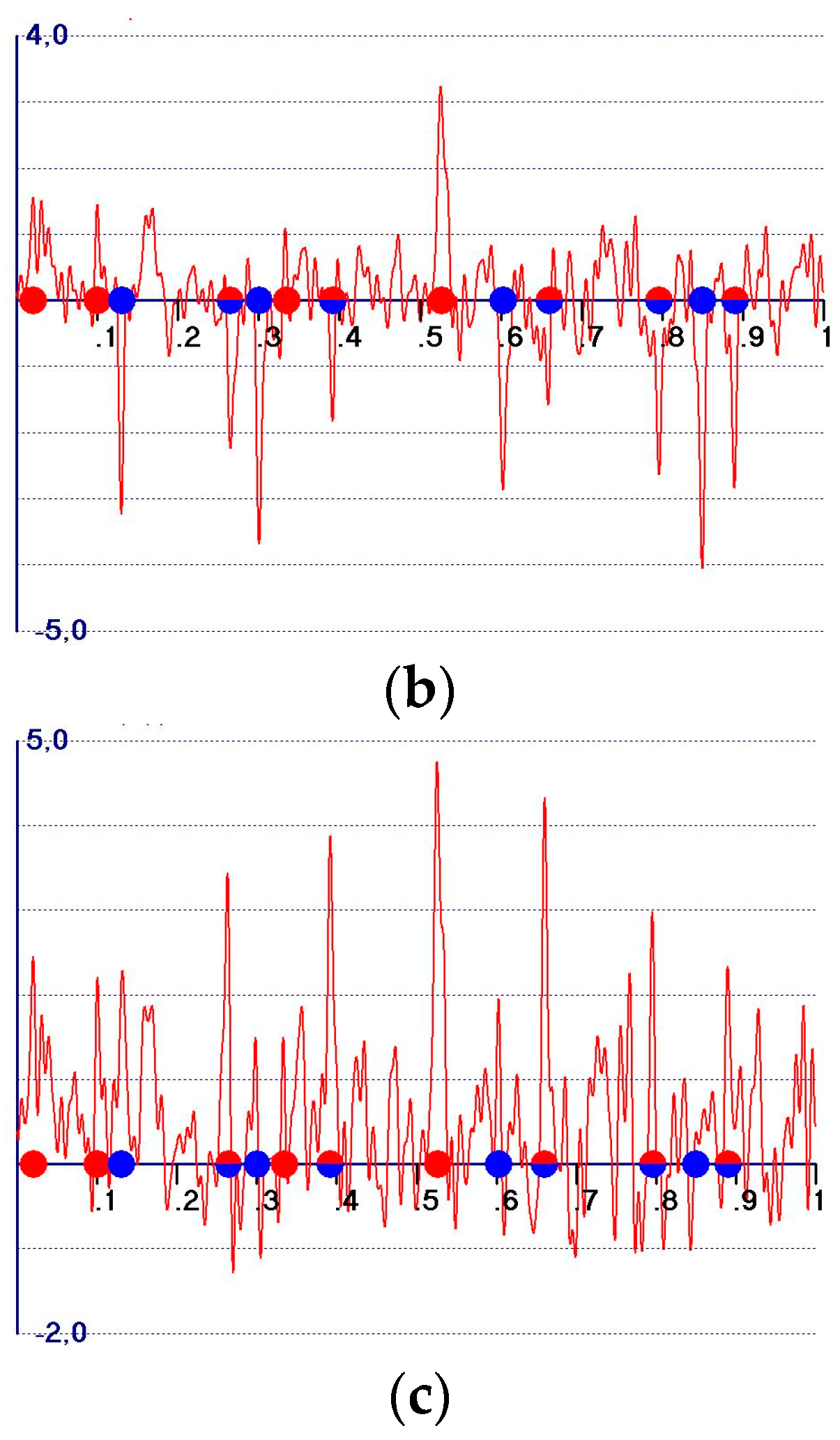
(b)

The difference electron density (Formula (5)), using

$$\left(\left|F\right|-\left|F_p\right|\right)exp\left(i{\phi }_p\right)$$

(5)

as Fourier coefficients. Its properties were extensively studied by [14,15,16]. Caliandro et al. [17,18,19] suggested an iterative refinement procedure involving both difference and observed Fourier syntheses, generalizing current edm procedures.

(c)

Main [20] proposed (Formula (6))

$$\left(m\left|F\right|-\left|F_p\right|\right)exp\left(i{\phi }_p\right)$$

(6)

as the coefficient of difference synthesis. A more recent probabilistic approach [21] generalized Main’s formula for the case in which the target and model have different scattering powers, and used it in the so-called VLD (Vive la Difference) phasing procedure [22,23,24].

(d)

Read [25], on the basis of maximum likelihood considerations, suggested, for difference Fourier synthesis, the coefficient (Formula (7))

$$\left(m\left|F\right|-D\left|F_p\right|\right)exp\left(i{\phi }_p\right)$$

(7)

(e)

More recently, the difference Fourier synthesis proposed by Burla et al. [26] used (Formula (8))

$${\left[{\left|F\right|}^2+{\left|F_p\right|}^2-2m\left|F\right|\left|F_p\right|\right]}^{1/2}$$

(8)

as the Fourier coefficient amplitude (it is the expected amplitude of the difference ${\left|F-F_p\right|}^2$), and the phase ${\phi }_p$ if $\left|F\right|>\left(2-\sqrt{m}\left|F_p\right|\right)$, or ${\phi }_p+\pi$ if $\left|F\right|<\left(2-\sqrt{m}\left|F_p\right|\right)$.

The difference syntheses mentioned above belong to the family of hybrid syntheses, which combine observed and difference syntheses through suitable integral coefficients (e.g., $\left(2\left|F\right|-\left|F_p\right|\right)exp\left(i{\phi }_p\right)$ or $\left(\left|F\right|-2\left|F_p\right|\right)exp\left(i{\phi }_p\right)$ may be used as Fourier coefficients). We will show that the observed synthesis is in itself a combination of other syntheses.

The greater effectiveness of the phasing procedures is obtained by weighted hybrid syntheses (see the next sections). Today, the general properties of the weighted and unweighted Fourier syntheses are substantially known. However, a mathematical treatment able to estimate the expected amplitudes of the peaks related to the target atoms and/or the model atoms and the quality of the background is still not available. One of the latest contributions on the matter is that of Vijayan [27], who, using the theory of Ramachandran and Srinivasan [2], estimated that the peak amplitude in the point $r_{pj}$ of a difference electron density map is proportional to $f_j\left[\left({\mathsf{\Sigma }}_N/2{\mathsf{\Sigma }}_p\right)-1\right]$. However, the estimate is very rough because it does not involve the quality of the model structure and therefore the average phase error.

The mathematical approach described in this paper is able to provide the properties of each Fourier synthesis as an explicit function of the atomic misfit between the model and the target positions, of the average phase error, of the prior knowledge of the atomic scattering factors, and of the data resolution. Such an approach will clarify the predictive power of each synthesis, in particular, the capacity for predicting the positions of the target missing atoms and the positions of the wrongly located model atoms. That is the first purpose of this paper. The second aim is to verify if, in addition to the most popular syntheses used today, new ones can be found with good and/or unexpected properties, e.g., if some of them can help in the difficult transition from an imperfect model to the target structure. For this purpose, the new Fourier syntheses proposed in this paper have been implemented in the current version of SIR2014 and applied to practical cases (experimental data resolution in the range of 1.57–2.95 Å).

2. The Observed Fourier Synthesis

It is normal to write the structure factor of a given target structure as (Equation (9))

$$F_h={{\displaystyle \sum }}_{j=1}^N{f}_{j}exp\left(2\pi ih{r}_j\right)=\left|F_h\right|exp\left(i{\phi }_h\right)$$

(9)

where the vector $r_j$ defines the target atomic positions and $f_j$ represents the corresponding atomic scattering factors calculated for the given reflection h. It is also normal to represent the target electron density by (Equation (10))

$$\rho \left(r\right)=\frac{1}{V}{{\displaystyle \sum }}_h{F}_{h}exp\left(-2\pi ihr\right)$$

(10)

where $\left|F_h\right|$ is the observed structure factor amplitude.

Introducing Equation (9) into Equation (10) allows one to study the behavior of the electron density versus the atomic positions (Equation (11)):

$$\rho \left(r\right)=\frac{1}{V}{{\displaystyle \sum }}_h{{\displaystyle \sum }}_{j=1}^N{f}_{j}exp\left[2\pi ih\left(r_j-r\right)\right]=\frac{2}{V}{{\displaystyle \sum }}_h{{\displaystyle \sum }}_{j=1}^N{f}_j\cos \left[2\pi h\left(r_j-r\right)\right]$$

(11)

For Equation (11), as well as for all of the related following expressions, it is implicitly assumed that, when the cosine function is used, the summation over h excludes Friedel opposite reflections.

When r coincides with one of the atomic positional vectors, e.g., when $r=r_j$ (Equation (12)), we have

$$\rho \left(r_j\right)=\frac{2}{V}{{\displaystyle \sum }}_h{f}_j+\frac{2}{V}{{\displaystyle \sum }}_h{{\displaystyle \sum }}_{k\ne j=1}^N{f}_k\cos \left[2\pi h\left(r_k-r_j\right)\right]$$

(12)

Since the contribution of the second term on the right hand side of Equation (12) is statistically negligible when h uniformly varies over all of the measured reflections (this hypothesis will always be valid in this paper), it may be stated as presented in Equation (13):

$$\rho \left(r\right)=\frac{2}{V}{{\displaystyle \sum }}_h{f}_j\left(h\right)$$

(13)

For $r\ne r_j$, no remarkable background is present outside of the target atom positions: the electron density vanishes everywhere except for the resolution ripples close to the $r_j$. This does not occur if Equation (11) involves a summation on a subset of the experimental indices: for example, in the case of pseudo-translational symmetry with pseudo-translation vector $u=a/3$, if there are two heavy atoms in positions $r$ and $r+a/3$, a non-vanishing electron density at $r+2a/3$ may be found if only reflections with h = 3n are used in Equation (11). In this study, we will always assume that the h reflections are uniformly distributed in the reciprocal space.

Let us now consider an imperfect model structure, whose atomic positions are defined by the $r_{pj}=r_j+\mathsf{\Delta }{r}_j$ vectors. Then, the value of the calculated (from the model) electron density in a general point r (Equation (14)) will be

$${\rho }_p\left(r\right)=\frac{2}{V}{{\displaystyle \sum }}_h{{\displaystyle \sum }}_{j=1}^p{f}_j\cos \left[2\pi h\left(r_{pj}-r\right)\right]$$

(14)

The ${\rho }_p\left(r\right)$ maxima will vanish in all points of the unit cell, except at the model atomic positions: at $r_{pj}$, the density amplitude will be (Equation (15)):

$${\rho }_p\left(r_{pj}\right)=\frac{2}{V}{{\displaystyle \sum }}_h{f}_j\left(h\right)$$

(15)

which is perfectly equal to Equation (13). Obviously, this model density also does not show any remarkable background except for the resolution ripples surrounding the model atoms.

Quite often, when a molecular model is not available and only a model electron density is attainable, it is difficult to evaluate how many atoms are included in the current model. It is then frequently assumed that N~p: this is the approximation we will adopt.

In this paper, we will make use of figures showing a one-dimensional simple target and model densities for various Fourier syntheses. The figures cannot accurately represent the large variety of three-dimensional syntheses which may be found in practical cases, but they are a useful didactical tool for checking and describing the main properties of the syntheses. In particular, we will use two pairs of one-dimensional target-model structures consisting of nine atoms each. In the first case, five atoms of the model overlap with the target atoms, and in the second case, only three model atoms overlap with the target atoms.

Figure 1a shows the calculated electron densities for the first pair of target-model structures. The red lines correspond to the target density and the red circles denote the target atomic positions. In the same figure, the blue lines correspond to the model density and the blue circles denote the model atomic positions. Five atomic positions of the model structure perfectly overlapping with five target atoms are marked by red-blue circles (this notation will be maintained for all of the figures). The peak intensities agree with Equations (13) and (15).

Let us now consider again the case of an imperfect model: we want to calculate the so-called observed Fourier synthesis, as is usually done when the model is under refinement (Equation (16)). In this case,

$${\rho }_o\left(r\right)=\frac{1}{V}{{\displaystyle \sum }}_h\left|F_h\right|exp\left(i{\phi }_{ph}\right)exp\left(-2\pi ihr\right)$$

(16)

In Equation (16), the best approximation of the target phase (say ${\phi }_{ph}$) is combined with the experimental estimate of the target structure factor. What do crystallographers want from this synthesis? Let us distinguish four types of peaks:

T.no.M peaks, corresponding to the target atomic positions and not included in the set the model atoms;

M.no.T peaks, corresponding to the model atomic positions which are not part of the target structure;

T&M peaks, corresponding to the model and the target atomic positions;

No.T.no.M false peaks, without any correspondence with the model and the target atoms.

A good observed density is expected to emphasize the amplitudes of the T.no.M and T&M peaks, deplete the amplitudes of the M.no.T, and make the intensity of the No.T no.M peaks negligible.

Let us see if these expectations may be satisfied by our mathematical approach. If we assume ${\phi }_{ph}={\phi }_h+\mathsf{\Delta }{\phi }_h$, Equation (16) may be rewritten as Equation (17):

$$\begin{array}{c}{\rho }_o\left(r\right)=\frac{1}{V}{{\displaystyle \sum }}_h{{\displaystyle \sum }}_{j=1}^N{f}_{j}exp\left(2\pi ih{r}_j\right)exp\left(i{\phi }_h+i\mathsf{\Delta }{\phi }_h\right)exp\left(-2\pi ihr\right)\\ =\frac{1}{V}{{\displaystyle \sum }}_h\left\{exp\left(i\mathsf{\Delta }{\phi }_h\right){{\displaystyle \sum }}_{j=1}^N{f}_{j}exp\left[2\pi ih\left(r_j-r\right)\right]\right\}\end{array}$$

(17)

If we multiply the two exponentials and return to the cosine formulation (the sum over h now refers to reflections not Friedel related), we obtain Equation (18):

$${\rho }_o\left(r\right)=\frac{2}{V}{{\displaystyle \sum }}_h\left\{{{\displaystyle \sum }}_{j=1}^N{f}_j\cos \left[\mathsf{\Delta }{\phi }_h+2\pi h\left(r_j-r\right)\right]\right\}$$

(18)

Equation (18) provides us with the observed electron density in any general point of the unit cell and in a form which depends on the phase errors. Let us now calculate the observed electron density at the target and model atomic positions $r_j$ and $r_{pj}$, respectively (Equations (19) and (20)):

$${\rho }_o\left(r_j\right)=\frac{2}{V}{{\displaystyle \sum }}_h{f}_j\cos \left(\mathsf{\Delta }{\phi }_h\right)+\frac{2}{V}{{\displaystyle \sum }}_h\left\{{{\displaystyle \sum }}_{k\ne j=1}^N{f}_k\cos \left[\mathsf{\Delta }{\phi }_h+2\pi h\left(r_j-r_k\right)\right]\right\}$$

(19)

and

$${\rho }_o\left(r_{pj}\right)=\frac{2}{V}{{\displaystyle \sum }}_h{f}_j\cos \left(\mathsf{\Delta }{\phi }_h-2\pi h\mathsf{\Delta }{r}_j\right)+\frac{2}{V}{{\displaystyle \sum }}_h\left\{{{\displaystyle \sum }}_{k\ne j=1}^N{f}_k\cos \left[\mathsf{\Delta }{\phi }_h+2\pi h\left(r_j-r_{pk}\right)\right]\right\}$$

(20)

Equations (19) and (20) describe the main expected features of the observed Fourier synthesis and provide the key for the success and the limits of the observed electron density in crystallographic applications.

The presence of the $\mathsf{\Delta }{\phi }_h$ shift angle in Equations (19) and (20) does not allow simple expressions for the expected values of the amplitudes at the target and model atomic positions (say $r_j$ and $r_{pj}$, respectively) to be directly derived. In Appendix A, we describe a statistical treatment able to evaluate the amplitudes (19) and (20). For the sake of simplicity, we will use there normalized structure factors. Since the observed synthesis features do not substantially vary if we use or do not use normalized structure factors, the generalization to structure factors of the statistical formulas derived in Appendix A is very simple. Two trivial modifications are needed: $\frac{1}{\sqrt{N}}$ (scattering factor of the normalized structure factors) is replaced by $f$, and $N_{refl}$ is substituted by a sum on the number of observed reflections. Therefore, from the previous results and the Appendix A equations, we can finally obtain the following.

-

The perfect target electron density (Equation (21)); the expected amplitude at the target atomic positions is

$$\langle \rho \left(r_j\right)\rangle =\frac{2}{V}{{\displaystyle \sum }}_h{f}_j$$

(21)

-

The model electron density (Equation (22)); the expected amplitude at the model atomic positions is

$$\langle \rho \left(r_{pj}\right)\rangle =\frac{2}{V}{{\displaystyle \sum }}_h{f}_j$$

(22)

-

The observed electron density (Equation (23)); the expected amplitude at the model atomic positions is

$$\langle {\rho }_o\left(r_{pj}\right)\rangle =\frac{2}{V}{{\displaystyle \sum }}_h\left[\frac{\pi }{4}+\left(1-\frac{\pi }{4}\right){\sigma }_A^2\right]f_j$$

(23)

-

The observed electron density (Equation (24)); the expected amplitude at the target atomic positions is

$$\langle {\rho }_o\left(r_j\right)\rangle =\frac{2}{V}{{\displaystyle \sum }}_h{f}_j\cos \left(\mathsf{\Delta }{\phi }_h\right)$$

(24)

Equations (21)–(24) suggest the following:

(1)

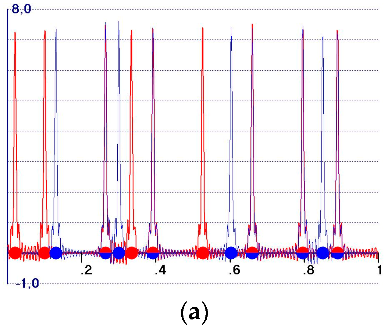
All of the peaks, Equations (23) and (24) included, are expected to be positive;

(2)

A background, practically absent in calculated electron density maps, is present. We call the background the distribution of the electron density outside the model peaks: in the background, it is normal to find peaks corresponding to the target atoms not included int the model, as well as false peaks. The source of the background is quite clear: if $\left\{\left|F\right|\right\}$ and $\left\{\phi \right\}$ are the sets of amplitudes and phases for a given crystal structure, respectively, the Fourier transform of $\left|F\right|exp\left(i\phi \right)$ will provide a vanishing electron density outside the model peaks. Any modification of the amplitudes and/or of the phases will create a background which no longer vanishes outside the model atomic peaks (examples are given in the following sections);

(3)

Target and model peaks exhibit quite different behavior, unless the peak is related to both the structures;

(4)

The expected amplitudes of the model peaks are given by Equation (23). They are always large and well-distinguishable from the background, and vary in a small range $\left[\frac{2}{V}\frac{\pi }{4}{\displaystyle \sum }_h{f}_j,\frac{2}{V}{\displaystyle \sum }_h{f}_j\right]$; the low limit is attained for a random model structure, and the high limit is obtained for a high quality model structure. The amplitude value is a smooth function of ${\sigma }_A^2$;

(5)

The expected amplitudes of the peaks corresponding to the target atoms (not part of the model) are given by Equation (24). They may vary in a large range $\left[0,\frac{2}{V}{\displaystyle \sum }_h{f}_j\right]$, according to the model quality. For bad or medium quality models, they are hardly distinguishable from the other background peaks, and only for good models are they comparable with the model amplitudes.

Figure 1b shows the observed electron density for the same one-dimensional target-model pair used in Figure 1a: the missed target atoms are in general dipped into the background because of the moderately large phase error. A real distinction between the model atoms which are not part of the target and the target atoms which are part of the model cannot be easily made at this stage as they show very similar amplitudes.

Figure 2a displays the observed density corresponding to the second one-dimensional target-model pair (only three of the nine model atoms overlap with the target atoms). As expected, a more noisy background is present, so locating the missed target atoms is more complicated than in Figure 1b.

3. The Difference Fourier Synthesis

The ideal difference synthesis should use the following Fourier coefficients (Equation (25)):

$$F_q=F-F_p=\left|F\right|exp\left(i\phi \right)-\left|F_p\right|exp\left(i{\phi }_p\right)$$

(25)

The corresponding electron density (say ${\rho }_q=\rho -{\rho }_p$) is expected to show large peaks at the positions of the target atoms which are not included in the model, to have negative peaks for the model atoms in false positions, and to vanish at the target atomic positions which are part of the model.

Since $\phi$ is unknown, it is normal to use the following substitute (Equation (26)):

$${\rho }_{1-1}\left(r\right)=\frac{1}{V}{{\displaystyle \sum }}_h\left(\left|F_h\right|-\left|F_{ph}\right|\right)exp\left(i{\phi }_{ph}\right)exp\left(-2\pi ihr\right)$$

(26)

The unusual ${\rho }_{1-1}\left(r\right)$ $\mathrm{notation}$ in Equation (26) is due to the fact that in the following sections of this paper, we will also study the so-called hybrid Fourier syntheses, in particular, the 2–1 and 1–2 syntheses, whose electron densities will be denoted by ${\rho }_{2-1}\left(r\right)$ and ${\rho }_{1-2}\left(r\right)$, respectively.

What do crystallographers want to obtain from a ${\rho }_{1-1}$ synthesis? The algebraic expression of ${\rho }_{1-1}$ suggests that for a good difference synthesis, the following should apply:

(1)

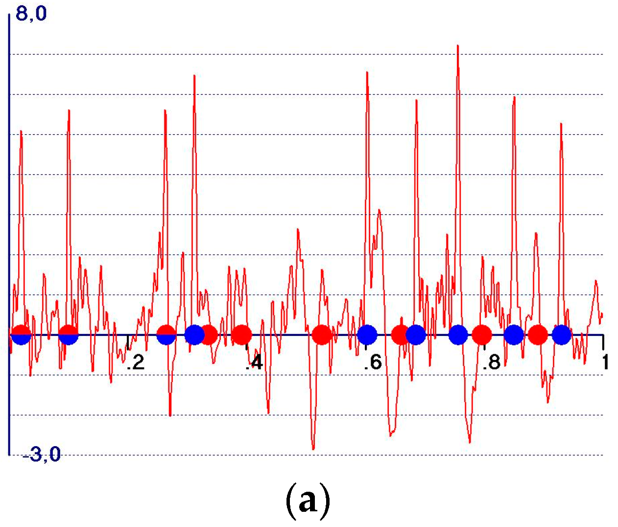
M.no.T peaks should be negative and strong;

(2)

T&M peaks should be weakly negative or, better, weakly positive;

(3)

T.no.M peaks should be positive and possibly large;

(4)

noT.no.M peaks should be vanishing.

These expectations may not always be satisfied. Indeed, in accordance with Section 2, we may rewrite Equation (26) as Equation (27):

$${\rho }_{1-1}\left(r\right)=\frac{2}{V}{{\displaystyle \sum }}_h{{\displaystyle \sum }}_{j=1}^N{f}_j\cos \left[\mathsf{\Delta }{\phi }_h+2\pi h\left(r_j-r\right)\right]-\frac{2}{V}{{\displaystyle \sum }}_h{{\displaystyle \sum }}_{j=1}^N{f}_j\cos \left[2\pi h\left(r_{pj}-r\right)\right]$$

(27)

so that (Equation (28)):

$${\rho }_{1-1}\left(r\right)={\rho }_o\left(r\right)-{\rho }_p\left(r\right)$$

(28)

Equation (27) provides the difference in electron density for any general point of the unit cell and in a form which depends on the phase errors. The use of Equation (28) allows us to describe the properties of the difference synthesis by using the results obtained for the observed and calculated syntheses:

(i)

The expected peak amplitude corresponding to a model atom is equal (subtract Equation (22) from Equation (23)) to Equation (29):

$$\langle {\rho }_{1-1}\left(r_{pj}\right)\rangle =\frac{-2}{V}{{\displaystyle \sum }}_h\left[\left(1-\frac{\pi }{4}\right)\left(1-{\sigma }_A^2\right)\right]f_j$$

(29)

Since $1-\frac{\pi }{4}\approx 0.21,$ the amplitudes at the model atomic positions are expected to be weakly negative: they asymptotically tend to vanish when the model is of a high quality (then ${\sigma }_A$ is close to 1);

(ii)

The expected peak amplitude corresponding to a target atom (which is not part of the model) coincides with the expected value of the same peak in the observed density (Equation (30)),

$$\langle {\rho }_{1-1}\left(r_j\right)\rangle =\frac{2}{V}{{\displaystyle \sum }}_h{f}_j\cos \left(\mathsf{\Delta }{\phi }_h\right)$$

(30)

because the corresponding amplitude in the calculated density is zero;

(iii)

In accordance with Section 2, the background present in the difference synthesis essentially coincides with that of the observed density. As a consequence, the missed target atoms remain hidden in the background, with weakly positive peak amplitude values. The basic advantage of the difference synthesis is that model peaks are expected to be weakly negative, so identification of the missed atoms among the positive peaks is easier.

The difference synthesis (Equation (27)) is shown in Figure 3a for the same model and target structures used in Figure 1a. The reader can easily check the agreement of the figure with the theoretical expectations (Equations (29) and (30)).

4. General Expression for Hybrid Syntheses

Traditional hybrid Fourier syntheses correspond to Fourier coefficients (Formula (31)) of the form

$$\left(\tau \left|F_o\right|-\omega \left|F_p\right|\right)exp\left(i{\phi }_p\right)$$

(31)

where $\tau$ and $\omega$ are integral numbers. Their density map exactly corresponds to Equation (32)

$${\rho }_{\tau -\omega }\left(r\right)=\tau {\rho }_o\left(r\right)-\omega {\rho }_p\left(r\right)$$

(32)

In accordance with Equation (32) it is now very easy to define the main features of these densities. Let us first consider the case $\tau <\omega$:

(i)

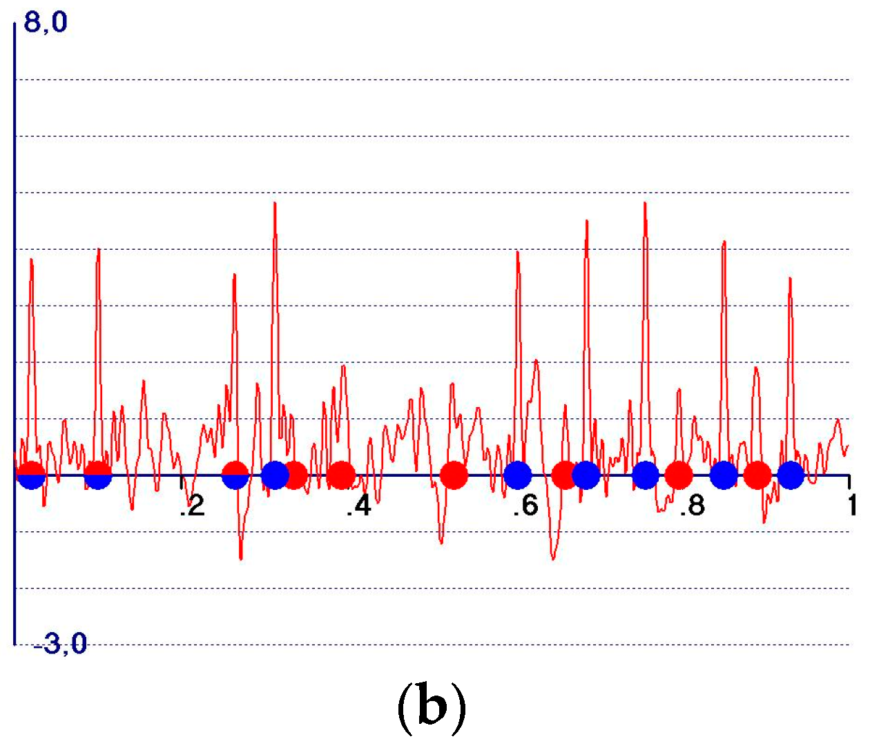
The expected peak amplitude corresponding to a model atom is equal to Equation (33)

$$\langle {\rho }_{\tau -\omega }\left(r_{pj}\right)\rangle =\frac{2}{V}{{\displaystyle \sum }}_h\left\{\tau \left[\frac{\pi }{4}+\left(1-\frac{\pi }{4}\right){\sigma }_A^2\right]-\omega \right\}{f}_j$$

(33)

Since $\frac{\pi }{4}+\left(1-\frac{\pi }{4}\right){\sigma }_A^2<1$, no matter the quality of the model, if $\tau <\omega$, then $\tau \left[\frac{\pi }{4}+\left(1-\frac{\pi }{4}\right){\sigma }_A^2\right]<\omega$, regardless of the quality of the model. The peak amplitude is therefore expected to always be negative, no matter the model quality: the greater the difference $\left|\tau -\omega \right|,$ the larger the negative amplitudes.

(ii)

The expected peak amplitude corresponding to a target atom is given by Equation (34)

$$\langle {\rho }_{\tau -\omega }\left(r_j\right)\rangle =\frac{2}{V}{{\displaystyle \sum }}_h\tau f_j\cos \left(\mathsf{\Delta }{\phi }_h\right)$$

(34)

The presence of the factor $\tau$ suggests that such amplitudes linearly increase with $\tau$, but the reader should not expect the probability of discovering target atoms not included in the model to be enhanced, because the background is enhanced by the same factor $\tau$(see Equation (33)).

The advantage of such hybrid synthesis is essentially the fact that the model peaks are eliminated from the set of positive peaks, and picking up the missed target atoms may be easier, particularly in automatic edm techniques. The only hybrid synthesis with $\tau <\omega$ which has found application in modern crystallography is 1–2 synthesis [24].

Let us now consider the case $\tau >\omega$. We can observe the following:

(i)

The expected peak amplitudes at the model atomic positions are positive for high quality models and remain negative for very low quality models. In the first case, a $\tau -\omega$ synthesis shares the features of an observed synthesis, and it is more similar to a difference synthesis in the second case;

(ii)

The expected peak amplitudes corresponding to a target atom are given by Equation (34): as for the $\tau <\omega$ case, the probability of discovering target atoms not included in the model is not enhanced;

(iii)

An interesting feature may be found. Equation (33) suggests that model peaks present in $\tau {\rho }_o\left(r\right)$ are also peaks of the $\tau {\rho }_o\left(r\right)-\omega {\rho }_p\left(r\right)$ map, but with smaller amplitudes. On the contrary, the amplitudes of target peaks of $\tau {\rho }_o\left(r\right)$ remain unvaried in $\tau {\rho }_o\left(r\right)-\omega {\rho }_p\left(r\right)$ (e.g., because ${\rho }_p\left(r\right)$ does not contribute to the target peaks), so their ratio with the amplitudes of the model peaks increases. Unfortunately, the other background peaks (e.g., those which do not correspond to the target atoms) also remain unvaried, so the difficulty in identifying missed atom peaks among the background false peaks still remains.

The most used hybrid synthesis with $\tau >\omega$ is 2–1 synthesis [28], which is, in practice, the sum of the observed ${\rho }_o$ and ${\rho }_{1-1}$ syntheses. Syntheses of type 3–1, 4–1, etc., are too similar to ${\rho }_o$ to be useful.

Figure 3b,c show 1–2 and 2–1 syntheses, respectively, for the same target and model structures used in Figure 1a. The reader can easily check the fitting of the figure with the mathematical expectations. Indeed, in Figure 3b, the strong negative peaks correspond to the model atoms (no matter if they are part or not part of the target structure), the missed atoms correspond to weak positive peaks, and the background is substantially identical to that of the observed and 1–1 difference syntheses. In Figure 3c, where 2–1 synthesis is shown, the model and missed target peaks are positive, and the background is emphasized, but has the same trend of the observed and 1–1 difference syntheses.

In accordance with the above considerations, there are currently two main limits for the hybrid syntheses. Firstly, only 1–2 and 2–1 hybrid syntheses have been used for practical applications. In this paper, we will show that other possible syntheses may be useful. Secondly, hybrid syntheses do not substantially change the background: changing $\tau$ and $\omega$ modifies the background scale, but not the relative amplitudes, of two background peaks. To overcome this drawback, many authors started studying weighted syntheses (Section 5 onwards).

5. The Weighted Observed Fourier Syntheses

The popularity of the observed electron density essentially arose from the following observation: during the phasing process, only $\left|F\right|$ observed diffraction amplitudes, $\left|F_p\right|$ model amplitudes, and corresponding phases ${\phi }_p$ are known. Therefore, the best approximation of the Fourier $\left|F\right|exp\left(i\phi \right)$ coefficient seems to be $\left|F\right|exp\left(i{\phi }_p\right)$.

It was soon realized that a better approximation could be found by using the probability that ${\phi }_p$ is equal to $\phi$. This is equivalent to using, for the calculation of the observed synthesis, the $m\left|F\right|exp\left(i{\phi }_p\right)$ Fourier coefficient rather than the $\left|F\right|exp\left(i{\phi }_p\right)$ coefficient. This change provides what is usually called weighted observed ${\rho }_{ow}\left(r\right)$ synthesis, which is the observed synthesis preferred by modern crystallographic packages.

An analysis of ${\rho }_{ow}\left(r\right)$ may be conducted by using the techniques employed for the analysis of unweighted observed synthesis. In practice, Equations (23) and (24) are replaced by Equations (35) and (36), respectively:

$$\langle {\rho }_{ow}\left(r_{pj}\right)\rangle =\frac{2}{V}{{\displaystyle \sum }}_{h}m\left[\frac{\pi }{4}+\left(1-\frac{\pi }{4}\right){\sigma }_A^2\right]f_j$$

(35)

and

$$\langle {\rho }_{ow}\left(r_j\right)\rangle =\frac{2}{V}{{\displaystyle \sum }}_{h}m{f}_j\cos \left(\mathsf{\Delta }{\phi }_h\right)$$

(36)

where m, as well as $f$, are reflection-dependent, even if this dependence, for simplifying the notation, has not been made explicit in the symbols.

The mF observed electron densities for the two model-target pairs are shown in Figure 1c and Figure 2b, respectively. A careful observation of such figures confirms the superiority of the weighted observed synthesis with respect to the unweighted one shown in Figure 1b. Accordingly, the use of the weight (with respect to the unweighted observed synthesis) leads to the following:

-

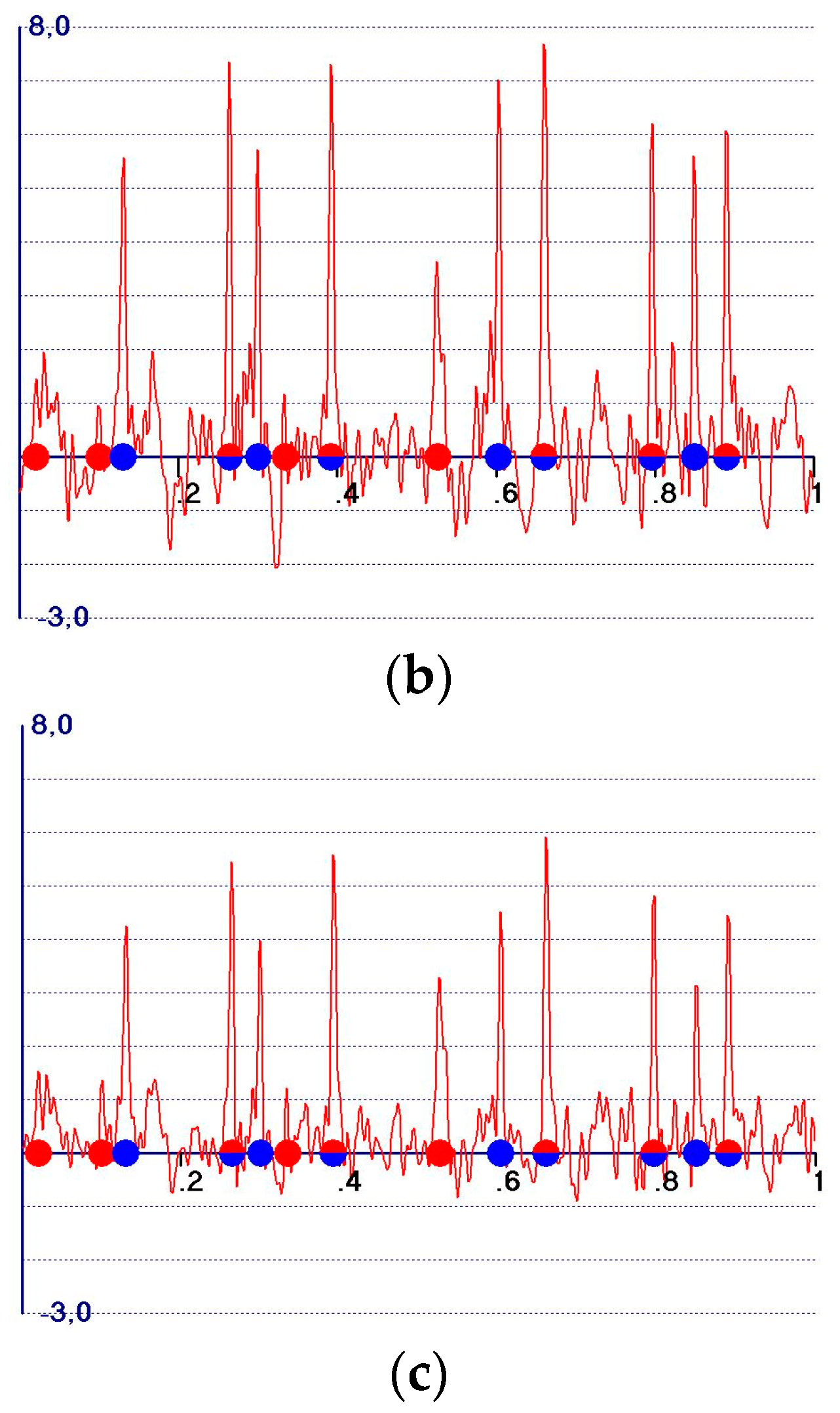
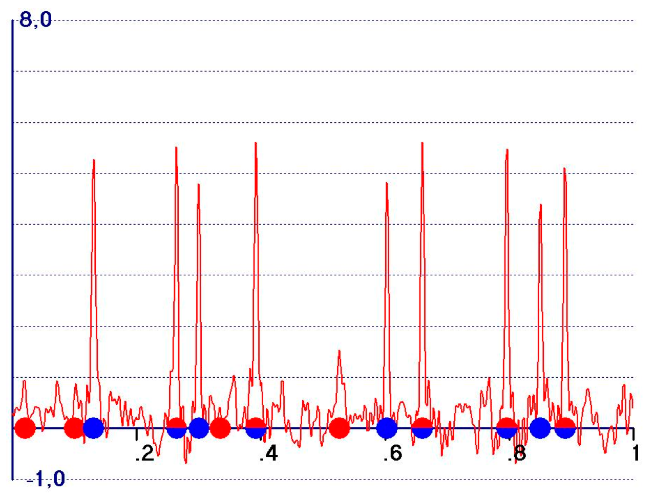
A reduction in the amplitudes of the model and target peaks, as well as the background (see Figure 1b,c). Such peaks remain positive;

-

An increase in the ratio between the amplitudes of the target and the model peaks;

-

Modification of the background of the unweighted observed synthesis and emphasis of the target peak amplitudes.

The above properties are well-known and Equations (35) and (36) finally provide numerical estimates of the peak amplitudes.

To check the properties of the weighted Fourier synthesis, the following criteria may be used:

$$CRI{T}_1={\langle I\left(j\right)\rangle }_T/{\langle I\left(j\right)\rangle }_M$$

$$CRI{T}_2={\langle I\left(j\right)\rangle }_{T.no.M}/{\langle I\left(j\right)\rangle }_{M.no.T}$$

$$CRI{T}_3={\langle I\left(j\right)\rangle }_{T.no.M}/{\langle I\left(j\right)\rangle }_{pos}$$

The letter I represents peak amplitudes, and the averages of the sets T and M are calculated for the target and model peaks, respectively. The averages of the T.no.M and M.no.T sets deal with target peaks not included in the model and model peaks which do not correspond to the target atoms, respectively. The average for the pos set is calculated for all of the pixels with a positive amplitude. The three criteria deal with the desired ability of a Fourier map to deplete the peak amplitudes of the model atoms which are not part of the target and to emphasize peak amplitudes corresponding to the missed target atoms: the higher the CRIT₁, CRIT₂, and CRIT₃ values, the greater the expected usefulness of the map. Their values, for a number of weighted and unweighted observed Fourier syntheses, are shown in

Table 1. CRIT₁, CRIT₂, and CRIT₃ are shown for various weighted and unweighted one-dimensional electron densities. Each Fourier synthesis is defined in column 1 through its Fourier coefficients (the phase component is eliminated for brevity). The values in columns 2–4 correspond to the model with five atoms perfectly overlapping with target atoms. The values in columns 5–7 correspond to the model with only three atoms overlapping with target atoms. CRIT₃ is multiplied by 100.

	Model With
	5 Overlapping Atoms			3 Overlapping Atoms
SYNTH.	CRIT1	CRIT2	CRIT3	CRIT1	CRIT2	CRIT3
F	0.71	0.29	0.18	0.45	0.21	0.19
mF	0.80	0.46	0.24	0.54	0.34	0.27
mFp	0.66	0.19	0.12	0.42	0.13	0.13
w1F	0.87	0.64	0.27	0.61	0.44	0.30
w2F	0.81	0.45	0.34	0.51	0.30	0.37
w3F	0.87	0.60	0.39	0.57	0.39	0.43
F-(1-m)Fp	0.92	0.77	0.29	0.66	0.52	0.31
F-Fp			0.43			0.40
mF-DFp			0.60			0.53
mF-Fp			0.51			0.52
<Fq>			0.49			0.41
wq<Fq>			0.48			0.41
F-mFp			0.20			0.19
mF-(1-m)Fp			0.33			0.39
m(F-Fp)			0.45			0.43
(1-m)(F-Fp)			0.35			0.28
w1|ΔF|			0.53			0.57
F-2Fp			0.46			0.44
mF-2Fp			0.50			0.54
F-2mFp			−0.03			0.01
mF-2(1-m)Fp			0.38			0.45
mF-2DFp			1.13			1.15
2F-Fp	0.92	0.76	0.28	0.65	0.53	0.28
2mF-Fp	1.69	6.65	0.39	2.31	2.48	0.46
2F-mFp	0.74	0.36	0.19	0.47	0.26	0.20
2mF-(1-m)Fp	0.95	0.84	0.29	0.71	0.58	0.34
2mF-DFp	0.98	0.95	0.35	0.61	0.45	0.36

: columns 2–4 refer to the model used in Figure 1b,c, and columns 5–7 refer to the model used in Figure 2a,b.

6. The Weighted Hybrid Fourier Syntheses

The typical coefficient of a hybrid Fourier synthesis, say $\left(\tau \left|F_o\right|-\omega \left|F_p\right|\right)exp\left(i{\phi }_p\right)$, may be weighted according to a large number of schemes: good weights are expected to improve the usefulness of the syntheses. In order to limit the possible alternatives, we will only consider Formula (37):

$$F_q=\left[\tau y_1\left(m\right)\left|F\right|-\omega y_2\left(m\right)\left|F_p\right|\right]exp\left(i{\phi }_p\right)$$

(37)

where $y_1\left(m\right)$ and $y_2\left(m\right)$ may assume various algebraic forms, limited only by the request for a reasonable simplicity and by its practical usefulness. For such synthesis, the amplitudes of the peaks corresponding to the model atoms are (Equation (38)):

$$\langle {\rho }_{\tau -\omega }\left(r_{pj}\right)\rangle =\frac{2}{V}{{\displaystyle \sum }}_h\left\{\tau y_1\left(m\right)\left[\frac{\pi }{4}+\left(1-\frac{\pi }{4}\right){\sigma }_A^2\right]-\omega y_2\left(m\right)\right\}{f}_j$$

(38)

and the amplitudes of the peaks corresponding to the target atoms are (Equation (39))

$$\langle {\rho }_{\tau -\omega }\left(r_j\right)\rangle =\frac{2}{V}{{\displaystyle \sum }}_h\tau y_1\left(m\right)f_j\cos \left(\mathsf{\Delta }{\phi }_h\right)$$

(39)

Equation (39) suggests that peaks corresponding to missed target atoms are always expected to be positive, while peak amplitudes corresponding to model atoms may be positive or negative, according to the type of synthesis (e.g., according to the $\tau$ and $\omega$ values) and the model quality. Formula (37), and consequently, Equations (38) and (39), do not imply that $\tau$ and $\omega$ are necessarily integral numbers; they may be rational numbers. In general, large values of $\omega$ increase the negativity of the model peaks and magnify the background generated by the use of the $y_2\left(m\right)$ weight (see below). Increasing $\tau$ increases the positivity of the missed target atoms and magnifies the background generated by the use of $y_1\left(m\right)$ (see below). A free use of the ratio $\omega /\tau$ may conveniently rule these effects.

Accordingly, the background of the density calculated via Formula (37) is the combination of two different backgrounds: the first is related to the background of the weighted observed synthesis and the second to the background of the weighted model synthesis. Only if the model is sufficiently good may the two background components be similar: in that case, the ${\rho }_{\tau -\omega }$ background is depleted; otherwise, it may increase at several points of the map.

In order to clarify this point, let us consider the case of the hybrid synthesis of type 1–1. While the map calculated via the $\left|F_p\right|exp\left(i{\phi }_p\right)$ coefficients has no background, the synthesis calculated via the $y_2\left(m\right)\left|F_p\right|exp\left(i{\phi }_p\right)$ coefficients should show a non-vanishing background, unless y₂(m) ≡ 1. Figure 4 shows the density calculated by using $m\left|F_p\right|exp\left(i{\phi }_p\right)$ coefficients for the same model used in Figure 1a. The background is quite visible and, in general, well-correlated, owing to the quality of the model, with the background calculated by using $m\left|F\right|exp\left(i{\phi }_p\right)$ coefficients. However, the two backgrounds may be additive in some regions and subtractive in other regions. Both the backgrounds tend to disappear for very high quality models.

One detail in Figure 4 may surprise the reader: three peaks of the background correspond to missed target atoms, in spite of the fact that structure factor amplitudes and phases of the model are used for the synthesis calculation (see also the non-negligible values of CRIT_i, for i = 1, 2, 3 in Table 1). In reality, that is not surprising: indeed, the weight m has been introduced, and this is the source of the supplementary information, because it assigns large weights to the model reflections for which ${\phi }_p\approx \phi$. Therefore, they become dominant in some way and help to reveal the position of the missed target atoms.

The use of the weight for the hybrid syntheses has a further unexpected consequence: their nature may change when the model changes. For example, $mF-F_p$ and $mF-\left(1-m\right)F_p$ syntheses simulate a $-F_p$ synthesis for quite bad models (then $m$ is very close to zero): for high quality models, $mF-F_p$ simulates a 1-1 difference synthesis and $mF-\left(1-m\right)F_p$ an observed weighted synthesis. Therefore, the usefulness of a hybrid synthesis is strictly related to the purpose of its use and the features of the model.

CRIT₃ may be used to obtain a first estimate of the usefulness of the hybrid Fourier syntheses (including the difference synthesis). Indeed, CRIT₁ and CRIT₂ criteria may be inadequate because, in hybrid syntheses, the peaks corresponding to the model atoms frequently show negative amplitudes, so the averages $\langle I{\left(j\right)\rangle }_M$ and $\langle I{\left(j\right)\rangle }_{M.no.T}$ may be close to zero or negative. However, the reader should consider all of the criteria suggested above as statistical tools more suitable for eliminating the worst syntheses than for choosing the best ones.

7. New Types of Observed Fourier Synthesis

The traditional (weighted or unweighted) observed, difference, and hybrid syntheses quoted in Section 1 cannot exhaust the list of syntheses potentially useful in modern crystallography. The research in this field ended in practice in the 90′s of the past century. The theory described so far allows us to suggest alternatives to the classical Fourier synthesis: in particular, we are interested in new forms of observed synthesis.

Reconsider the unweighted observed synthesis defined by Equation (16). It may be rewritten as Equation (40)

$$\begin{array}{c}{\rho }_o\left(r\right)=\frac{1}{V}{{\displaystyle \sum }}_h\left(\left|F_{ph}\right|+\mathsf{\Delta }{F}_h\right)exp\left(i{\phi }_{ph}-2\pi ihr\right)\\ ={\rho }_p\left(r\right)+\frac{2}{V}{{\displaystyle \sum }}_h\mathsf{\Delta }{F}_h\cos \left({\phi }_{ph}-2\pi hr\right)\end{array}$$

(40)

where $\mathsf{\Delta }{F}_h=\left|F_h|-|F_{ph}\right|$. It is easy to recognize that the observed Fourier synthesis is the sum of the model and the difference Fourier synthesis (Equation (41)):

$${\rho }_o\left(r\right)={\rho }_p\left(r\right)-{\rho }_{1-1}\left(r\right)$$

(41)

Equation (41) suggests that the superior utility of ${\rho }_o\left(r\right)$ arises from its component ${\rho }_{1-1}\left(r\right)$ (${\rho }_p\left(r\right)$ only provides information on the model), which, on the other hand, is fully responsible for the background present in ${\rho }_o\left(r\right)$. Therefore, any technique improving ${\rho }_{1-1}\left(r\right)$ may improve ${\rho }_o\left(r\right)$.

According to Equation (41), the weighted observed Fourier synthesis may be written as Equation (42)

$${\rho }_{ow}\left(r\right)=m{\rho }_o\left(r\right)=m{\rho }_p\left(r\right)+m{\rho }_{1-1}\left(r\right)$$

(42)

with Formula (43)

$$\left[m\left|F_p\right|+m\left(\left|F\right|-\left|F_p\right|\right)\right]exp\left(i{\phi }_p\right)$$

(43)

as Fourier coefficients.

Again, Formula (43) suggests that the source of the great efficiency of the observed synthesis lies in the information contained in the weighted 1-1 synthesis. We decided to increase its contribution by replacing the Formula (44)

$$m\left|F\right|=m\left|F_p\right|+m\left(\left|F\right|-\left|F_p\right|\right)$$

(44)

with Formula (45)

$$m\left|F_p\right|+m^y\left(\left|F\right|-\left|F_p\right|\right)=m^y\left|F\right|-\left(m^y-m\right)\left|F_p\right|\mathrm{with}\mathrm{y}<1$$

(45)

There are other ways in which the role of the difference synthesis may be emphasized. For example, Formula (43) may be replaced by

$$m\left|F_p\right|+ym\left(\left|F\right|-\left|F_p\right|\right)=ym\left|F\right|-\left(y-1\right)m\left|F_p\right|\mathrm{with}y>1$$

(46)

Using Formula (46) is perfectly equivalent to using Formula (47):

$$m\left|F\right|-\left(\frac{y-1}{y}\right)m\left|F_p\right|$$

(47)

The role of the difference density in the Formula (44) may also be emphasized by replacing this identity with Formula (48)

$$\left|F_p\right|+y\left(m\left|F\right|-\left|F_p\right|\right)=ym\left|F\right|-\left(y-1\right)\left|F_p\right|\mathrm{with}y>1$$

(48)

which may be rewritten as Formula (49)

$$m\left|F\right|-\left(\frac{y-1}{y}\right)\left|F_p\right|$$

(49)

Two additional syntheses deserve to be analysed. The first is a particular case of the Formula (45), occurring when $y=0$: then, the coefficient reduces to Formula (50)

$$\left|F\right|-\left(1-m\right)\left|F_p\left|\equiv m\right|F_p\right|+\left(\left|F\right|-\left|F_p\right|\right)$$

(50)

The second synthesis, formally hybrid but acting like the observed one, has Fourier coefficients (Formula (51)):

$$2m\left|F\right|-D\left|F_p\right|=m\left|F\right|+\left(m\left|F\right|-D\left|F_p\right|\right)$$

(51)

Formula (51), suggested by Read [25], is widely used in protein crystallography, and may be considered as the sum of a weighted observed synthesis and of a difference synthesis.

The syntheses with coefficients as per Formulas (45), (46), (48), (50) and (51) aim to reduce the amplitudes of the peaks corresponding to the model atoms with respect to the amplitudes of the missed target atoms. Therefore, they are expected to show similar properties, so their coefficients should be related by simple relationships. A good understanding of their behaviors may be obtained by rewriting the Formulas (45), (46), (48), (50) and (51) in the simpler form $w_{1}F$, $w_{2}F$, $w_{3}F$, $w_{4}F$, and $w_{5}F$, respectively, where (Formulas (52)–(56))

$$w_1=m^y-\left(m^y-m\right)\frac{\left|F_p\right|}{\left|F\right|}\mathrm{with}y<1$$

(52)

$$w_2=m-\left(\frac{y-1}{y}\right)m\frac{\left|F_p\right|}{\left|F\right|}\mathrm{with}y>1$$

(53)

$$w_3=m-\left(\frac{y-1}{y}\right)\frac{\left|F_p\right|}{\left|F\right|}\mathrm{with}y>1$$

(54)

$$w_4=1-\left(1-m\right)\frac{\left|F_p\right|}{\left|F\right|}$$

(55)

$$w_5=2m-D\frac{\left|F_p\right|}{\left|F\right|}$$

(56)

Formulas (52)–(56) suggest that w may be negative for sufficiently large values of $\left|F_p\right|/\left|F\right|$ for all five syntheses. That is equivalent to using positive Fourier coefficients (by taking the absolute value of $w$) and simultaneously assigning them the ${\phi }_p+\pi$ phase value.

The above considerations clarify the similarities between the Formulas (45), (46), (48), (50) and (51), and the difference between them and the classical observed synthesis, whose m weight is always positive. It is also clear that any hybrid synthesis may be formally represented as an observed synthesis with $w\left|F\right|$ coefficients: the price to pay is that $w$ may be negative and may frequently lie out of the range (0,1). The transformation is also possible for the difference syntheses, e.g., the synthesis $m\left|F\right|-D\left|F_p\right|$ may be rewritten as $w_d\left|F\right|$ with $w_d=m-D\frac{\left|F_p\right|}{\left|F\right|}$.

8. The First Check of the Fourier Syntheses for One-Dimensional Ideal Structures

For a first check of the properties of the Fourier syntheses, we considered many one-dimensional target structures and for each of them, several different models. For simplicity, in Table 1, we only report the results obtained for the two one-dimensional target structures of nine atoms and their corresponding models used in Figure 1, Figure 2, Figure 3, Figure 4, Figure 5, Figure 6 and Figure 7. The average phase error is 65° for the target-model pair used in Figure 1a, and 76° for the pair used in Figure 2.

We devised a number of weighting schemes by arbitrarily changing the algebraic forms of $y_1\left(m\right)$ and $y_2\left(m\right)$ (obviously, many other choices may be made), and for each of them, we calculated the corresponding Fourier maps. The values of CRIT_i, for i = 1, 2, 3 are only given for the syntheses which mainly act like traditional observed syntheses (e.g., peaks corresponding to the model atoms and the missed target atoms are expected to be positive): this condition is usually verified for the syntheses for which $\tau >\omega$. Only the CRIT₃ value is given for the other syntheses. The results are shown in Table 1, separated according to the formal type of synthesis (e.g., observed, 1-1, 1-2, and 2-1 syntheses, respectively) even if, as stated before, a synthesis may change its nature according to the model.

In Table 1, a great variety of syntheses are presented. Some of them show small CRIT values, and others display large values. The application described in Section 9 shows that large CRIT values usually select the most useful syntheses. The three Formulas (45), (46) and (48) are represented in Table 1 by $w_i\left|F\right|$, I = 1…,3 symbol: each CRIT_k, value corresponds to the $y_k$ value which maximizes the kth criterion. For the Formulas (50) and (51), the $\left|F\right|-\left(1-m\right)\left|F_p\right|$ and $2m\left|F\right|-D\left|F_p\right|$ notations are preferred, respectively. Let us consider the results.

Observedsyntheses. The values of CRIT₁ and CRIT₂ for the Formulas (45), (46), (48) and (50) are significantly larger than those corresponding to the classical mF synthesis, and much better than the values calculated for the F synthesis: thus, they are of potential interest for applications. Additionally, the synthesis $2m\left|F\right|-D\left|F_p\right|$ has the same property.

1-1hybridsyntheses. We first calculated CRIT₃ for the classical $F-F_p$, $mF-D{F}_p$, $mF-F_p,$ and $w_q\langle F_q\rangle$ syntheses. The most promising ones are the $mF-D{F}_p$ and $mF-F_p$ syntheses: the corresponding CRIT₃ values are larger than those corresponding to $F-F_p$ and $w_q\langle F_q\rangle$ syntheses. Their densities are shown in Figure 5a,b, respectively (they should be compared with the $F-F_p$ synthesis shown in Figure 3a).

The synthesis with $mF-\left(1-m\right)F_p$ coefficients, which is formally a weighted difference synthesis, shows quite good features in Figure 5c, where it is easily seen that the amplitudes of the T.no.M. peaks are emphasized with respect to those calculated via the $mF-D{F}_p$ and $mF-F_p$ syntheses. However, the corresponding CRIT₃ value in Table 1 is small, essentially because it originates from the positivity of all the target and model peaks: in some way, the $mF-\left(1-m\right)F_p$ synthesis acts like an observed synthesis (the calculated CRIT_1. and CRIT₂ values are 1.24 and 1.94, respectively).

1-2Hybridsyntheses. The most promising 1-2 syntheses have $mF-2D{F}_p$ and $mF-2F_p$ coefficients (the smaller CRIT₃ value of the $mF-2F_p$ synthesis essentially originates from the larger negativity of the model peaks). They are shown in Figure 6a,b (to be compared with Figure 3b).

The reader will notice the difference in the background between the weighted and unweighted syntheses, and the quite large negativity of the model peaks in the $mF-2F_p$ synthesis. In Figure 6, we show an example of an interesting outsider synthesis, that with $mF-2\left(1-m\right)F_p$ coefficients; the major positivity of the pattern and, in particular, the increased ratio between T.no.M and M.no.T. peaks, are notable.

2-1Hybridsyntheses. The $2mF-D{F}_p$ and $2mF-F_p$ syntheses have higher values of CRIT₃: the corresponding densities are shown in Figure 7a,b, respectively. In Figure 7c, we report the density of the $2mF-\left(1-m\right)F_p$ synthesis, even if its CRIT₃ value is relatively small (probably due to the larger positivity of its pattern). However, it shows quite good values of CRIT₁ and CRIT₂ (0.95 and 0.84, respectively), mostly because it acts like a weighted observed synthesis.

Additional efforts are required for suggesting an optimal practical use of the hybrid syntheses, which will be pursued in future work.

9. Results

SIR2014 [29], a program for crystal structure solutions of small and large molecules, was modified in order to include the most promising observed Fourier syntheses described in Section 7. We applied it to practical cases, with the aim of assessing the practical benefit of the new formulas compared to the classical observed mF synthesis. To simplify, we will not show the results of all our tests. In particular, we will only compare the $mF$ synthesis with the $w_{1}F$, $2mF-D{F}_p$, and $F-\left(1-m\right)F_p$ syntheses, which are those for which we obtained the best results. The y coefficient used for $w_{1}F$ synthesis was set to 0.3. The diffraction amplitudes used in our tests were downloaded from PDB files and coincide with the amplitudes used for the original crystal structure solution: when negative, they were set to zero.

A set of 17 macromolecules with an atomic data resolution was used in the first experimental test (see

Table 2. For each protein structure (PDB is the Protein Data Bank code) solved by VLD (Vive la Difference) or Patterson techniques, we show the following: $\langle |\Delta {\varphi }_S|\rangle$, the average phase error from which the edm refinement starts; $\langle |\Delta {\varphi }_{mF}|\rangle$, the average phase error after nc₁ edm refinement cycles when the observed mF synthesis is used; $\langle |\Delta {\varphi }_{w_{1}F}|\rangle$, the average phase error after nc₂ edm refinement cycles when the observed w₁F synthesis is used; $\langle |\Delta {\varphi }_{HB}|\rangle$, the average phase error after nc₃ edm refinement cycles when the 2mF-DF_p synthesis is used; and $\langle |\Delta {\varphi }_{F-\left(1-m\right)F_p}|\rangle$, the average phase error after nc₄ edm refinement cycles when the F-(1-m)F_p synthesis is used.

PDB	$\langle |\Delta {\mathit{\varphi }}_{\mathit{S}}|\rangle$	nc1	$\langle |\Delta {\mathit{\varphi }}_{\mathit{m}\mathit{F}}|\rangle$	nc2	$\langle |\Delta {\mathit{\varphi }}_{{\mathit{w}}_1\mathit{F}}|\rangle$	nc3	$\langle |\Delta {\mathit{\varphi }}_{\mathit{H}\mathit{B}}|\rangle$	nc4	$\langle |\Delta {\mathit{\varphi }}_{\mathit{F}-\left(1-\mathit{m}\right){\mathit{F}}_{\mathit{p}}}|\rangle$
1aa5 [32]	65	12	18	12	17	8	21	12	18
1alz [33]	68	16	24	12	23	12	26	16	24
1byz [34]	73	24	23	16	21	12	22	16	20
1c75 [35]	69	21	19	13	18	13	21	13	18
1ctj [36]	55	13	44	9	41	9	42	17	43
1hhy [37]	74	20	23	14	23	16	25	16	23
1ick [38]	73	16	18	12	17	12	19	12	17
1irn [39]	64	9	58	21	32	17	32	25	30
1p9i [40]	74	24	51	24	40	24	36	24	36
1sho [41]	75	11	58	11	55	2	68	11	49
1ea7 [42]	75	25	73	25	66	25	28	25	41
1het [43]	75	25	72	25	71	25	71	25	73
1heu [43]	64	25	43	25	41	25	42	25	41
1n8k [44]	74	25	71	25	68	25	61	25	68
1us0 [45]	72	25	24	25	14	25	26	25	24
1w8f [46]	73	25	47	25	35	25	34	25	34
2bw4 [47]	75	25	15	25	15	25	18	25	16

and Table S1). We applied SIR2014 phasing procedures to the ab-initio solution of the protein structures via VLD (Vive la Difference) or Patterson techniques [30,31]. We stopped SIR2014 when an average phase error (say $\langle \left|\mathsf{\Delta }{\phi }_s\right|\rangle$) of less than 75° was obtained. This situation corresponds to the starting point of our tests. We then applied a limited number of edm cycles to check the convergence properties of each synthesis and their ability in refining phases. In the adopted procedure, a simple low-density-modification algorithm [7,8] was applied to the electron densities by default. In particular, a very small percentage (from 2.5% to 10%) of the largest positive pixels were used in the edm steps for Fourier inversion of the electron density map, and the rest were set to zero.

For the first 10 test structures quoted in Table 2, $\langle \left|\mathsf{\Delta }{\phi }_s\right|\rangle$ was obtained by VLD techniques and a variable number of edm cycles was used, as automatically fixed by internal program criteria: the edm cycles were performed using, in turn, the $mF$, $w_{1}F$, $2mF-D{F}_p$, and $F-\left(1-m\right)F_p$ syntheses. The results are shown in Table 2. For the last seven test structures in Table 2 (solved by Patterson techniques), we modified the above procedure as follows: the various syntheses were run by a priori fixing the number of edm cycles to 25, in order to eliminate possible differences in the final average phase error due to the different number of cycles. The results are also shown in Table 2: it can be easily seen that the $w_{1}F$, $2mF-D{F}_p$, and $F-\left(1-m\right)F_p$ syntheses significantly improve the starting phases, and they show a greater effectiveness than the $mF$ synthesis. The differences with respect to the $mF$ synthesis may reach 10° or more. A feature of particular interest of the non-standard observed syntheses is the following: as theoretically expected (see Section 7), they are based on similar principles, but are not equivalent. Accordingly, for 1ea7, the $2mF-D{F}_p$ synthesis is by far the most effective but, at the same time, it is the worst for 1sho. Therefore, the possible synergic use of different syntheses may be advisable.

For practical purposes, it may be more useful to verify whether a complete phase refinement procedure is enhanced in different ways by the various syntheses. We selected the Molecular Replacement (MR) modulus of SIR2014 as the tool for producing the set of starting phases, and Synergy [23] as the modulus dedicated to phase refinement. The $w_{1}F$, $2mF-D{F}_p$, and $F-\left(1-m\right)F_p$ syntheses were included in Synergy and applied, in turn, for phase refinement.

The 29 nucleic acid structures recently used by Burla et al. [48] for checking CAB, a new automatic model building program for nucleic acids, were used as test cases; the first 16 of them are DNA fragments, and the remaining 13 are RNA fragments (

Table 3. For each nucleic acid structure (PDB is the Protein Data Bank code) solved by Molecular Replacement techniques, we show the following: $\langle |\Delta {\varphi }_S|\rangle$, the average phase error from which the Synergy refinement starts; $\langle |\Delta {\varphi }_{mF}|\rangle$, the average phase error at the end of the Synergy refinement when the observed mF synthesis is used; $\langle |\Delta {\varphi }_{w_{1}F}|\rangle$, the average phase error at the end of the Synergy refinement when the observed w₁F synthesis is used; $\langle |\Delta {\varphi }_{HB}|\rangle$, the average phase error at the end of the Synergy refinement when the 2mF-DF_p synthesis is used; and $\langle |\Delta {\varphi }_{F-\left(1-m\right)F_p}|\rangle$, the average phase error at the end of the Synergy refinement when the F-(1-m)F_p synthesis is used.

PDB	$\langle |\Delta {\mathit{\varphi }}_{\mathit{S}}|\rangle$	$\langle |\Delta {\mathit{\varphi }}_{\mathit{m}\mathit{F}}|\rangle$	$\langle |\Delta {\mathit{\varphi }}_{{\mathit{w}}_1\mathit{F}}|\rangle$	$\langle |\Delta {\mathit{\varphi }}_{\mathit{H}\mathit{B}}|\rangle$	$\langle |\Delta {\mathit{\varphi }}_{\mathit{F}-\left(1-\mathit{m}\right){\mathit{F}}_{\mathit{p}}}|\rangle$
3ce5 [49]	62	49	47	49	47
3eil [50]	64	46	41	44	41
3n4o [51]	35	34	30	32	31
3tok [52]	61	49	44	47	44
4gsg [53]	53	53	50	52	51
4ms5 [54]	73	57	59	60	58
4xqz [55]	52	49	46	45	45
5dwx [56]	77	67	65	65	65
5i4s [57]	50	36	33	36	33
5ihd [55]	70	39	39	38	39
5ju4 [58]	51	26	22	25	23
5lj4 [59]	45	30	27	28	27
5mvt [60]	64	28	25	28	26
5nt5 [61]	24	25	20	23	20
5t4w [62]	46	25	20	23	20
1iha [63]	38	41	38	41	38
1z7f [64]	38	34	31	33	31
2a0p [65]	33	31	29	30	28
2fd0 [66]	49	33	30	33	30
2pn4 [67]	46	38	35	36	35
3d2v [68]	78	58	58	57	57
3fs0 [69]	68	32	29	41	28
4enc [70]	29	28	26	26	26
5kvj [71]	60	49	49	50	50
5l4o [72]	67	35	38	34	37
5nz6 [73]	40	26	24	25	24
5tgp [74]	70	34	32	37	32
5uz6 [75]	75	34	32	34	32
6az4 [75]	55	42	41	42	40
Overall $\langle |\Delta \mathit{\phi }|\rangle$	54.2	38.9	36.6	38.4	36.5

and Table S2). Their data resolution lies in the range 2.94–1.57 Å. MR phases obtained by SIR2014 were the same starting point for our applications, and $\langle \left|\mathsf{\Delta }{\phi }_s\right|\rangle$ represents the corresponding average phase error. Table 3 shows the results: the use of the $w_{1}F$, $2mF-D{F}_p$, and $F-\left(1-m\right)F_p$ syntheses significantly improved the starting phases and showed a greater effectiveness than the $mF$ synthesis. The different effectiveness of the various syntheses may be better appreciated by checking the overall average phase errors obtained by the various syntheses quoted in the last line of Table 3.

Synergy is able to improve the MR phases by more than 15°, no matter which Fourier synthesis is used. The best results, however, are obtained by $w_{1}F$ and $\left|F\right|-\left(1-m\right)\left|F_p\right|$, which reduce the average phase error corresponding to the synthesis by about 2.5°. Moreover, the $2mF-D{F}_p$ synthesis shows a greater effectiveness than the $mF$ synthesis, but the average phase improvement is about half a degree. The result may be better appreciated if one observes that REFMAC least squares [76] are massively used in Synergy to reduce the average phase error, and that they work in the same way, no matter which Fourier synthesis is used.

The same procedure applied to proteins, not shown for shortness, confirms the superiority of the $w_{1}F$, $2mF-D{F}_p$ and $F-\left(1-m\right)F_p$ syntheses with respect to the $mF$ synthesis.

No particular dependence of the trends described in this section from the experimental resolution was found, at least up to 3 Å. The full or partial success of the Fourier syntheses mostly depends on the average phase error at the end of the MR step, and this last aspect depends on various factors, such as the similarity between the model and target structure, the data quality, the number of monomers in the asymmetric unit, etc. Too big average phase errors at the MR step (i.e., larger than 80°) cannot be overcome by any of the Fourier syntheses described here.

10. Discussion

A mathematical approach which is able to estimate the main properties of crystallographic Fourier syntheses has been described. In particular, the method is able to show how peak amplitudes corresponding to the target or model atoms vary in accordance with the quality of the model and how the background varies with the quality of the synthesis.

Various types of synthesis were taken into account: observed syntheses; difference syntheses; and, more in general, hybrid syntheses. Their properties were investigated and the main role of the weight was enlightened. Proper weights may improve the usefulness of the synthesis: missed target atoms are more clearly revealed and the amplitudes of model atom peaks which are not part of the target are depleted. An additional important feature of the weights is that their use may change the nature of the synthesis, e.g., an observed synthesis may act like a difference synthesis or a hybrid synthesis may act like an observed one, according to the quality of the model.

It was pointed out that, in addition to the syntheses that have been used for 30 years, there is a wide variety of potentially useful new syntheses. In Table 1, a subset is proposed, and in Section 7, Section 8 and Section 9, a few of them are investigated: others may be formulated, deserving supplementary studies. In this paper, we focused our attention on weighted observed syntheses, and showed that they may be useful for phase refinement or, in general, for crystal structure solutions. Since each new synthesis shows different properties and does not coincide with other syntheses currently used in modern crystallographic packages, it is possible that their synergic use may facilitate the transition from bad model maps to the target structure.

References

- Bragg, W.L. The determination of parameters in crystal structures by means of Fourier series. Proc. R. Soc. Lond. Ser. A 1929, 123, 537–559. [Google Scholar] [CrossRef]
- Ramachandran, G.N.; Srinivasan, R. Fourier Methods in Crystallography; Wiley-Interscience: New York, NY, USA, 1970. [Google Scholar]
- Cowtan, K.D. ‘Dm’: An automated procedure for phase improvement by density modification. Jt. CCP4 ESF-EACBM Newsl. Protein Crystallogr. 1994, 31, 34–38. [Google Scholar]
- Cowtan, K.D. Error estimation and bias correction in phase-improvement calculations. Acta Cryst. 1999, D55, 1555–1567. [Google Scholar] [CrossRef] [PubMed]
- Abrahams, J.P. Bias Reduction in Phase Refinement by Modified Interference Functions: Introducing the γ Correction. Acta Cryst. 1997, D53, 371–376. [Google Scholar] [CrossRef] [PubMed]
- Abrahams, J.P.; Leslie, A.G.W. Methods used in the structure determination of bovine mitochondrial F1 ATPase. Acta Cryst. 1996, D52, 30–42. [Google Scholar] [CrossRef] [PubMed]
- Refaat, L.S.; Woolfson, M.M. Direct-space methods in phase extension and phase determination. II. Developments of low-density elimination. Acta Cryst. 1993, D49, 367–371. [Google Scholar] [CrossRef]
- Giacovazzo, C.; Siliqi, D. Improving Direct Methods phases by Heavy-Atom information and Solvent Flattening. Acta Cryst. 1997, D53, 789–798. [Google Scholar] [CrossRef]
- Terwilliger, T.C. Reciprocal-space solvent flattening. Acta Cryst. 1999, D55, 1863–1871. [Google Scholar] [CrossRef]
- Terwilliger, T.C. Maximum-likelihood density modification. Acta Cryst. 2000, D56, 965–972. [Google Scholar] [CrossRef]
- Sheldrick, G.M. Macromolecular phasing with SHELXE. Z. Krist. 2002, 217, 644–650. [Google Scholar] [CrossRef]
- Sim, G.A. The distribution of phase angles for structures containing heavy atoms. II. A modification of the normal heavy-atom method for non-centrosymmetrical structures. Acta Cryst. 1959, 12, 813–815. [Google Scholar] [CrossRef]
- Srinivasan, R. Weighting functions for use in the early stage of structure analysis when a part of the structure is known. Acta Cryst. 1966, 20, 143–144. [Google Scholar] [CrossRef]
- Cochran, W. Some properties of the (Fo-Fc)-synthesis. Acta Cryst. 1951, 4, 408–411. [Google Scholar] [CrossRef]
- Henderson, R.; Moffat, J.K. The difference Fourier technique in protein crystallography: Errors and their treatment. Acta Cryst. 1971, B27, 1414–1420. [Google Scholar] [CrossRef]
- Ursby, T.; Bourgeois, D. Improved Estimation of Structure-Factor Difference Amplitudes from Poorly Accurate Data. Acta Cryst. 1997, A53, 564–575. [Google Scholar] [CrossRef]
- Caliandro, R.; Carrozzini, B.; Cascarano, G.L.; De Caro, L.; Giacovazzo, C.; Siliqi, D. The (Fo-Fc) Fourier synthesis: A probabilistic study. Acta Cryst. 2008, A64, 519–528. [Google Scholar] [CrossRef] [PubMed]
- Caliandro, R.; Carrozzini, B.; Cascarano, G.L.; Giacovazzo, C.; Mazzone, A.; Siliqi, D. Advances in the EDM-DEDM procedure. Acta Cryst. 2009, D65, 249–256. [Google Scholar] [CrossRef]
- Caliandro, R.; Carrozzini, B.; Cascarano, G.L.; Giacovazzo, C.; Mazzone, A.; Siliqi, D. EDM-DEDM and protein crystal structure solution. Acta Cryst. 2009, D65, 477–484. [Google Scholar] [CrossRef] [PubMed]
- Main, P. A theoretical comparison of the β, γ’ and 2Fo-Fc syntheses. Acta Cryst. 1979, A35, 779–785. [Google Scholar] [CrossRef]
- Burla, M.C.; Caliandro, R.; Giacovazzo, C.; Polidori, G. The difference electron density: A probabilistic reformulation. Acta Cryst. 2010, D66, 347–361. [Google Scholar] [CrossRef]
- Burla, M.C.; Giacovazzo, C.; Polidori, G. From a random to the correct structure: The VLD algorithm. J. Appl. Cryst. 2010, 43, 825–836. [Google Scholar] [CrossRef]
- Burla, M.C.; Carrozzini, B.; Cascarano, G.L.; Giacovazzo, C.; Polidori, G. Advances in the VLD algorithm. J. Appl. Cryst. 2011, 44, 1143–1151. [Google Scholar] [CrossRef]
- Burla, M.C.; Carrozzini, B.; Cascarano, G.L.; Giacovazzo, C.; Polidori, G. VLD algorithm and hybrid Fourier syntheses. J. Appl. Cryst. 2012, 45, 1287–1294. [Google Scholar] [CrossRef]
- Read, R.J. Improved Fourier coefficients for maps using phases from partial structures with errors. Acta Cryst. 1986, A42, 140–149. [Google Scholar] [CrossRef]
- Burla, M.C.; Carrozzini, B.; Cascarano, G.L.; Giacovazzo, C.; Polidori, G. About difference electron densities and their properties. Acta Cryst. 2017, A73, 460–473. [Google Scholar] [CrossRef] [PubMed]
- Vijayan, M. On the Fourier refinement of protein structures. Acta Cryst. 1980, A36, 295–298. [Google Scholar] [CrossRef]
- Murshudov, G.N.; Vagin, A.A.; Dodson, E.D. Refinement of Macromolecular Structures by the Maximum-Likelihood Method. Acta Cryst. 1997, D53, 240–255. [Google Scholar] [CrossRef] [PubMed]
- Burla, M.C.; Caliandro, R.; Carrozzini, B.; Cascarano, G.L.; Cuocci, C.; Giacovazzo., C.; Mallamo, M.; Mazzone, A.; Polidori, G. Crystal structure determination and refinement via SIR2014. J. Appl. Cryst. 2015, 48, 306–309. [Google Scholar] [CrossRef]
- Burla, M.C.; Caliandro, R.; Carrozzini, B.; Cascarano, G.L.; De Caro, L.; Giacovazzo, C.; Polidori, G.; Siliqi, D. The revenge of the Patterson methods. II. Substructure applications. J. Appl. Cryst. 2007, 40, 211–217. [Google Scholar] [CrossRef]
- Burla, M.C.; Caliandro, R.; Carrozzini, B.; Cascarano, G.L.; De Caro, L.; Giacovazzo, C.; Polidori, G.; Siliqi, D. The revenge of the Patterson methods. III. Ab initio phasing from powder diffraction data. J. Appl. Cryst. 2007, 40, 834–840. [Google Scholar] [CrossRef]
- Loll, P.J.; Bevivino, A.E.; Korty, B.D.; Axelsen, P.H. Simultaneous Recognition of a Carboxylate-Containing Ligand and an Intramolecular Surrogate Ligand in the Crystal Structure of an Asymmetric Vancomycin Dimer. J. Am. Chem. Soc. 1997, 119, 1516–1522. [Google Scholar] [CrossRef]
- Burkhart, B.M.; Gassman, R.M.; Langs, D.A.; Pangborn, W.A.; Duax, W.L. Heterodimer Formation and Crystal Nucleation of Gramicidin, D. Biophysics 1998, 75, 2135–2146. [Google Scholar] [CrossRef][Green Version]
- Prive, G.G.; Anderson, D.H.; Wesson, L.; Cascio, D.; Eisenberg, D. Packed protein bilayers in the 0.90 Å resolution structure of a designed alpha helical bundle. Protein Sci. 1999, 8, 1400–1409. [Google Scholar] [CrossRef] [PubMed]
- Benini, S.; Gonzalez, A.; Rypniewski, W.R.; Wilson, K.S.; Van Beeumen, J.J.; Ciurli, S. Crystal structure of oxidized Bacillus pasteurii cytochrome c553 at 0.97 Å resolution. Biochemistry 2000, 39, 13115–13126. [Google Scholar] [CrossRef] [PubMed]
- Frazao, C.; Soares, C.M.; Carrondo, M.A.; Pohl, E.; Dauter, Z.; Wilson, K.S.; Hervas, M.; Navarro, J.A.; Rosa, M.A.; Sheldrick, G.M. Ab initio determination of the crystal structure of cytochrome c6 and comparison with plastocyanin. Structure 1995, 3, 1159–1169. [Google Scholar] [CrossRef]
- Lehmann, C.; Bunkoczi, G.; Vertesy, L.; Sheldrick, G.M. Structures of Glycopeptide Antibiotics with Peptides that Model Bacterial Cell-Wall Precursors. J. Mol. Biol. 2002, 318, 723–732. [Google Scholar] [CrossRef]
- Dauter, Z.; Adamiak, D.A. Anomalous signal of phosphorus used for phasing DNA oligomer: Importance of data redundancy. Acta Cryst. 2001, D57, 990–995. [Google Scholar] [CrossRef]
- Dauter, Z.; Wilson, K.S.; Sieker, L.C.; Moulis, J.M.; Meyer, J. Zinc-and iron-rubredoxins from Clostridium pasteurianum at atomic resolution: A high-precision model of a ZnS4 coordination unit in a protein. Proc. Natl. Acad. Sci. USA 1996, 93, 8836–8840. [Google Scholar] [CrossRef]
- Lee, D.L.; Ivaninskii, S.; Burkhard, P.; Hodges, R.S. Unique stabilizing interactions identified in the two-stranded alpha-helical coiled-coil: Crystal structure of a cortexillin I/GCN4 hybrid coiled-coil peptide. Protein Sci. 2003, 12, 1395–1405. [Google Scholar] [CrossRef] [PubMed]
- Schafer, M.; Schneider, T.R.; Sheldrick, G.M. Crystal Structure of Vancomycin. Structure 1996, 4, 1509–1515. [Google Scholar] [CrossRef]
- Almog, O.; Gonzalez, A.; Klein, D.; Greenblat, H.M.; Braun, S.; Shoham, G. The 0.93 Å Crystal Structure of Sphericase: A Calcium-Loaded Serine Protease from Bacillus Sphaericus. J. Mol. Biol. 2003, 332, 1071–1081. [Google Scholar] [CrossRef] [PubMed]
- Meijers, R.; Morris, R.J.; Adolph, H.W.; Merli, A.; Lamzin, V.S.; Cedergen-Zeppezauer, E.S. On the Enzymatic Activation of Nadh. J. Biol. Chem. 2001, 276, 9316–9321. [Google Scholar] [CrossRef]
- Rubach, J.K.; Plapp, B.V. Amino Acid Residues in the Nicotinamide Binding Site Contribute to Catalysis by Horse Liver Alcohol Dehydrogenase. Biochemistry 2003, 42, 2907–2915. [Google Scholar] [CrossRef] [PubMed]
- Howard, E.I.; Sanishvili, R.; Cachau, R.E.; Mitschler, A.; Chevrier, B.; Barth, P.; Lamour, V.; Van Zandt, M.; Sibley, E.; Bon, C.; et al. Ultrahigh Resolution Drug Design I: Details of Interactions in Human Aldose Reductase-Inhibitor Complex at 0.66 Å. Proteins 2004, 55, 792–804. [Google Scholar] [CrossRef]
- Perret, S.; Sabin, C.; Dumon, C.; Pokorna, M.; Gautier, C.; Galanina, O.; Ilia, S.; Bovin, N.; Nicaise, M.; Desmadril, M.; et al. Structural Basis for the Interaction between Human Milk Oligosaccharides and the Bacterial Lectin Pa-Iil of Pseudomonas Aeruginosa. Biochem. J. 2005, 389, 325–332. [Google Scholar] [CrossRef]
- Antonyuk, S.V.; Strange, R.W.; Sawers, G.; Eady, R.R.; Hasnain, S.S. Atomic Resolution Structures of Resting-State, Substrate-and Product-Complexed Cu-Nitrite Reductase Provide Insight Into Catalytic Mechanis. Proc. Natl. Acad. Sci. USA 2005, 102, 12041–12046. [Google Scholar] [CrossRef] [PubMed]
- Burla, M.C.; Carrozzini, B.; Cascarano, G.L.; Giacovazzo, C.; Polidori, G. How far are we from automatic crystal structure solution via molecular-replacement techniques? Acta Cryst. 2020, D76, 9–18. [Google Scholar] [CrossRef] [PubMed]
- Campbell, N.H.; Parkinson, G.N.; Reszka, A.P.; Neidle, S. Structural basis of DNA quadruplex recognition by an acridine drug. J. Am. Chem. Soc. 2008, 130, 6722–6724. [Google Scholar] [CrossRef] [PubMed]
- Millonig, H.; Pous, J.; Gouyette, C.; Subirana, J.A.; Campos, J.L. The interaction of manganese ions with DNA. J. Inorg. Biochem. 2009, 103, 876–880. [Google Scholar] [CrossRef]
- Juan, E.C.M.; Shimizu, S.; Ma, X.; Kurose, T.; Haraguchi, T.; Zhang, F.; Tsunoda, M.; Ohkubo, A.; Sekine, M.; Shibata, T.; et al. Insights into the DNA stabilizing contributions of a bicyclic cytosine analogue: Crystal structures of DNA duplexes containing 7,8-dihydropyrido [2,3-d]pyrimidin-2-one. Nucleic Acids Res. 2010, 38, 6737–6745. [Google Scholar] [CrossRef]
- Carter, M.; Ho, P.S. Assaing the energies of biological halogen bonds. Cryst. Growth Des. 2011, 11, 5087–5095. [Google Scholar] [CrossRef]
- Carter, M.; Voth, A.R.; Scholfield, M.R.; Rummel, B.; Sowers, L.C.; Ho, P.S. Enthalpy-entropy compensation in biomolecular halogen bonds measured in DNA junctions. Biochemistry 2013, 52, 4891–4903. [Google Scholar] [CrossRef] [PubMed]
- Hall, J.P. The Effects of Disubstitution on the Binding of Ruthenium Complexes to DNA. Ph.D. Thesis, University of Reading, Reading, UK, 2014. [Google Scholar]
- Rohner, M.; Medina-Molner, A.; Spingler, B. N,N,O and N,O,N meridional cis coordination of two guanines to copper(II) by d(CGCGCG)2. Inorg Chem. 2016, 55, 6130–6140. [Google Scholar] [CrossRef]
- Krauss, I.R.; Ramaswamy, S.; Neidle, S.; Haider, S.; Parkinson, G.N. Structural insights into the quadruplex-duplex 3′ interface formed from a telomeric repeat: A potential molecular target. J. Am. Chem. Soc. 2016, 138, 1226–1233. [Google Scholar] [CrossRef] [PubMed]
- Sobri, A.F.A.; Brady, R.L. Non-Natural DNA pair Z (6-Amino-5-Nitro-2[1H] Pyridone Heterocycle)-Guanosine. Unpublished work. 2016. [Google Scholar]
- Sbirkova, H.I.; Schivachev, B.L. Crystal structure of a DNA sequence d(CGTGAATTCACG) at 130K. Bulg. Chem. Commun. 2016, 48, 589–593. [Google Scholar]
- Reichenbach, L.F.; Sobri, A.A.; Zaccai, N.R.; Agnew, C.R.J.; Burton, N.; Eperon, L.P.; De Ornellas, S.; Eperon, I.C.; Brady, R.L.; Burley, G.A. Structural basis of the mispairing of an artificially expanded genetic information system. Chemistry 2016, 1, 946–958. [Google Scholar] [CrossRef][Green Version]
- Hardwick, J.S.; Ptchelkine, D.; El-Sagheer, A.H.; Tear, I.; Singleton, D.; Phillips, S.E.V.; Lane, A.N.; Brown, T. 5-Formylcytosine does not change the global structure of DNA. Nat. Struct. Mol. Biol. 2017, 24, 544–552. [Google Scholar] [CrossRef]
- Sbirkova, H.I.; Schivachev, B.L. The effect of berenil and cacodylate on the crystal structure of d(CGTGAATTCACG). Unpublished work. 2017. [Google Scholar]
- Sbirkova-Dimitrova, H.I.; Shivachev, B.L. Crystal structure of the DNA sequence d(CGTGAATTCACG)2 with DAPI. Acta Cryst. 2017, 73, 500–504. [Google Scholar] [CrossRef] [PubMed]
- Cruse, W.; Saludjian, P.; Neuman, A.; Prange, T. Destabilizing effect of a fluorouracil extra base in a hybrid RNA duplex compared with bromo and chloro analogues. Acta Cryst. 2001, D57, 1609–1613. [Google Scholar] [CrossRef]
- Gherghe, C.M.; Krahn, J.M.; Weeks, K.M. Crystal structures, reactivity and inferred acylation transition states for 2′-amine substituted RNA. J. Am. Chem. Soc. 2005, 127, 13622–13628. [Google Scholar] [CrossRef]
- Haeberli, P.; Berger, I.; Pallan, P.S.; Egli, M. Syntheses of 4′-thioribonucleosides and thermodynamic stability and crystal structure of RNA oligomers with incorporated 4′-thiocytosine. Nucleic Acids Res. 2005, 33, 3965–3975. [Google Scholar] [CrossRef] [PubMed][Green Version]
- Ennifar, E.; Paillart, J.C.; Bodlenner, A.; Walter, P.; Weibel, J.-M.; Aubertin, A.-M.; Pale, P.; Dumas, P.; Marquet, R. Targeting the dimerization initiation site of HIV-1 RNA with aminoglycosides: From crystal to cell. Nucleic Acids Res. 2006, 34, 2328–2339. [Google Scholar] [CrossRef] [PubMed]
- Zhao, Q.; Han, Q.; Kissinger, C.R.; Hermann, T.; Thompson, P.A. Structure of hepatitis C virus IRES subdomain IIa. Acta Cryst. 2008, D64, 436–443. [Google Scholar] [CrossRef] [PubMed]
- Thore, S.; Frick, C.; Ban, N. Structural basis of thiamine pyrophosphate analogues binding to the eukaryotic riboswitch. J. Am. Chem. Soc. 2008, 130, 8116–8117. [Google Scholar] [CrossRef]
- Pitt, J.N.; Ferre-D’Amare, A.R. Structure-guided engineering of the regioselectivity of RNA ligase ribozymes. J. Am. Chem. Soc. 2009, 131, 3532–3540. [Google Scholar] [CrossRef]
- Ren, A.; Rajashankar, K.R.; Patel, D.J. Fluoride ion encapsulation by Mg2+ ions and phosphates in a fluoride riboswitch. Nature 2012, 486, 85–89. [Google Scholar] [CrossRef]
- Vorobiev, S.M.; Ma, L.-C.; Montelione, G.T. Crystal structure of the 16-mer double stranded RNA. Unpublished work. 2016. [Google Scholar]
- Monestier, A.; Aleksandrov, A.; Coureux, P.D.; Panvert, M.; Mechulam, Y.; Schmitt, E. The structure of an E. coli tRNAf(Met) A1-U72 variant shows an unusual conformation of the A1-U72 base pair. RNA 2017, 23, 673–682. [Google Scholar] [CrossRef]
- Huang, L.; Wang, J.; Wilson, T.J.; Lilley, D.M.J. Structure of the guanidine III riboswitch. Cell Chem. Biol. 2017, 24, 1407–1415. [Google Scholar] [CrossRef] [PubMed]
- Zhang, W.; Huang, Z. DNA 8mer containing two 2SeT modifications. Unpublished work. 2016. [Google Scholar]
- Zhang, W.; Tam, C.P.; Zhou, L.; Oh, S.S.; Wang, J.; Szostak, J.W. Structural Rationale for the Enhanced Catalysis of Nonenzymatic RNA Primer Extension by a Downstream Oligonucleotide. J. Am. Chem. Soc. 2018, 140, 2829–2840. [Google Scholar] [CrossRef] [PubMed]
- Nicholls, R.A.; Tykac, M.; Kovalevskiy, O.; Murshudov, G.N. Current approaches for the fitting and refinement of atomic models into cryo-EM maps using CCP-EM. Acta Cryst. 2018, D74, 492–505. [Google Scholar] [CrossRef]
- Burla, M.C.; Giacovazzo, C.; Mazzone, A.; Polidori, G.; Siliqi, D. About the σA estimate. Acta Cryst. 2011, A67, 276–283. [Google Scholar] [CrossRef] [PubMed]