Abstract
Quasiperiodic metastrucures are characterized by edge localized modes of topological nature, which can be of significant technological interest. We here investigate such topological modes for stiffened and sandwich beams, which can be employed as structural members with inherent vibration localization capabilities. Quasiperiodicity is achieved by altering the geometric properties and material properties of the beams. Specifically, in the stiffened beams, the geometric location of stiffeners is modulated to quasiperiodic patterns, while, in the sandwich beams, the core’s material properties are varied in a step-wise manner to generate such patterns. The families of periodic and quasiperiodic beams for both stiffened and sandwich-type are obtained by varying a projection parameter that governs the location of the center of the stiffener or the alternating core, respectively. The dynamics of stiffened quasiperiodic beams is investigated through 3-D finite element simulations, which leads to the observation of the fractal nature of the bulk spectrum and the illustration of topological edge modes that populate bulk spectral bandgaps. The frequency spectrum is further elucidated by employing polarization factors that distinguish multiple contributing modes. The frequency response of the finite stiffened cantilever beams confirms the presence of modes in the non-trivial bandgaps and further demonstrates that those modes are localized at the free edge. A similar analysis is conducted for the analysis of sandwich composite beams, for which computations rely on a dynamic stiffness matrix approach. This work motivates the use of quasiperiodic beams in the design of stiffened and sandwich structures as structural members in applications where vibration isolation is combined with load-carrying functions.
1. Introduction
Topological modes such as edge modes or interface modes are present in topological metastructures [1,2]. These modes are physically quite different from the Bloch modes that span the entire domain in a periodic media [3,4,5,6]. Topological metastructures are novel materials that are capable of demonstrating energy localization [7,8,9,10,11,12,13,14,15] and wave transport mechanisms [16,17,18,19,20,21,22] that are immune to imperfections. Quasiperiodic structures have emerged as a type of topological metastructures that are characterized by deterministic disorder. In this context, recently studied quasiperiodic lattices are regarded as projections of higher dimensional manifolds onto lower-dimensional lattices [23,24]. For example, edge states usually found in 2D systems are found in 1D quasiperiodic systems due to additional parameters. The quasiperiodicity is extensively studied in photonics [25,26,27,28,29,30], crystallography [31], discrete mechanical systems such as a chain of magnetic spinners [32], phonic crystal lattices [33], and idealized quasiperiodic beams making use of linear resonators [4,5,34,35]. The work in this paper focuses on the non-ideal quasiperiodic elastic systems. For example, prior work by Pal et al. [4] and Xia et al. [5] identifies and analyzes topological bandgaps in the frequency spectrum and localized modes spanning those bandgaps in continuous elastic media idealized to a beam. The beam is dimensionally reduced to operate only in the out-of-plane bending mode with a suitable quasiperiodic arrangement of ground springs and resonators, respectively.
In the realistic scenarios considered in this paper, we investigate 3-D quasiperiodic beams by changing geometric and material properties along one dimension i.e., the span, according to a deterministic pattern governing aperiodicity. Beams, in general, consist of various deformation modes such as bending, longitudinal, and torsion, which are often coupled. To elucidate the separate contributions of the various modes of deformation, we employ a polarization factor with the aim to identify contributions associated with bending (out-of-plane, in-plane), longitudinal, torsional, etc. This process helps us entangle the bulk spectrum for beams, which takes the form of the well-known Hofstadter butterfly [36] from the presence of topological bandgaps as the projection parameter is varied to generate a family of periodic and quasiperiodic beams. The paper comprises the detailed methodology to obtain the mode polarizations, the Hofstadter butterfly, and the demonstration of locally resonant modes of the infinite and finite metastructures, respectively, that span the non-trivial bandgaps [4,5,32,37]. Furthermore, this work includes an evaluation of the density of states and the topological invariants that may characterize these non-trivial bandgaps.
In this paper, we demonstrate the occurrence of topological bandgaps, locally resonant modes, and the frequency response function using the 3-D Finite Element Method (FEM) in COMSOL [38,39] for an isotropic stiffened beam. Here, the discontinuities in the stiffness and mass matrix along the length are obtained from the inclusion of geometric steps. Furthermore, quasiperiodic arrangements of the alternating core materials in sandwich beams are considered and the dynamics of such beams are studied using a suitable dynamic stiffness matrix to obtain the frequency spectrum in the form of a Hofstadter butterfly. This study dives into the detailed investigation of dynamics of continuous quasiperiodic beams as phononic crystals for possible applications in vibration isolation, localization, and wave transport mechanisms. Phononic crystals are structures designed with an intention to alter vibrations or propagation of waves within themselves [40].
This paper is organized as follows: following this introduction, Section 2 presents the spectral properties of bulk and finite domains of stiffened beams evaluated using both numerical and experimental techniques. Section 3 then presents an analysis of quasiperiodic sandwich beams for an estimation of bandgaps in the frequency spectrum. Finally, Section 4 summarizes the main findings of the work and briefly outlines the scope of its application.
2. Continuous Beam with Stiffeners
In this section, we study the vibrational spectrum of a stiffened beam and to demonstrate the presence of topological modes in quasi-periodic structures. We consider an aluminum beam of length 0.6 m, embedded with an array of stiffeners to produce a spatial modulation in stiffness properties due to a step-wise change in geometry. The beam is made of 6061-T6 aluminum with Young’s modulus (E) of 69 GPa, Poisson’s ratio () 0.33, and density () of 2700 kg/m3. A unit cell of such a structure is shown in Figure 1.
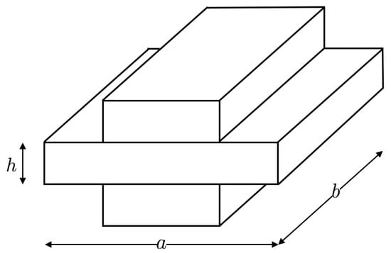
Figure 1.
Unit cell for a simple stiffened beam.
Here, the unit cell length (a), and the width (b), is 0.03 m. The non-stiffened beam base is 0.006 m thick, i.e., h is 0.006 m. The stiffeners are designed to be on both sides of the base beam and have the same width (b) and thickness (h). The dimension of the stiffener along the length of the unit cell is . Then, the unit cell is repeated to create the perfectly periodic beam where all the stiffeners are equally spaced. We achieve aperiodicity by keeping the dimensions of the stiffeners constant, while modulating the location of their center point according to the expression [4]:
where is the index number of the stiffener. Each location is projected from a circle of radius R, with parameter denoting a projection parameter (Figure 2).
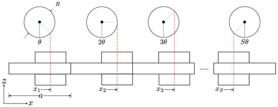
Figure 2.
Schematic of a quasiperiodically stiffened 3-D beam through projections from a circle.
To satisfy kinematic constraints for this stiffened beam, the radius of the circle is constrained to , in order to avoid an overlap of stiffeners in the resulting design. The pattern is studied by varying the projection parameter . For all the rational values of the projection parameter , we obtain a periodic beam with a periodic occurrence of a unit cell, or set of unit cells; however, all irrational values of identify a quasiperiodic arrangement of the stiffeners in a beam with no spatial translational symmetry. A common approach is to approximate the fractal frequency spectrum for all the real values of the projection parameter by considering rational values for and obtain the frequencies of a finite system with a large number of unit cells [4,41].
2.1. The Periodic Case: Unit Cell Analysis
To identify the vibration characteristics of the quasiperiodic beam, we first illustrate the dispersion behavior of a unit cell (Figure 1), which helps identifying bulk bandgaps shown in Figure 3. This analysis relies on a modal analysis that employs 3-D finite element analysis in COMSOL to find eigenfrequencies of the unit cell sweeping over a range of the wavenumber . The two end faces along the x-direction (dimension a) in Figure 1 are subjected to Bloch–Floquet periodic boundary conditions such that
where U, V, and W are the average displacements on the given faces of the unit cell in x, y, and z-directions, respectively. Here, the dispersion curves associated with all the modes such as bending, longitudinal, torsion, and other coupled modes are present. The polarization of these modes with contributions from the out-of-plane bending mode in Figure 3a and the in-plane bending mode in Figure 3b is illustrated with the goal of distinguishing the various branches for various modes of deformation i.e., out-of-plane bending mode, in-plane bending, longitudinal, torsional, and other coupled modes (in Figure 3c–i). The color in the dispersion curve, Figure 3a, represents the following out-of-plane bending mode polarization () given by
where u, v, and w are the averaged displacements over all the nodes in the 3-D model of the unit cell in x, y, and z-directions, respectively. Thus, the red color indicates the dominance of out-of-plane bending mode as opposed to the other modes in Figure 3a.
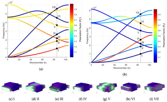
Figure 3.
(a) dispersion behavior of the unit cell polarized to the out-of-plane bending mode, i.e., stronger red color represents the more contribution from the out-of-plane bending mode; (b) dispersion behavior of the unit cell polarized to the in-plane bending mode, i.e., red color represents in-plane bending mode. Figures (c–i) are the mode shapes of the unit cell for the respective branch. Purple–white–green colormap is used to represent the deformation in the mode shapes with green representing the lowest and purple representing the height amplitude of deformation. Roman numerals I–VII are used to label the modes such that (c) I—out-of-plane bending (first), (d) II—torsion (first), (e) III—out-of-plane bending (second), (f) IV—in-plane bending (first), (g) V—torsion (second), (h) VI—in-plane bending (second), (i) VII—axial (first).
Similarly, the polarization factors for the other modes such as the in-plane bending mode () can be evaluated using Equation (4) and plotted on the dispersion curves, as shown in Figure 3b:
In Figure 3, the first out-of-plane bending and the first in-plane bending branch associated with the first bending mode of either kind can be identified by a polarization factor of value 0.85 or higher. The value of for the second out-of-plane bending mode is higher at low frequencies, but it decreases at higher values of frequency. The first torsional branch can be identified in its entirety from the in-plane bending polarization factor by having .
It is evident from the color scheme in the polarized dispersion curves shown in Figure 3 that, with an increase in frequency values, the polarization factor for the chosen mode reduces in value. This shows that, in 3-D, the higher-order modes associated with the corresponding degree of freedom are coupled with the modes of the other degrees of freedom. 3-D modeling of the unit cell results in a more complex dispersion behavior as compared to the reduced-order beam modeling of the unit cells in bending [4,5,37,42] as reduced-order beam model would only contain the information about the beam modes represented by the degrees of freedom chosen in the beam model. This is why, in Section 2.2, we plot the bulk spectrum of the 3-D quasiperiodic beams mostly in the range of the first branch of the dispersion curve, except for the out-of-plane bending mode which is studied experimentally for a finite beam over a wide range of frequencies in Section 2.3.
Once the branches of the respective modes are identified, the corresponding polarizations are used in mode identification when solving for long finite structures, thus leading to a frequency spectrum for the desired mode type. This spectrum could then be used to identify bandgaps in the bulk spectrum of infinitely long structures, localized modes at the edges or interfaces in the finite beams, and detailed dynamic behavior of such stiffened structures.
2.2. Spectral Properties—Bulk and Finite Domains
Next, we investigate the vibration characteristics of the quasiperiodic beams. We evaluate the spectral properties of infinite beams as a function of the projection parameter by discretizing its range in steps , which leads to an infinitely dense subset of as . In this framework, the bulk spectrum is computed for the discretization of the parameter space that identifies all commensurate/periodic rings defined by the rational values of whose vibrational spectrum approximates the bulk spectrum evaluated for all . We set and evaluate eigenfrequencies for unit cells to which we apply periodic boundary conditions.
The black dots in Figure 4a correspond to the computed eigenfrequencies, while the bandgaps are identified by white regions. No clear gaps are observed, as the space is filled by several overlapping gaps produced by the multiple mode polarizations. Clearer patterns can be identified by applying the polarization factor, as described in Equation (3) and color-coding the bulk spectrum as shown in Figure 4b. From this representation, it is clear that each mode has its own Hofstadter butterfly spectrum, and that the polarization parameter helps in separating eigenfrequencies associated with respective modes and in aiding the process of plotting them separately as done in Figure 5a,d,g. In the figures, we observe the presence of a bandgap for which we refer to as trivial bandgap, as it is present in the periodic beam and it is largely unaffected by the changes in the value of the projection parameter . With an increase in the value of , the bulk spectrum splits into a number of smaller non-trivial gaps whose location varies for the different modes.
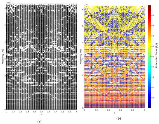
Figure 4.
Bulk frequency spectrum for all beam modes. (a) raw frequency spectrum; (b) frequency spectrum polarized with polarization factor , revealing butterflies associated with various modes.
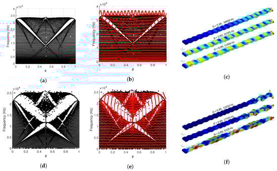
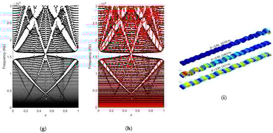
Figure 5.
For the first in-plane bending mode, (a–c) represent the bulk spectrum obtained from a commensurate structure of 100 unit cells, finite spectrum (in red) of the cantilever beam made of 20 unit cells overlapped with the the bulk spectrum (in black), and the representative mode shapes for given frequencies and , respectively. Similar information is provided for the first torsional mode in (d–f) as well as the out-of-plane bending modes in (g–i).
Furthermore, we investigate the spectrum of finite beams consisting of 20 unit cells i.e., . The eigenfrequencies for fixed-free (cantilever) beams are evaluated by considering the same discretization of used for the bulk spectrum. As expected by results from prior work [4], the finite spectrum of finite beams is characterized by eigenfrequencies that span the bulk bandgaps as shown in Figure 5b,e,h. Figure 5c,f,i illustrate the shape of specific modes of the finite spectrum that overlap with the bulk spectrum or with the non-trivial bandgaps that are formed due to the bifurcation of the bulk spectrum. It is seen that the modes close to the non-trivial bandgaps are localized at the edges.
The topological modes, such as the edge localized modes shown in Figure 5c,f,i, can be predicted by estimating the Integrated Density of States (IDS) for the system. The IDS as a function of the projection parameter for the Hofstadter butterflies associated with the first in-plane bending mode, first torsional mode, and the first out-of-plane bending mode are plotted in Figure 6a–c. The IDS is normalized with the number of modes spanning the first branch of the respective modes chosen. Figure 6d represents the IDS as a function of the eigenfrequencies with a sharp jump depicting the presence of a bandgap. This bandgap is essentially translated to the sharp jump in color levels of Figure 6a–c. These jumps in color level occur at an IDS level that varies linearly with respect to the projection parameter for a given topological or non-trivial bandgap. For trivial bandgap, the IDS value doesn’t change with the value of .
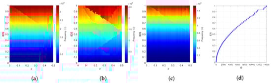
Figure 6.
(a–c) Integrated Density of States (IDS) as a function of exhibits a sharp jump in color level at the bandgaps for (a) first in-plane bending mode, (b) first torsional mode, and (c) first out-of-plane bending mode; (d) IDS for the out-of-plane bending mode at the projection parameter value of that is chosen in Section 2.3 for further theoretical and experimental studies.
Moreover, we also compute the numerical Frequency Response Function (FRF) of the cantilevered beam for different values of the projection parameter with a transverse harmonic excitation applied at the free end, i.e., at in order to excite the out-of-plane bending mode. The spatially averaged FRFs are shown in Figure 7b–d, where averages are respectively over the range of entire length (), , and . The colormap evolves from blue to red corresponding to the log scale of the magnitude of the FRF in dBs. A comparison of the numerical FRF for the out-of-plane bending mode with respect to the bulk and finite spectrum of the beam is presented in Figure 7. We observe how both bulk and finite structure gap resonances match the predictions from the spectral analysis reported for comparison in Figure 7a. We further note a higher spatially averaged magnitude of the frequency response of a region towards the free end of the beam (Figure 7d), where the excitation is applied, as compared to the spatially averaged magnitude of a region towards the root (Figure 7c). Thus, we infer that the modes associated with the eigenfrequencies of the finite quasiperiodic beams spanning the bandgaps in the bulk spectrum are the ones that are localized at the right boundary. This is further demonstrated in the next section by considering a finite beam with .
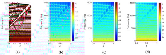
Figure 7.
Bulk (black dots) and finite (red dots) spectrum for the out-of-plane bending mode (a). FRFs in out-of-plane bending, spatially averaged over a portion of the beam length (b–d): (b), (c), and (d).
2.3. Experimental Results on a Finite Beam
For a comparison of the theoretical analysis with experiments, we choose a finite beam made of 20 unit cells, with the projection parameter that results in a design as shown in Figure 8a. The beam consisting of 20 unit cells is manufactured using an abrasive based water-jet cutter. The beam is excited in out-of-plane bending mode by an amplified burst chirp signal with a frequency range of 10–22 kHz using a ceramic disc-shaped piezoelectric actuator pasted close to the tip of the beam as shown in Figure 8b. Furthermore, the beam is subjected to cantilever conditions by using appropriate mounts as shown in Figure 8c. The frequency response of the beam is measured using the Polytec PSV-500 Xtra scanning laser Doppler vibrometer (supplied by Polytec Inc., Irvine, CA) over a grid of 750 points with five points along the width and 150 points along the beam length (from the clamped boundary at to the free end at ) corresponding to a spatial resolution of 4 mm in both directions.
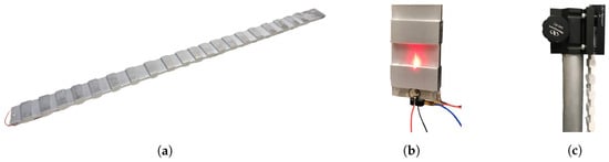
Figure 8.
Experimental set-up: (a) stiffened beam with parameter , (b) cantilever beam’s free end equipped with disc-shaped piezoelectric actuator, (c) mounts representing the cantilever boundary.
Figure 9 shows a comparison between the numerical results obtained from the 3-D FEM simulations (Figure 9a) and the results obtained from an experimental measurement of FRFs of the beam (Figure 9b). The numerically obtained FRFs for the finite beam is plotted in Figure 9a as a colormap where red color indicates a high amplitude of the response in dBs and blue indicates the lower extremes of the amplitude. The scales of the colorbar differ in Figure 9a,b due to the difference in the loads applied numerically and experimentally. The numerical and experimental FRFs for the desired out-of-plane bending mode appear to be slightly different due to the presence of large displacement amplitudes in experimentally obtained frequency response, in the region of numerically obtained bandgaps represented by dark blue bands in Figure 9a. This is likely caused by contamination of the experimental frequency response due to the unwanted excitation of the torsional mode which is possible due to a slight eccentricity of the actuator during manufacturing of the experimental set-up. Figure 10 demonstrates how the characteristics of the two modes overlap and even a slight coupling between them is undesirable. It is clear from Figure 10a that the bulk spectrum of the torsional mode overlaps with the non-trivial bandgap of the out-of-plane bending mode and vice versa with very small areas resulting in a complete bandgap when both of these modes are considered together. Here, the bulk spectrum of the torsional mode is represented in blue, and the bulk spectrum of the out-of-plane bending mode is represented in black. Similarly, finite torsional modes may also span the non-trivial and trivial bandgaps in the frequency spectrum of the out-of-plane bending modes as shown in Figure 10b justifying the presence of displacement amplitude in theoretical bandgap for the out-of-plane bending mode in the bulk of the finite beam made of 20 stiffeners.
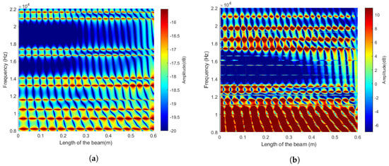
Figure 9.
FRF of the beam subject to tip harmonic excitation: (a) numerically obtained FRF; (b) experimentally obtained FRF.
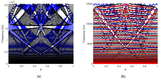
Figure 10.
(a) Overlapping bulk spectrum obtained from a commensurate structure of 100 unit cells for both torsional (blue) and out-of-plane bending (black) modes; (b) bulk spectrum of out-of-plane bending mode overlapped with the finite spectrum of cantilever beam made of 20 unit cells associated with the out-of-plane bending mode in red and the torsional mode in blue.
These differences in the numerical and experimental FRF and the presented arguments are further studied by comparing the nature of the bulk and finite spectrum of the stiffened beam with the experimental response of the finite beam as shown in Figure 11. For this, a portion of the bulk and finite spectrum for out-of-plane bending mode, obtained with the numerical method presented in Section 2.2, is plotted in Figure 11a. The plot consists of a wider bandgap associated with the first out-of-plane bending mode, the bandgap between the first and second out-of-plane bending mode, and the bandgap in the second out-of-plane bending mode. Here, the value of the projection parameter as 0.89 is also marked with a solid blue line. As mentioned in the Section 2.2, we would primarily focus on the bandgaps associated with the first branch of the respective modes only. Thus, the two evident bandgaps are identified between 11.46–12.95 kHz and 13.9–16.42 kHz represented by red and blue, respectively. For direct comparison, these bandgaps are plotted on top of the experimental frequency response for the indicated span-wise locations in Figure 11b–d.
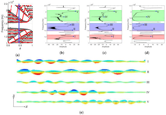
Figure 11.
(a) Numerical results with solid blue line representing case with ; (b–d) experimental frequency response for the case with at the spatial location: (b) 0.20L; (c) 0.25L; (d) averaged over the range. The red and green regions represent the numerically obtained non-trivial bandgap, whereas the blue region represents the trivial bandgap. (e) Experimentally obtained mode shapes for the peaks in the experimental frequency response plots lying in the theoretical bandgaps are actually the torsional modes due to contamination of the out-of-plane bending mode’s frequency response. The points shown are the locations of the experimentally obtained wavefield data. A jet colormap is overlapped with the deformation to provide a reference.
The experimental FRF has definitive peaks (represented with solid blue dots and roman numerals I–VII) visible within the theoretically estimated bandgaps for out-of-plane bending modes. This is evidence of a significant dynamic response of the beam at those frequencies. Upon further investigation of the experimental modes shapes of the finite beam by plotting the experimentally obtained full-filed data at those frequencies in Figure 11e, it is observed that all of those experimental resonant modes contributing to the dynamics of the finite beam are torsional modes, thus leading to a conclusion that the experimental frequency response values are contaminated by the unintentional excitation of torsional modes due to a point source for the excitation shown in Figure 8b. In addition, the peak in the frequency response close to 18 kHz is identified as a finite torsional mode shown in Figure 5e that is spanning the bandgap in the bulk spectrum of the first torsional branch. This mode is observed to be localized at the free edge which is also the location of the excitation. This overall qualitative comparison demonstrates that the experimental results are in direct correlation to the numerical results evaluated earlier.
3. Sandwich Quasiperiodic Beams
Sandwich structures consist of two stiff skin panels bonded to a lightweight core. An impedance mismatch is introduced to obtain the bandgaps in the frequency spectrum by alternating the core material. The two alternating core materials are the regular hexagonal honeycomb core and the re-entrant (auxetic) honeycomb core as shown in Figure 12, thus creating a periodic arrangement of the two distinct core materials [43]. In this work, quasiperiodic arrangements of the alternating core materials are obtained, and their frequency spectrum is studied with respect to a projection parameter similar to the one chosen for the stiffened beam in Section 2.2.
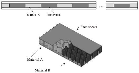
Figure 12.
Schematic of a sandwich beam’s alternating core.
3.1. Dynamics of Sandwich Beams
To study the behavior of quasiperiodic beams, it is important to theoretically model such composite phononic crystals. With a similar approach as described in Ref. [43], we first compute the governing equations with the help of Hamilton’s principle. Then, the governing equations are transformed into a transfer matrix formulation to obtain the transfer matrix of the chosen unit cell. Then, the transfer matrix is used to obtain the dynamic stiffness matrix of the unit cell that is further used to obtain the global dynamic stiffness matrix of the phononic crystal. Finally, the FRF for the quasiperiodic sandwich beams is computed for a chosen distribution of projection parameter using the global dynamic stiffness matrix.
3.1.1. Geometric and Material Properties
For modeling the phononic crystal as a sandwich beam, the chosen unit cell, as shown in Figure 13, is comprised of three portions where the core of length , at the two extreme positions, is made of the regular honeycomb, i.e., material A, while the core of the middle portion is made of the auxetic honeycomb, i.e., material B. Within each of these portions, the sandwich beam is uniform and doesn’t have any span-wise heterogeneity. Furthermore, we obtain a periodic arrangement of these unit cells leading to a basic periodic phononic crystal. Then, we introduce quasiperiodicity like we did in Section 2 for the stiffened beam by keeping the dimensions of the auxetic core (material B) constant, while modulating the location of their center point according to the expression in Equation (1). The phononic crystals resulting from the quasiperiodic arrangement of the auxetic honeycomb core with respect to the regular honeycomb core are shown in Figure 14.
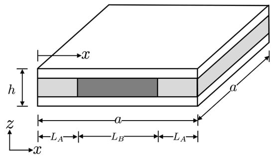
Figure 13.
Geometry of the unit cell.
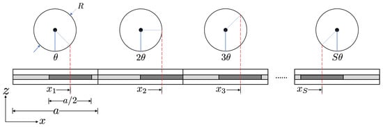
Figure 14.
Schematic of a quasiperiodic sandwich beam through projections from a circle.
As far as the material properties are concerned, we derive the properties from Ref. [43]. The face sheets are made of elastic and isotropic material, i.e., aluminum. In analyzing the behavior of sandwich beams, the assumption is that the face sheets undergo only longitudinal strain, i.e., they do not undergo any shear deformation in transverse directions. We neglect the normal strains in the core and keep the terms associated with only the shear strains due to a low shear modulus of the core as compared to the face sheets [44]. The core is made of material called Nomex, whose mechanical properties are described in Ref. [45], i.e., = 900 MPa, = 0.4 and = 724 kg/m3. Using the work of Gibson and Ashby [46], the shear modulus for the regular honeycomb (material A) is obtained to be MPa and density kg/m3 as opposed to the shear modulus of the auxetic core (material B) whose MPa and kg/m3. Furthermore, the distributed parameter model to analyze the behavior of such sandwich structures is also taken from Ruzzene et al. [43].
3.1.2. Harmonic Response
To evaluate the harmonic response, we first evaluate the transfer matrix of the unit cell and then recast it into a suitable dynamic stiffness matrix as mentioned above. The key difference in the methodology presented in this work as compared to Ref. [43] is the geometry of the unit cell (Figure 13) leading to a change in the definition of state vectors at the extremes of each portion forming the unit cell. Thus, a suitably modified formulation accounting for the three portions of the unit cell is employed in this work. Transfer matrix of the unit cell, , can be obtained by multiplying the transfer matrices of the three portions composite the entire unit cell such that
where and denote the transfer matrices for the portions of the beam with material A and material B, respectively. The eigenvalues of enable the identification of bandgaps in the frequency spectrum for different configurations of the sandwich beam. These eigenvalues of the matrix can be obtained by solving the following eigenvalue problem ([47,48,49]):
where represents the state vector of generalized displacements and forces of the sandwich beam at the beginning or the left end. Furthermore, the state vectors, , at the beginning and the end of the sandwich beam can be related through the eigenvalues of the transfer matrix that determine the nature of wave dynamics along the structure as shown in Equation (7)
Waves are free to propagate along the beam for those values of frequency that make , whereas, if , waves are attenuated. The eigenvalue can also be rewritten as ([47,50])
where is a frequency dependent parameter called the wavenumber used in Section 2. The real part of represents the decay of the amplitude of a wave propagating from one end of the beam to the other end and the imaginary part of determines the phase change. Wave propagation is therefore possible within the frequency bands where is purely imaginary (bulk region), while the attenuation occurs for those values of frequency that provide a real part to the propagation constant (bandgap). Hence, the real and imaginary parts of the propagation constant as well as the eigenvalues of the transfer matrix define frequency bands where energy is transmitted or attenuated along the beam length. This method of obtaining the pass and stop frequency bands yields results similar to the dispersion curves for unit cells, studied in Section 2.
Subsequently, to obtain a dynamic stiffness matrix of the cell, Equation (7) can be expanded as follows:
where and represent the generalized displacements and forces at the left ’L’ and right ’R’ cell boundaries, denoted by the subscripts, while are partitions of the cell transfer matrix . For the transformation, Equation (9) can be rearranged so that the generalized forces at the cell ends are related to the generalized displacements to obtain:
where [] represents the dynamic stiffness matrix for the unit cell of the periodic sandwich beam such that
Rearranging terms in the equation above yields
Finally, the equation using the dynamics stiffness matrix can be written as
Equation (16) represents the dynamic behavior of a unit cell of the considered periodic sandwich beam, where represents the dynamic stiffness matrix of the unit cell.
As opposed to the traditional FEM, however, this dynamic stiffness matrix is obtained from the exact solution of the equation of motion for the beam. The resulting model replicates the exact displacement distributions over the entire structural member and thus allows for using a significantly reduced number of elements than conventional FEM, similar to the spectral finite element technique ([51,52,53,54]). However, the approach to solving for the entire periodic sandwich beam as shown in Figure 12 as well as its quasiperiodic configurations shown in Figure 14 involve assembling a global dynamic stiffness matrix from the dynamic stiffness matrix of individual cells forming the entire beam using standard procedure applied in conventional FEM. The analysis of quasiperiodic configurations of the sandwich beam is described in the next section.
3.2. Numerical Results: Frequency Response Function
The harmonic transverse response of periodic and quasiperiodic placement of the alternating core material subjected to the beam’s base excitation is studied in this section. The total beam length is taken to be 2 m. The length of each unit cell is 0.1 m and the width is 0.04 m. The total thickness of the sandwich beam is 0.004 m with the thickness of each face sheet to be 0.001 m. The length of the portion of the auxetic core is fixed to be 0.05 m. Once a quasiperiodic arrangement is obtained based on the location of the auxetic core, the remaining core is filled with the regular hexagonal core material. Furthermore, the sandwich beam’s base or the left end () is excited by a vertical harmonic motion with frequencies varying between 0 and 1600 Hz. This is done for a set of periodic beams that are obtained with the projection parameter belonging to a set of rational numbers to estimate the behavior of quasiperiodic beams that are governed by irrational values of the projection parameter. Figure 15 demonstrates a periodic sandwich beam’s deformation where the projection parameter is chosen to be zero, i.e., , and the base is excited with the frequencies of 300, 600, and 900 Hz. It is evident from Figure 15b that the energy is localized at the left end when the sandwich beam is excited at 600 Hz, depicting the presence of the trivial bandgap.
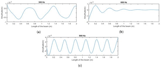
Figure 15.
Numerically obtained deformed shapes of the periodic sandwich beam at frequencies: (a) 300 Hz, (b) 600 Hz, and (c) 900 Hz.
Finally, the FRF corresponding to the vertical displacement of the beam’s middle node and the tip for the family of beams are plotted in Figure 16a,b, respectively. Figure 16 indicates the presence of frequency bands where the response of the beam is highly attenuated. The frequency bands for the periodic sandwich beam correspond to the stop bands obtained from the dispersion curves of the unit cell. Finally, for the FRF, when plotted with respect to the projection parameter (), the frequency bands exhibit the well-known Hofstadter’s butterfly.
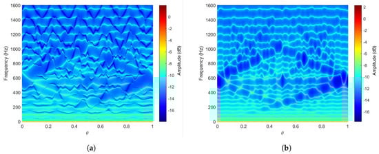
Figure 16.
Numerical frequency-response function using dynamic stiffness matrix under base excitation while the response is evaluated at (a) middle node, (b) tip of the sandwich beam.
4. Conclusions
In this paper, we study the dynamic behavior of quasiperiodic structural beams built with two distinct characteristics. A family of such beams is generated by varying a projection parameter defining the location of distinct characteristics, such as stiffeners locations and core mechanical properties. We first consider a stiffened isotropic beam that resembles a stepped beam, which is characterized by a trivial bandgap in the case of the periodic beam. We subsequently identify additional non-trivial bandgaps by computing the bulk spectrum. This involves a process of characterizing the modes in the bulk spectrum by evaluating the corresponding polarization factors. We observe non-trivial bandgaps appearing in the form of the well-known Hofstadter butterfly. Next, the spectrum of finite structures in the form of a cantilever beam with 20 unit cells is studied and compared with the bulk spectrum. We observe resonant modes spanning the non-trivial bandgaps which are found to be localized at the right boundary from the calculation of mode shapes. This is verified numerically and experimentally by the FRF obtained by exciting only the out-of-plane bending mode for the family of quasiperiodic beams and a stiffened beam manufactured with a particular value of .
Secondly, we consider sandwich beams with alternating core material where the location of the auxetic honeycomb core is determined from the function that leads to the family of periodic and quasiperiodic beams. Due to the kinematic assumptions involved in the analysis of such beams, a dedicated model is developed that leads to a suitable dynamic stiffness matrix for the phononic crystals for the evaluation of the FRF in the chosen out-of-plane bending mode. Thus, the bandgaps can be identified from the fractal spectra obtained using the numerical FRF.
In conclusion, the study demonstrates the occurrence of bandgaps in the frequency spectrum of 1D continuous quasiperiodic elastic media resulting from a discontinuity in the geometric or material property repeated over the length of the elastic media while the location of the discontinuity is varied. These bandgaps can be leveraged towards the self-attenuating designs of beams or locally resonant beam structures.
Author Contributions
Conceptualization, M.R.; methodology, M.G., and M.R.; software, M.G.; validation, M.G.; formal analysis, M.G.; investigation, M.G., and M.R.; resources, M.R.; data curation, M.G.; writing—original draft preparation, M.G.; writing—review and editing, M.R.; visualization, M.G.; supervision, M.R.; project administration, M.R.; funding acquisition, M.R. All authors have read and agreed to the published version of the manuscript.
Funding
This research received no external funding.
Conflicts of Interest
The authors declare no conflict of interest.
Abbreviations
The following abbreviations are used in this manuscript:
| 3-D | Three-dimensional |
| FEM | Finite Element Method |
| FRF | Frequency Response Function |
| IDS | Integrated Density of States |
| QP | Quasi-Periodic |
References
- Süsstrunk, R.; Huber, S.D. Observation of phononic helical edge states in a mechanical topological insulator. Science 2015, 349, 47–50. [Google Scholar] [CrossRef] [PubMed]
- Mousavi, S.H.; Khanikaev, A.B.; Wang, Z. Topologically protected elastic waves in phononic metamaterials. Nat. Commun. 2015, 6, 8682. [Google Scholar] [CrossRef] [PubMed]
- Anderson, P.W. Absence of diffusion in certain random lattices. Phys. Rev. 1958, 109, 1492. [Google Scholar] [CrossRef]
- Pal, R.K.; Rosa, M.I.N.; Ruzzene, M. Topological bands and localized vibration modes in quasiperiodic beams. New J. Phys. 2019, 21, 093017. [Google Scholar] [CrossRef]
- Xia, Y.; Erturk, A.; Ruzzene, M. Topological edge states in quasiperiodic locally resonant metastructures. Phys. Rev. Appl. 2020, 13, 014023. [Google Scholar] [CrossRef]
- Chaplain, G.; Makwana, M.; Craster, R. Rayleigh–Bloch, topological edge and interface waves for structured elastic plates. Wave Motion 2019, 86, 162–174. [Google Scholar] [CrossRef]
- Hodges, C.; Woodhouse, J. Confinement of vibration by structural irregularity. J. Acoust. Soc. Am. 1981, 69, S109. [Google Scholar] [CrossRef]
- Hodges, C. Confinement of vibration by structural irregularity. J. Sound Vib. 1982, 82, 411–424. [Google Scholar] [CrossRef]
- Sievers, A.; Takeno, S. Intrinsic localized modes in anharmonic crystals. Phys. Rev. Lett. 1988, 61, 970. [Google Scholar] [CrossRef]
- Page, J. Asymptotic solutions for localized vibrational modes in strongly anharmonic periodic systems. Phys. Rev. B 1990, 41, 7835. [Google Scholar] [CrossRef]
- Sheng, P. Scattering and Localization of Classical Waves in Random Media; World Scientific: Singapore, 1990; Volume 8. [Google Scholar]
- Photiadis, D.M.; Houston, B.H. Anderson localization of vibration on a framed cylindrical shell. J. Acoust. Soc. Am. 1999, 106, 1377–1391. [Google Scholar] [CrossRef]
- Campbell, D.K.; Flach, S.; Kivshar, Y.S. Localizing energy through nonlinearity and discreteness. Phys. Today 2004, 57, 43–49. [Google Scholar] [CrossRef]
- Hu, H.; Strybulevych, A.; Page, J.; Skipetrov, S.E.; van Tiggelen, B.A. Localization of ultrasound in a three-dimensional elastic network. Nat. Phys. 2008, 4, 945–948. [Google Scholar] [CrossRef]
- Han, P.; Chan, C.; Zhang, Z. Wave localization in one-dimensional random structures composed of single-negative metamaterials. Phys. Rev. B 2008, 77, 115332. [Google Scholar] [CrossRef]
- Prodan, E.; Prodan, C. Topological phonon modes and their role in dynamic instability of microtubules. Phys. Rev. Lett. 2009, 103, 248101. [Google Scholar] [CrossRef]
- Nash, L.M.; Kleckner, D.; Read, A.; Vitelli, V.; Turner, A.M.; Irvine, W.T. Topological mechanics of gyroscopic metamaterials. Proc. Natl. Acad. Sci. USA 2015, 112, 14495–14500. [Google Scholar] [CrossRef]
- Chen, H.; Yao, L.; Nassar, H.; Huang, G. Mechanical quantum hall effect in time-modulated elastic materials. Phys. Rev. Appl. 2019, 11, 044029. [Google Scholar] [CrossRef]
- Pal, R.K.; Schaeffer, M.; Ruzzene, M. Helical edge states and topological phase transitions in phononic systems using bi-layered lattices. J. Appl. Phys. 2016, 119, 084305. [Google Scholar] [CrossRef]
- Chen, H.; Nassar, H.; Norris, A.N.; Hu, G.; Huang, G. Elastic quantum spin Hall effect in kagome lattices. Phys. Rev. B 2018, 98, 094302. [Google Scholar] [CrossRef]
- Vila, J.; Pal, R.K.; Ruzzene, M. Observation of topological valley modes in an elastic hexagonal lattice. Phys. Rev. B 2017, 96, 134307. [Google Scholar] [CrossRef]
- Liu, T.W.; Semperlotti, F. Tunable acoustic valley–hall edge states in reconfigurable phononic elastic waveguides. Phys. Rev. Appl. 2018, 9, 014001. [Google Scholar] [CrossRef]
- Ozawa, T.; Price, H.M.; Goldman, N.; Zilberberg, O.; Carusotto, I. Synthetic dimensions in integrated photonics: From optical isolation to four-dimensional quantum Hall physics. Phys. Rev. A 2016, 93, 043827. [Google Scholar] [CrossRef]
- Kraus, Y.E.; Zilberberg, O. Quasiperiodicity and topology transcend dimensions. Nat. Phys. 2016, 12, 624. [Google Scholar] [CrossRef]
- Lahini, Y.; Pugatch, R.; Pozzi, F.; Sorel, M.; Morandotti, R.; Davidson, N.; Silberberg, Y. Observation of a localization transition in quasiperiodic photonic lattices. Phys. Rev. Lett. 2009, 103, 013901. [Google Scholar] [CrossRef]
- Vyunishev, A.M.; Pankin, P.S.; Svyakhovskiy, S.E.; Timofeev, I.V.; Vetrov, S.Y. Quasiperiodic one-dimensional photonic crystals with adjustable multiple photonic bandgaps. Opt. Lett. 2017, 42, 3602–3605. [Google Scholar] [CrossRef]
- Araújo, C.; Vasconcelos, M.S.; Mauriz, P.W.; Albuquerque, E.L. Omnidirectional band gaps in quasiperiodic photonic crystals in the THz region. Opt. Mater. 2012, 35, 18–24. [Google Scholar] [CrossRef]
- Bellingeri, M.; Chiasera, A.; Kriegel, I.; Scotognella, F. Optical properties of periodic, quasi-periodic, and disordered one-dimensional photonic structures. Opt. Mater. 2017, 72, 403–421. [Google Scholar] [CrossRef]
- Jin, C.; Cheng, B.; Man, B.; Li, Z.; Zhang, D.; Ban, S.; Sun, B. Band gap and wave guiding effect in a quasiperiodic photonic crystal. Appl. Phys. Lett. 1999, 75, 1848–1850. [Google Scholar] [CrossRef]
- Biancalana, F. All-optical diode action with quasiperiodic photonic crystals. J. Appl. Phys. 2008, 104, 093113. [Google Scholar] [CrossRef]
- Kraus, Y.E.; Lahini, Y.; Ringel, Z.; Verbin, M.; Zilberberg, O. Topological states and adiabatic pumping in quasicrystals. Phys. Rev. Lett. 2012, 109, 106402. [Google Scholar] [CrossRef]
- Apigo, D.J.; Qian, K.; Prodan, C.; Prodan, E. Topological edge modes by smart patterning. Phys. Rev. Mater. 2018, 2, 124203. [Google Scholar] [CrossRef]
- Dean, C.R.; Wang, L.; Maher, P.; Forsythe, C.; Ghahari, F.; Gao, Y.; Katoch, J.; Ishigami, M.; Moon, P.; Koshino, M.; et al. Hofstadter’s butterfly and the fractal quantum Hall effect in moiré superlattices. Nature 2013, 497, 598–602. [Google Scholar] [CrossRef]
- Yu, D.; Liu, Y.; Zhao, H.; Wang, G.; Qiu, J. Flexural vibration band gaps in Euler-Bernoulli beams with locally resonant structures with two degrees of freedom. Phys. Rev. B 2006, 73, 064301. [Google Scholar] [CrossRef]
- Süsstrunk, R.; Huber, S.D. Classification of topological phonons in linear mechanical metamaterials. Proc. Natl. Acad. Sci. USA 2016, 113, E4767–E4775. [Google Scholar] [CrossRef]
- Hofstadter, D.R. Energy levels and wave functions of Bloch electrons in rational and irrational magnetic fields. Phys. Rev. B 1976, 14, 2239. [Google Scholar] [CrossRef]
- Apigo, D.J.; Cheng, W.; Dobiszewski, K.F.; Prodan, E.; Prodan, C. Observation of topological edge modes in a quasiperiodic acoustic waveguide. Phys. Rev. Lett. 2019, 122, 095501. [Google Scholar] [CrossRef]
- COMSOL Multiphysics®. Introduction to COMSOL Multiphysics®; COMSOL AB: Stockholm, Sweden, 2020; Volume 11. [Google Scholar]
- Pryor, R.W. Multiphysics Modeling Using COMSOL®: A First Principles Approach; Jones & Bartlett Learning: Burlington, MA, USA, 2009. [Google Scholar]
- Olsson III, R.H.; El-Kady, I. Microfabricated phononic crystal devices and applications. Meas. Sci. Technol. 2008, 20, 012002. [Google Scholar] [CrossRef]
- Prodan, E.; Shmalo, Y. The K-theoretic bulk-boundary principle for dynamically patterned resonators. J. Geom. Phys. 2019, 135, 135–171. [Google Scholar] [CrossRef]
- Yin, J.; Ruzzene, M.; Wen, J.; Yu, D.; Cai, L.; Yue, L. Band transition and topological interface modes in 1D elastic phononic crystals. Sci. Rep. 2018, 8, 6806. [Google Scholar] [CrossRef]
- Ruzzene, M.; Scarpa, F. Control of wave propagation in sandwich beams with auxetic core. J. Intell. Mater. Syst. Struct. 2003, 14, 443–453. [Google Scholar] [CrossRef]
- Mead, D.; Markus, S. The forced vibration of a three-layer, damped sandwich beam with arbitrary boundary conditions. J. Sound Vib. 1969, 10, 163–175. [Google Scholar] [CrossRef]
- Zhang, J.; Ashby, M. The out-of-plane properties of honeycombs. Int. J. Mech. Sci. 1992, 34, 475–489. [Google Scholar] [CrossRef]
- Gibson, L.J.; Ashby, M.F. Cellular Solids: Structure and Properties; Cambridge University Press: Cambridge, UK, 1999. [Google Scholar]
- Langley, R. On the modal density and energy flow characteristics of periodic structures. J. Sound Vib. 1994, 172, 491–511. [Google Scholar] [CrossRef]
- Lin, Y.K.; McDaniel, T. Dynamics of beam-type periodic structures. J. Eng. Ind. 1969, 91, 1133–1141. [Google Scholar] [CrossRef]
- Roy, A.K.; Plunkett, R. Wave attenuation in periodic structures. J. Sound Vib. 1986, 104, 395–410. [Google Scholar] [CrossRef]
- Mead, D. A general theory of harmonic wave propagation in linear periodic systems with multiple coupling. J. Sound Vib. 1973, 27, 235–260. [Google Scholar] [CrossRef]
- Doyle, J.F. Wave propagation in structures. In Wave Propagation in Structures; Springer: Berlin/Heidelberg, Germany, 1989; pp. 126–156. [Google Scholar]
- Doyle, J.; Farris, T. Spectrally formulated element for wave propagation in 3-D frame structures. Int. J. Anal. Exp. Modal Anal. 1990, 5, 223–237. [Google Scholar]
- Gopalakrishnan, S.; Doyle, J. Wave propagation in connected waveguides of varying cross-section. J. Sound Vib. 1994, 175, 347–363. [Google Scholar] [CrossRef]
- Baz, A. Spectral finite-element modeling of the longitudinal wave propagation in rods treated with active constrained layer damping. Smart Mater. Struct. 2000, 9, 372. [Google Scholar] [CrossRef]
Publisher’s Note: MDPI stays neutral with regard to jurisdictional claims in published maps and institutional affiliations. |
© 2020 by the authors. Licensee MDPI, Basel, Switzerland. This article is an open access article distributed under the terms and conditions of the Creative Commons Attribution (CC BY) license (http://creativecommons.org/licenses/by/4.0/).