Approximating Catalyst Effectiveness Factors with Reaction Rate Profiles

Abstract

A novel approximate solution for catalyst effectiveness factors is presented. It is based on carefully selected approximate reaction rate profiles, instead of typical assumption of composition profiles inside the catalyst. This formulation allows analytical solution of the approximate model, leading to a very simple iterative solution for effectiveness factor for general nonlinear reaction stoichiometry and arbitrary catalyst particle shape. The same model can be used with all practical Thiele modulus values, including multicomponent systems with inert compounds. Furthermore, the correct formulation of the underlying physical model equation is discussed. It is shown that an incorrect but often-used model formulation where convective mass transfer has been neglected may lead to much higher errors than the present approximation. Even with a correctly formulated physical model, rigorous discretization of the catalyst particle volume may have unexpectedly high numerical errors, even exceeding those with the present approximate solution. The proposed approximate solution was tested with a number of examples. The first was an equimolar reaction with first order kinetics, for which analytical solutions are available for the standard catalyst particle geometries (slab, long cylinder, and sphere). Then, the method was tested with a second order reaction in three cases: (1) with one pure reactant, (2) with inert present, and (3) with two reactants and non-stoichiometric surface concentrations. Finally, the method was tested with an industrially relevant catalytic toluene hydrogenation including Maxwell-Stefan formulation for the diffusion fluxes. In all the tested systems, the results were practically identical when compared to the analytical solutions or rigorous finite volume solution of the same problem.

1. Introduction

Calculation of effectiveness factors for catalyst particles is one of the most classical problems in Chemical Reaction Engineering [1,2,3,4]. It combines reaction kinetics with transport phenomena in a nonlinear manner, making the solution far from trivial [5,6,7]. On one hand, catalyst development aims towards increasingly active catalysts, but on the other hand, relatively large catalyst particles are desired to minimize pressure drop in fixed beds or enhance catalyst separation in slurry reactors. These two desires lead to situations, where reaction rates near catalyst surface will be very different from that inside the particles. Therefore, it cannot be foreseen that this problem loses its importance.

Numerical solution of precise composition and reaction rate profiles in catalyst particles is in principle rather straightforward with current computational resources, even when combined with full reactor models [8], although calculation of effectiveness factors with very high precision is more challenging than often appreciated. When combined with identification of reaction kinetic parameters, process flowsheet optimization, or model based process control, computational effort becomes an important issue. There are always competing interests for increasing process model sophistication. Whenever the full process model can be solved with sufficient accuracy but with reduced computational effort, more details can be included elsewhere to improve the overall predictive power of the model.

Although mutual interactions between diffusion and reaction are traditionally addressed, another mass transfer mechanism, namely convection, is more often than not forgotten from the problem formulation, although its importance has been addressed in some very classical textbooks and publications [1,4,9]. Moreover, most of the numerical approximations found from the literature were based on physical models neglecting convective mass transfer [10,11,12,13,14,15,16,17]. This leads to a situation where the resulting error is not only due to mathematical approximation of the underlying differential equation (which is typically minimized by elegant mathematical manipulations), but in the reaction-diffusion model itself, which does not take into account all the relevant physical phenomena. The latter error can be much higher than the numerical approximation error.

In the classical numerical solutions found in the literature, the reaction rate is usually considered to depend on the concentration of one component only. Furthermore, these solutions are often kinetics-dependent, i.e., the order of reaction needs to be explicitly stated before applying the method [7,10,18]. However, in reactive systems, the component concentrations are heavily coupled due to the reactions, and usually, these systems cannot be properly described without considering every chemical component simultaneously. Many reactions catalyzed by a solid surface also follow reaction kinetics without a clear reaction order, such as the Langmuir-Hinshelwood model.

In this contribution, a novel method for effectiveness factor prediction is proposed. It is based on assumed reaction rate profiles instead of traditional composition profile approach used in most high-order numerical methods [5,7]. This novel approach allows analytical solution of the approximate problem, and with a carefully selected reaction rate profile, effectiveness factor predictions with comparable or in some cases even higher accuracy than much more rigorous numerical composition profile solutions. The proposed method is equally suitable for any reaction rate regime, catalyst shape, and reaction stoichiometry.

2. Model Development

Mathematically, material balances within catalyst particles can be modeled with the following reaction-diffusion-convection (RDC) Equation:

$$\frac{\partial \left(\mathrm{c}\right)}{\partial \mathrm{t}}=-\frac{1}{{\mathrm{r}}^{\mathrm{m}}}\frac{\partial }{\partial \mathrm{r}}\left({\mathrm{r}}^{\mathrm{m}}\left(\mathrm{N}\right)\right)+\left(\mathrm{R}\right)$$

(1)

where the parameter m is a geometry factor which takes value 0 for slab, 1 for cylindrical, and 2 for spherical geometry. The geometry factor can be generalized for other non-standard particle shapes as proposed by [19,20]. See also [21] for analysis of commercial catalyst shapes. The shape parameter can be estimated from:

$$\mathrm{m}=\mathrm{L}\frac{\mathrm{A}}{\mathrm{V}}-1$$

(2)

where L is the characteristic length for the chosen geometry. This is the slab half thickness, the cylinder radius, or the sphere radius for slab, cylindrical, and spherical geometry, respectively. A is the catalyst particle surface area and V is its volume. Non-integer values may also be used for other than standard geometries. A reasonable approximation may be obtained if the A/V ratio of a non-standard geometry is used along with the smallest half thickness for L. [20,22,23].

Boundary conditions for the reaction-diffusion-convection model are symmetrical at the center (∂/∂r = 0 at r = 0) and known catalyst surface compositions (c = c_L at r = L). Additionally, an obvious requirement is that the solutions are finite everywhere [2].

In this contribution, we were interested in steady state solutions, and time derivatives were set to zero. Typically, the time scales for composition profile development are much faster than other relevant time scales in the reactors, except in some rare cases, such as when analyzing particle scale origins of detrimental reaction runaway [24].

The mass transfer flux (relative to external reference coordinates) consists of diffusive flux (relative to molar average velocity frame) and convective flux. The mass transfer flux can be written in the following way:

$$\left(\mathrm{N}\right)=-{\mathrm{c}}_{\mathrm{t}}\left[\mathrm{D}\right]\frac{\partial \left(\mathrm{x}\right)}{\partial \mathrm{r}}+{\mathrm{N}}_{\mathrm{t}}\left(\mathrm{x}\right)$$

(3)

The first part on the right hand side describes diffusive and the second convective flux. N_t is the sum of all individual mass transfer fluxes. For the diffusive part, there are also alternative formulations besides the mole fraction gradient for the driving force. These could be incorporated in the present model, but were left out here to avoid excessive complications in the model derivation [25]. Convective flux within the pores typically originates from pressure gradients caused by non-equimolar reactions, and could be modeled, e.g., with the dusty gas model [1]. However, in cases with closed catalyst volumes, the pressure gradients were not easily determined and they were probably relatively low. Therefore, it was better to formulate the model in such a way that pressure gradients were assumed negligible, and the equation of state connecting molar volume, local compositions, temperature, and (constant) pressure was valid everywhere within the catalyst particle [26].

As is typical in the literature with diffusion inside porous catalyst particles, the diffusion coefficients were assumed to contain porosity and tortuosity effects as well as a constriction factor. The effect of surface diffusion could be included in the model in a similar manner if a reliable model was available for it. In case of very narrow pores, diffusion coefficients should be calculated based on Knudsen diffusion; otherwise, bulk fluid coefficients should be used [1,3]. One often-neglected restriction is that the diffusion fluxes must sum up to zero, as diffusion describes molecular movement with respect to the average molar flow. This limitation should be incorporated in the matrix if diffusion coefficients [D]. Unfortunately, with effective diffusion models, this limitation is typically violated [25,26].

When spatial derivatives of diffusion coefficients and total concentration are assumed negligible as compared to the other terms (corresponding to the linearized theory of mass transfer, or Toor-Stewart-Prober assumption), we end up with the following reaction-diffusion-convection equation:

$${\mathrm{c}}_{\mathrm{t}}\left[\mathrm{D}\right]\frac{{\partial }^2\left(\mathrm{x}\right)}{\partial {\mathrm{r}}^2}+{\mathrm{c}}_{\mathrm{t}}\left[\mathrm{D}\right]\frac{\mathrm{m}}{\mathrm{r}}\frac{\partial \left(\mathrm{x}\right)}{\partial \mathrm{r}}-\frac{\mathrm{m}}{\mathrm{r}}{\mathrm{N}}_{\mathrm{t}}\left(\mathrm{x}\right)-{\mathrm{N}}_{\mathrm{t}}\frac{\partial \left(\mathrm{x}\right)}{\partial \mathrm{r}}-\left(\mathrm{x}\right)\frac{\partial {\mathrm{N}}_{\mathrm{t}}}{\partial \mathrm{r}}=-\left(\mathrm{R}\right)$$

(4)

Reaction term (R) is an arbitrary function of compositions. It can also depend on other state variables such as temperature and pressure; however, since in this contribution they were assumed constant, their effect was assumed to be included in the reaction rate coefficients. Note that this RDC equation is specified for all but one component. The last component mole fraction profile is obtained from the obvious fact that the mole fractions sum up to unity.

2.1. Reaction Rate Profile Approximation

Classical numerical solutions to the reaction-diffusion equation are based on polynomial approximations for the composition profiles [5,7]. These solutions typically neglect convective part for mass transfer, which could be significant in case of non-equimolar reactions. From a mathematical point of view, erroneous numerical solution can be seen when mole fractions do not up to one, or when the solution is written in terms of component concentrations instead of mole fractions, the resolved concentrations within the catalyst particle do not satisfy the equation of state. The total flux at any point of the catalyst could be calculated by integrating reaction rates from the catalyst particle center up to that point. Another option is to solve the model so that total flux is calculated based on the requirement for mole fractions summing up to one. This transforms the model into algebraic-differential equation; however, since nonlinear reaction kinetics already calls for an iterative solution, this does not change the final nature of the equations to be solved. The third option is to calculate total flux explicitly based on diffusion fluxes of any of the reacting components and reaction stoichiometry; however, this approach easily leads to poorer convergence of the whole set of nonlinear equations although the number of iterated variables would be less.

In this contribution, the reaction rates were assumed to be of the following polynomial form:

(R) = R(c) = R(r) = (a) + (b)rⁿ

(5)

These rates are the true formation or consumption rates for each component (including stoichiometry), not reaction extent rates. Although the reaction rate expression is explicitly written based on the location instead of concentrations, parameters a, b, and n depend on concentrations; thus, the applied expression takes concentration dependency into account.

This functional form is quite flexible for approximate description of various reaction rate profiles found in practical situations. Nearly constant reaction rate profiles can be observed when the diffusional mass transfer compensates concentration changes caused by the reaction. Low values of parameter n describe these systems well, and the constant term (a) dominates the reaction rate profile. If the reaction rate is rapid compared to the diffusional mass transfer, the limiting reagent is consumed near the surface, leading to steep profiles also for the reaction rates. In these cases, parameter n is high, and the second term of the reaction rate profile approximation dominates. This may also be formulated so that constant reaction rate can be found in systems with low values of Thiele modulus, while steep reaction rate profiles can be found in systems with high values of Thiele modulus [4,9].

After assuming a profile for the reaction rate as a function of location (independent variable) instead of composition (dependent variable), the RDC model transforms into a linear differential equation also in cases of nonlinear reaction kinetics. This allows for an analytical solution. The remaining problem is to find the three unknown reaction rate profile parameters (a, b and n) in such a way that the reaction rate profile is as close as possible to the true solution. Parameter n is a single scalar specific to the reaction, and parameters a and b are vectors (scalars for each component).

For the simplified model, we made some further assumptions. The last three terms on the right hand side (the convection terms) are assumed spatially invariant:

$$\frac{\mathrm{m}}{\mathrm{r}}{\mathrm{N}}_{\mathrm{t}}\left(\mathrm{x}\right)\approx \frac{\mathrm{m}}{\mathrm{L}}{\mathrm{N}}_{\mathrm{t}\mathrm{c}}\left({\mathrm{x}}_{\mathrm{c}}\right)$$

(6)

$${\mathrm{N}}_{\mathrm{t}}\frac{\partial \left(\mathrm{x}\right)}{\partial \mathrm{r}}\approx \frac{\left(\mathrm{m}+1\right){\mathrm{N}}_{\mathrm{t}\mathrm{c}}}{\mathrm{L}}\left(\left({\mathrm{x}}_{\mathrm{L}}\right)-\left({\mathrm{x}}_0\right)\right)$$

(7)

$$\mathrm{x}\frac{\partial {\mathrm{N}}_{\mathrm{t}}}{\partial \mathrm{r}}\approx \frac{{\mathrm{N}}_{\mathrm{t}\mathrm{c}}}{\mathrm{L}}\left({\mathrm{x}}_{\mathrm{c}}\right)$$

(8)

where (x_c) is a vector of average convective mole fractions and N_tc is the average total flux for the convective term. Average convective mole fractions are calculated here with the following empirical formula:

$$\left({\mathrm{x}}_{\mathrm{c}}\right)=\frac{\left(\mathrm{f}-1\right)\left({\mathrm{x}}_{\mathrm{L}}\right)+\mathrm{f}\left({\mathrm{x}}_0\right)}{\mathrm{f}}$$

(9)

where:

$$\mathrm{f}=\frac{\mathrm{n}\left(2\mathrm{m}+1\right)}{5}$$

(10)

Reasonable results could be obtained also with other convective compositions, e.g., by using surface compositions; however, the previous weighted average proved to be somewhat better in preliminary tests. Total flux N_t is also assumed constant for the approximate method to simplify the solution. Its calculation is discussed later.

After these approximations, we end up with:

$$\begin{array}{l}\frac{{\partial }^2\left(\mathrm{x}\right)}{\partial {\mathrm{r}}^2}+\frac{\mathrm{m}}{\mathrm{r}}\frac{\partial \left(\mathrm{x}\right)}{\partial \mathrm{r}}=\left[\mathrm{B}\right]\left(\frac{{\mathrm{N}}_{\mathrm{t}\mathrm{c}}}{\mathrm{L}}\left(\mathrm{m}+1\right)\left({\mathrm{x}}_{\mathrm{c}}+{\mathrm{x}}_{\mathrm{L}}-{\mathrm{x}}_0\right)-\left(\mathrm{a}\right)-\left(\mathrm{b}\right){\mathrm{r}}^{\mathrm{n}}\right)\\ =\left[\mathrm{B}\right]\left(\left(\mathrm{k}\right)-\left(\mathrm{a}\right)-\left(\mathrm{b}\right){\mathrm{r}}^{\mathrm{n}}\right)\end{array}$$

(11)

Based on the previous discussion, the vector:

$$\left(\mathrm{k}\right)=\frac{{\mathrm{N}}_{\mathrm{t}\mathrm{c}}}{\mathrm{L}}\left(\mathrm{m}+1\right)\left({\mathrm{x}}_{\mathrm{c}}+{\mathrm{x}}_{\mathrm{L}}-{\mathrm{x}}_0\right)$$

(12)

was assumed constant along the spatial coordinate to simplify the solution. [B] is a combined notation for [D]⁻¹/c_t.

As discussed earlier, the last component diffusion flux needs to be calculated from the restriction that the diffusion fluxes sum to zero. In the present approximate formulation, this was obtained by calculating effective diffusion coefficient for the last component so that average diffusion fluxes in the catalyst sum to zero:

$${\mathrm{D}}_{\mathrm{n}\mathrm{c}}=\frac{-{\displaystyle \sum _{\mathrm{i}=1}^{\mathrm{n}\mathrm{c}-1}\left[\mathrm{D}\right]\left({\mathrm{x}}_{\mathrm{L}}-{\mathrm{x}}_0\right)}}{{\mathrm{x}}_{\mathrm{L},\mathrm{n}\mathrm{c}}-{\mathrm{x}}_{0,\mathrm{n}\mathrm{c}}}$$

(13)

The previous reaction-diffusion-convection equation can be solved, e.g., with the I-factor method [6] or by finding a suitable trial solution. In any case, the solution for composition profiles for nc − 1 components is:

$$\left(\mathrm{x}\right)=\left({\mathrm{p}}_1\right){\mathrm{r}}^2+\left({\mathrm{p}}_2\right){\mathrm{r}}^{\mathrm{n}+2}+\left({\mathrm{c}}_{\mathrm{x}}\right)$$

(14)

where:

$$\left({\mathrm{p}}_1\right)=\left[\mathrm{B}\right]\frac{\left(\mathrm{a}\right)-\left(\mathrm{k}\right)}{2\left(\mathrm{m}+1\right)}$$

(15)

$$\left({\mathrm{p}}_2\right)=\left[\mathrm{B}\right]\frac{\left(\mathrm{b}\right)}{\left(\mathrm{m}+\mathrm{n}+1\right)\left(\mathrm{n}+2\right)}$$

(16)

where (c_x) is a constant of integration. The solution for the above set of equations was obtained as follows. We used the center as a collocation point, i.e., the differential equation was satisfied with x₀ at the center. This fixed the constants of integration to the center mole fractions, i.e., (c_x) = (x₀). The reaction rate was calculated at the two known points, namely at the surface and at the center, as:

(R₀) = R(x₀) = (a)

(17)

and:

(R_L) = R(x_L) = (R₀) + (b)Lⁿ

(18)

Thus, the parameters a and b are obtained as:

(a) = (R₀) and (b) = L⁻ⁿ (R_L − R₀)

(19)

The surface mole fractions, and thus surface reaction rates, are known, because the surface conditions are the boundary conditions for the model. The center mole fractions are iterated and used to calculate the center reaction rates.

Since the mole fractions at the catalyst surface are known, the final equations from where the center compositions can be solved is:

$$\left({\mathrm{x}}_{\mathrm{L}}\right)=\left({\mathrm{p}}_1\right){\mathrm{L}}^2+\left({\mathrm{p}}_2\right){\mathrm{L}}^{\mathrm{n}+2}+\left({\mathrm{x}}_0\right)$$

(20)

After solving for the center point mole fractions (x₀), the mass transfer fluxes at the surface can be calculated by integrating the reaction rate profiles as:

$${\mathrm{R}}_{\mathrm{o}\mathrm{v}\mathrm{e}\mathrm{r}\mathrm{a}\mathrm{l}\mathrm{l},\mathrm{i}}\mathrm{V}={\displaystyle \underset{0}{\overset{\mathrm{L}}{\int }}{\mathrm{R}}_{\mathrm{i}}\left(\mathrm{r}\right)}\mathrm{A}\left(\mathrm{r}\right)\mathrm{d}\mathrm{r}={\displaystyle \underset{0}{\overset{\mathrm{L}}{\int }}\left({\mathrm{R}}_{0,\mathrm{i}}+\frac{{\mathrm{r}}^{\mathrm{n}}}{{\mathrm{L}}^{\mathrm{n}}}\left({\mathrm{R}}_{\mathrm{L},\mathrm{i}}-{\mathrm{R}}_{0,\mathrm{i}}\right)\right)}\mathrm{A}\left(\mathrm{r}\right)\mathrm{d}\mathrm{r}=\frac{{\mathrm{L}}^{\mathrm{m}+1}\left(\mathrm{n}{\mathrm{R}}_0+\left(\mathrm{m}+1\right){\mathrm{R}}_{\mathrm{L}}\right)}{\left(\mathrm{m}+1\right)\left(\mathrm{n}+\mathrm{m}+1\right)}$$

(21)

$$\left(\mathrm{N}\right)=\frac{\left({\mathrm{R}}_{\mathrm{o}\mathrm{v}\mathrm{e}\mathrm{r}\mathrm{a}\mathrm{l}\mathrm{l}}\right)\mathrm{V}}{\mathrm{A}}=\frac{\mathrm{L}\left(\mathrm{n}{\mathrm{R}}_0+\left(\mathrm{m}+1\right){\mathrm{R}}_{\mathrm{L}}\right)}{\left(\mathrm{m}+1\right)\left(\mathrm{n}+\mathrm{m}+1\right)}$$

(22)

Additional constraint needed to solve the average total flux in the convective part is obtained by requiring that the mole fractions at the center sum up to unity:

$${\displaystyle \sum {\mathrm{x}}_{0,\mathrm{i}}}=1$$

(23)

The center mole fractions can be found with a numerical solution of the nonlinear algebraic set of equations. A reasonable approximation results by using linearized reaction rate with analytical solutions without convection; however, in practice, starting with slightly perturbed surface compositions leads to very rapid convergence as well.

Finally, the effectiveness factors for each component can be calculated from the overall reaction rate as:

$${\mathsf{\eta }}_{\mathrm{i}}=\frac{{\mathrm{R}}_{\mathrm{o}\mathrm{v}\mathrm{e}\mathrm{r}\mathrm{a}\mathrm{l}\mathrm{l},\mathrm{i}}}{{\mathrm{R}}_{\mathrm{L},\mathrm{i}}}=\frac{\mathrm{n}\frac{{\mathrm{R}}_{0,\mathrm{i}}}{{\mathrm{R}}_{\mathrm{L},\mathrm{i}}}+\mathrm{m}+1}{\mathrm{n}+\mathrm{m}+1}$$

(24)

This value is not necessarily needed in practical reactor modeling, as mass transfer fluxes at the surfaces of the catalyst particles are already available for reactor material balances. These effectiveness factors are used in this paper to compare the present approximation with analytical solutions if available, or rigorous numerical solutions in more general cases. For those components that do not take part in the reaction (i.e., inert components), the predicted effectiveness factor is not defined. It is interesting to note that the above definition for effectiveness factor reduces to the known asymptotic values for high Thiele modulus values with first order equimolar reaction:

$${\mathsf{\eta }}_{\mathrm{i}}=\frac{\mathrm{m}+1}{\mathrm{\Phi }}$$

(25)

if the reaction rate power n is replaced by the Thiele modulus. We will also find this asymptotic behavior later in numerical tests.

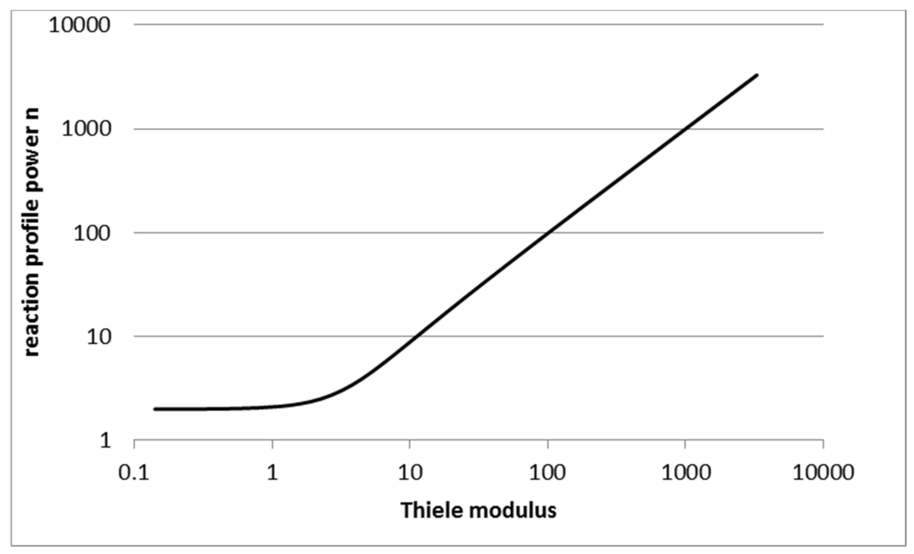
2.2. Choosing the Reaction Rate Profile

The reaction profile was assumed to be of a polynomial form with two terms. One is a constant, and the other is raised to a power depending on the relative reaction rate. It is expected that high values for this parameter will be encountered at high Thiele modulus values, and smaller values at low Thiele modulus values.

As the power n depends on the steepness of the reaction rate profile near the catalyst surface, its value can be obtained by setting reaction rate profile gradient at the surface equal to the linearized reaction rate multiplied by the composition profile gradient at the surface. The composition profile gradient is obtained with the present solution to the RDC equation (Equation (13)). This can be expressed as:

$$\frac{\mathrm{d}\mathrm{R}}{\mathrm{d}\mathrm{r}}=\frac{\mathrm{d}\mathrm{R}}{\mathrm{d}\mathrm{x}}\frac{\mathrm{d}\mathrm{x}}{\mathrm{d}\mathrm{r}}$$

(26)

After inserting all the terms at the catalyst surface conditions:

$$\mathrm{n}{\mathrm{b}}_{\mathrm{i}}{\mathrm{L}}^{\mathrm{n}-1}=\frac{\mathrm{d}{\mathrm{R}}_{\mathrm{L}\mathrm{i}}}{\mathrm{d}\mathrm{x}}\left(2{\mathrm{p}}_{1\mathrm{i}}\mathrm{L}+\left(\mathrm{n}+2\right){\mathrm{p}}_{2\mathrm{i}}{\mathrm{L}}^{\mathrm{n}+1}\right)$$

(27)

For the selection of appropriate reaction rate profile, convective part in p₁ (k in Equation (14)) was neglected to allow for explicit solution, although it was not neglected in the underlying RDC model. When the values for p₁ and p₂ were inserted, the non-linear terms (Lⁿ) cancel out favorably, leaving us a quadratic polynomial for n to be solved. The solution is:

$${\mathrm{n}}_{\mathrm{i}}=\frac{{\mathsf{\varphi }}_{\mathrm{i}}-\left(\mathrm{m}+1\right)+\sqrt{{\left(\mathrm{m}+1-{\mathsf{\varphi }}_{\mathrm{i}}\right)}^2+4\left({\mathrm{\Phi }}_{\mathrm{i}}^2+\left(\mathrm{m}+1\right){\mathsf{\varphi }}_{\mathrm{i}}\right)}}{2}$$

(28)

where the larger root was chosen for a physically meaningful solution. Maximum of the predicted n_i values for each component is selected, with a minimum set to n = 2.

In the previous equation, the following terms were defined:

$${\mathsf{\varphi }}_{\mathrm{i}}={\left(\left[\mathrm{B}\right]\frac{\mathrm{d}{\mathrm{R}}_{\mathrm{L}}}{\mathrm{d}\mathrm{x}}\right)}_{\mathrm{i}}\frac{{\mathrm{R}}_{0,\mathrm{i}}}{\left({\mathrm{R}}_{\mathrm{s},\mathrm{i}}+{\mathrm{R}}_{0,\mathrm{i}}\right)\left(\mathrm{m}+1\right)}$$

(29)

and:

$${\mathrm{\Phi }}_{\mathrm{i}}^2={\left(\left[\mathrm{B}\right]\frac{\mathrm{d}{\mathrm{R}}_{\mathrm{L}}}{\mathrm{d}\mathrm{x}}\right)}_{\mathrm{i}}{\mathrm{L}}^2$$

(30)

The latter is a square of the Thiele modulus for multicomponent systems in case of a first order reaction. Here, it was defined for each component separately. In this formulation, the reaction stoichiometry will be included in the modulus: it is based on the true formation rate of a component of interest, not the extent of reaction rate. With this approach, scaling of the stoichiometric ratios does not affect numerical values of the modulus. Diffusional interactions were also accounted for with non-diagonal elements of [B] [25]. For other than first order reactions, the present definition deviated from the original definition of the Thiele modulus by a constant factor, appearing due to differentiation of nonlinear reaction rates. However, in all cases, the present definition is directly proportional to the classical definition of Thiele modulus, and thus expresses the same physical ratio.

It can be seen from Equations (25)–(27) that when reaction rates were very high near the catalyst surface as compared to the center (high Thiele modulus values), the reaction rate profile exponent n became equal to the Thiele modulus. This can also be expressed so that at the diffusionally limited regime, the reaction rate is proportional to the distance from the catalyst center raised to a power equal to the Thiele modulus.

2.3. Finite Volume Solution

In order to validate the present approximation in general non-linear cases where analytical solution is not available, a reference solution with finite volume method was used. The finite volume method was formulated by dividing the catalyst particle into a number of control volumes following the catalyst particle symmetry as “shells”. The balance equations are constructed as follows: diffusion fluxes for nc-1 components at the control volume boundaries were calculated with central differences (compositions known at the center points of the control volumes, but fluxes needed at the boundaries) as:

$${\left(\mathrm{J}\right)}_{\mathrm{j}+1/2}={\mathrm{c}}_{\mathrm{t}}[\mathrm{D}]\frac{{\left(\mathrm{x}\right)}_{\mathrm{j}+1}-{\left(\mathrm{x}\right)}_{\mathrm{j}}}{{\mathrm{r}}_{\mathrm{j}+1}-{\mathrm{r}}_{\mathrm{j}}}$$

(31)

$${\left(\mathrm{J}\right)}_{\mathrm{j}+1/2,\mathrm{n}\mathrm{c}}=-{\displaystyle \sum _{\mathrm{i}=1}^{\mathrm{n}\mathrm{c}-1}{\left(\mathrm{J}\right)}_{\mathrm{j}+1/2,\mathrm{i}}}$$

(32)

$${\left(\mathrm{N}\right)}_{\mathrm{j}+1/2}={\left(\mathrm{J}\right)}_{\mathrm{j}+1/2}+{\mathrm{N}}_{\mathrm{t},\mathrm{j}+1/2}\frac{{\left(\mathrm{x}\right)}_{\mathrm{j}+1}+{\left(\mathrm{x}\right)}_{\mathrm{j}}}{2}$$

(33)

where at the center of the particle, fluxes are set to zero due to symmetry. Here, subscript j refers to the control volume number and i to component number.

Steady state material balances are then obtained from:

$${\mathrm{A}}_{\mathrm{j}-1/2}{\left(\mathrm{N}\right)}_{\mathrm{j}-1/2}-{\mathrm{A}}_{\mathrm{j}+1/2}{\left(\mathrm{N}\right)}_{\mathrm{j}+1/2}+{\left(\mathrm{R}\right)}_{\mathrm{j}}{\mathrm{V}}_{\mathrm{j}}=\left(0\right)$$

(34)

Additionally, mole fraction summation equations for each control volume are needed:

$${\displaystyle \sum _{\mathrm{i}=1}^{\mathrm{n}\mathrm{c}}{\mathrm{x}}_{\mathrm{j},\mathrm{i}}}=1$$

(35)

This set of equations (nc material balances and one summation equation) was solved for each control volume. The variables to be solved were the mole fractions of each component in each control volume, and total flux at each control volume boundary.

The effectiveness factors for finite volume method were obtained by first discretizing the particle radial coordinate with 100 and 200 equal size control volumes, and solving for mole fractions and total flux in each control volume. Effectiveness factor for each case was calculated by summing up each control volume reaction rates, and using Richardson extrapolation to these two discretized solutions for estimating the final effectiveness factor by assuming second order convergence. This was found to result in accurate enough effectiveness factors for our purposes when the Thiele modulus was not extremely high. With higher Thiele modulus values, non-uniform grid should be used so that smaller control volumes would be positioned near the catalyst surface where the reaction rates are the highest.

3. Results and Discussion

The predictive capability of the proposed approximate method was assessed with several numerical comparisons, each with different characteristic behavior. The first test was carried out with a first order reaction in three standard geometries for which analytical solutions are available: slab, cylinder, and sphere. The second test assumed elementary second order kinetics with a single reactant, again in the three standard geometries. This case was evaluated first by assuming that there was only pure reactant outside the catalyst, and then with reactant and 50% inert. The third test case was with elementary reaction for two reactants and non-stoichiometric surface compositions, which led to the depletion of one of the components and gradual change from second to pseudo-first order reaction as the reactants diffuse towards the catalyst particle center. The final test case was a realistic hydrogenation reaction, where the catalyst size effect was tested. For the test Cases (1) to (3), equal diffusivities of 10⁻⁹ m²/s were used with a total concentration of 50,000 mol/m³ and particle size of L = 0.001 m. Reaction rate coefficient was varied in order to vary the Thiele modulus values. Precise values of these physical parameters were not highly important in order to draw relevant conclusions, as they will always be lumped together in the model. For the final test case, realistic physical properties for the practical system were used, along with the Maxwell-Stefan diffusion model.

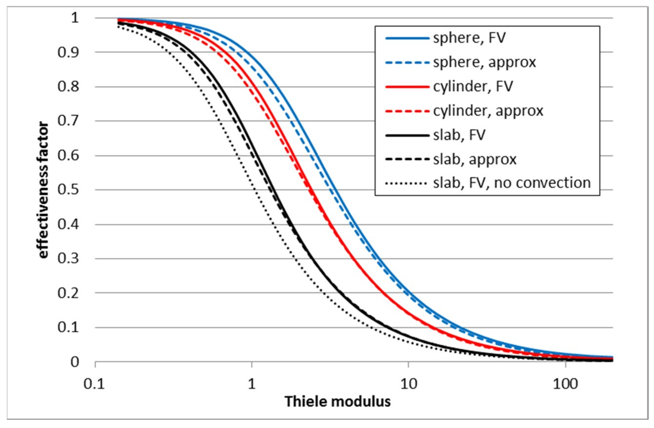
3.1. First Order Elementary Reaction A → B

The present approximate solution was first compared to the analytical solutions for a first order irreversible reaction. The reaction rate expression is:

$$\mathrm{R}={\mathrm{k}}_{\mathrm{r}}{\mathrm{x}}_{\mathrm{A}}$$

(36)

The test was carried out in various geometries: slab, cylinder, and spherical, as functions of a wide range of Thiele modulus values. The analytical solutions are:

$$\mathsf{\eta }=\frac{\tanh \left(\mathrm{\Phi }\right)}{\mathrm{\Phi }}\hspace{1em}\hspace{1em}\hspace{1em}\text{for slab}$$

(37)

$$\mathsf{\eta }=\frac{2{\mathrm{I}}_1\left(\mathrm{\Phi }\right)}{\mathrm{\Phi }{\mathrm{I}}_0\left(\mathrm{\Phi }\right)}\hspace{1em}\hspace{1em}\hspace{1em}\text{for cylinder}$$

(38)

$$\mathsf{\eta }=\frac{3\left(\mathrm{\Phi }\coth \left(\mathrm{\Phi }\right)-1\right)}{{\mathrm{\Phi }}^2}\hspace{1em}\hspace{1em}\hspace{1em}\text{for sphere}$$

(39)

In this test case, diffusional interactions are neglected: matrix [B] is diagonal, and it was further assumed that all the diffusion coefficients for each component were the same. Thus, the Thiele modulus in this case is:

$$\mathrm{\Phi }={\mathrm{k}}_{\mathrm{r}}\mathrm{B}{\mathrm{L}}^2$$

(40)

In Figure 1, the relative errors are shown for the three standard geometries.

It can be seen that the approximate solution approached the analytical solution asymptotically both for relatively low and very high Thiele modulus values. For the intermediate regime, the maximum relative error was around 3% and the maximum absolute error around 0.01 for predicted effectiveness factors. For cylindrical geometries, analytical solution was not possible above Thiele modulus values above 700 due to problems in the Matlab function “besseli” (the present approximate solution was nevertheless found rapidly); however, already smaller Thiele modulus values proved that the asymptotic behavior observed in Figure 1 holds also for cylinders.

Interestingly, as an example, the finite volume solution required at least 320 control volumes to achieve comparable accuracy with the suggested approximate solution with Thiele modulus of 100 for a spherical geometry. It took orders of magnitude more computational time to solve composition profiles even for a single catalyst particle compared to the approximate solution. It is highly probable that in practice, a much lower number of control volumes would be used to discretize the catalyst radius dimension than required for reasonable accuracy. This would lead to erroneous solution, although the control volume or other similar discretized solutions are expected to be “rigorous”.

In Figure 2, the profile power n is shown for spherical geometry. Powers for all geometries are very close to each other.

The asymptotic behavior of reaction profile power discussed earlier can be again seen from Figure 2. At high Thiele moduli, the reaction rate profile parameter n approaches Thiele modulus values.

Effect of particle geometry was also studied for this case. Intermediate Thiele modulus value (10 in this case), for which the relative error in the approximate method is the largest, was selected as a test case in order to emphasize potential discrepancies. The shape parameter was varied between −1/5 to 5, as suggested by [27]. As there is no analytical solution for the full range of shape factors, the finite volume solution was used as the reference. The results are shown in Figure 3.

It can be seen that the present approximation predicts effectiveness factors very accurately over a very wide range of particle shape factors.

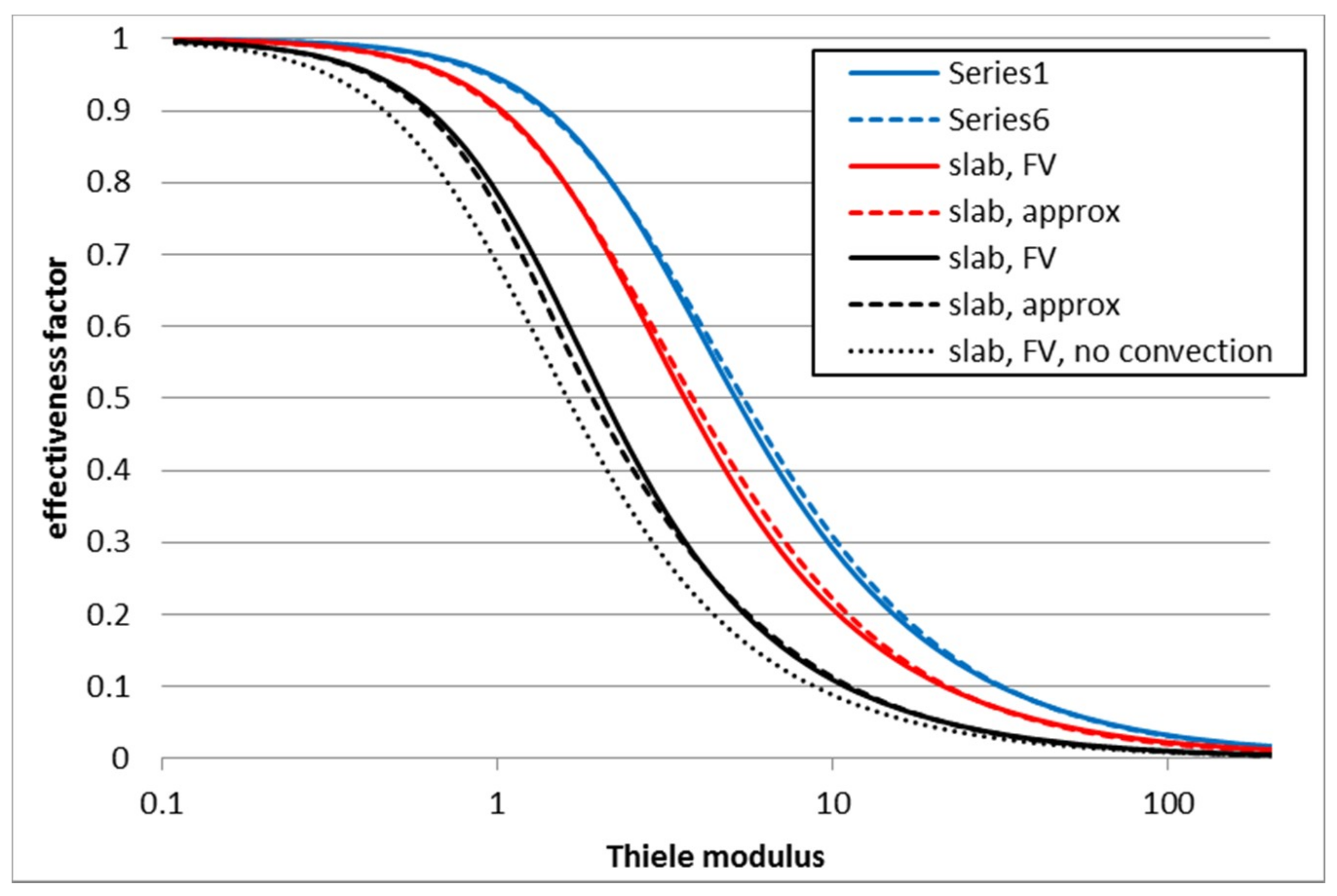
3.2. Second Order Reaction 2A → B

The second case was a simple second order elementary reaction with the following reaction rate:

$$\mathrm{R}={\mathrm{k}}_{\mathrm{r}}{\mathrm{x}}_{\mathrm{A}}^2$$

(41)

Although this case may seem to be close to the first test case, the reaction was non-equimolar inducing total convective flux towards the catalyst center. In this case, total flux increased effectiveness factor as net convection towards catalyst center carries reactants further along with diffusion. In Figure 4, the effectiveness factors predicted by the finite volume method and the corresponding effectiveness factors predicted by the present approximate solution are shown as functions of Thiele modulus. Here, the classical definition of Thiele modulus [4] was used for x-axis instead of definition by Equation (27). Maximum error in the effectiveness factors were 0.028 for slab and cylinder and 0.038 for sphere. For comparison, the effectiveness factors calculated with the finite volume method but neglecting convective mass transfer are shown. This was done so that the total fluxes in the finite volume solution were set to zero and the last material balance was replaced by the summation equation. Without this replacement, the finite volume model did not converge. However, it must be noted that the RDC equation was not satisfied for the last component after this modification. The maximum error in the effectiveness factor when neglecting total flux was around 0.11, and it was the same for all geometries. Results for the slab geometry are shown to keep the graph simple. It can be seen that the present approximation follows the rigorous solution closely, with the error being much smaller compared to the error caused by a regrettably common assumption of negligible convective flux.

Further tests were carried out with the same reaction scheme as before; however, specifying surface compositions as 50 mol % reactant A and 50 mol % of inert. This deviates from the previous case since inert is accumulating in the catalyst interior due to convective flux; its convective flux towards the center was balanced by a diffusion flux out. This behavior (solution of composition profiles with the FV model) with Thiele modulus of 10 and m = 2 (spherical geometry) are shown in Figure 5.

The maximum errors in effectiveness factors calculated with the proposed approximate solution with a wide range of Thiele modulus values were 0.027, 0.027, and 0.034 for slab, cylinder, and sphere, respectively.

3.3. Second Order Reaction A + B → C

In this case, the reaction rate expression is:

$$\mathrm{R}={\mathrm{k}}_{\mathrm{r}}{\mathrm{x}}_{\mathrm{A}}{\mathrm{x}}_{\mathrm{B}}$$

(42)

If concentrations of A and B outside the particle are the same, the results are equivalent to the case 2A → B. However, if the mole fractions of A and B are not equal outside the catalyst particle, the reaction remains practically of second order near the surface, but in cases of high reaction rates becomes a pseudo-first order deeper in the catalyst where the limiting component has been almost fully consumed. In order to study this behavior, the surface mole fractions were set to 0.6 for A and 0.4 for B. Results are shown in Figure 6. Maximum errors in the effectiveness factors in this case were 0.035, 0.024, and 0.019 for the slab, cylinder, and sphere, respectively.

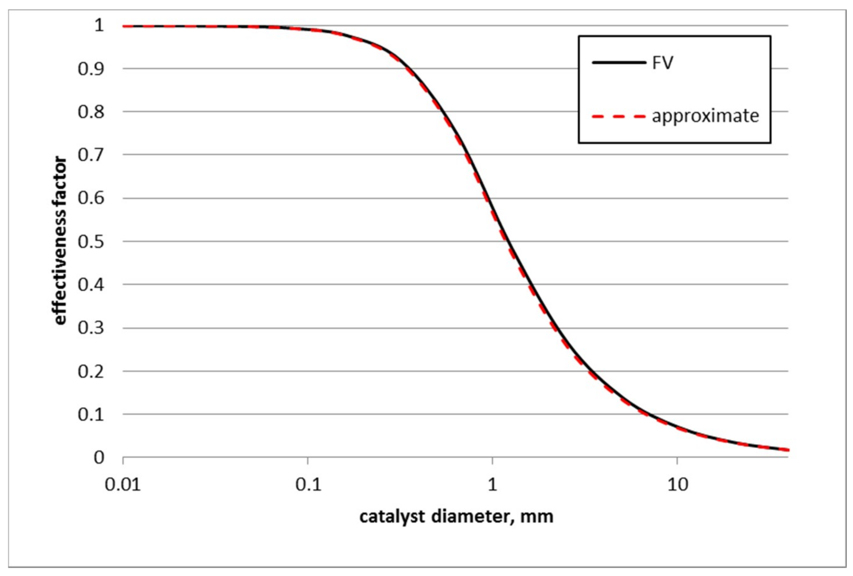
3.4. Effect of Catalyst Size on Toluene Hydrogenation

The final test case is hydrogenation of toluene inside porous catalyst particles. This case is just an illustration when the present model was applied to a real case where kinetic expression is known; any other industrially relevant case could have been selected as well.

The kinetics of this reaction were given by [28] (Model I, heterogeneous reactor model, dissociative adsorption of hydrogen, temperature equal to the reference temperature of 100 °C), and they follow Langmuir-Hinshelwood kinetics. The stoichiometry of this reaction is:

C₇H₈ + 3H₂ → C₇H₁₄

(43)

The reaction rate per total solid catalyst mass is:

$${\mathrm{R}}_{\mathrm{m}}=\frac{{\mathrm{k}}_1{\mathrm{K}}_{\mathrm{A}}{\mathrm{K}}_{\mathrm{H}}{\mathrm{c}}_{\mathrm{A}}{\mathrm{c}}_{\mathrm{H}}}{{\left(3{\mathrm{K}}_{\mathrm{A}}{\mathrm{c}}_{\mathrm{A}}+{\left({\mathrm{K}}_{\mathrm{H}}{\mathrm{c}}_{\mathrm{H}}\right)}^{0.5}+1\right)}^3}$$

(44)

where k₁ = 2.1 mol/(s kg); K_A = 2.5 × 10⁻⁴ m³/mol; K_H = 3.69 × 10⁻² m³/mol.

Here, A refers to the aromatic compound (toluene) and H to hydrogen. The dimension of R_m was mol/(s kg catalyst). The density of catalyst was 1300 kg/m³ and porosity 0.5, so that total reaction rate per volume of fluid inside catalyst was:

$$\mathrm{R}={\mathrm{R}}_{\mathrm{m}}\frac{{\mathsf{\rho }}_{\mathrm{C}}}{1-\mathsf{\epsilon }}$$

(45)

Cylindrical catalyst particles were assumed in this study. The cylinders were assumed long compared to the diameter, so that we have m = 1 for the geometry parameter. The surface mole fractions were assumed to be 0.1 for hydrogen, 0.7 for toluene, and 0.2 for methylcyclohexane.

Binary diffusion coefficients were estimated with Wilke-Chang method [29]. Those binary diffusion coefficients where hydrogen should have been assumed as a solvent were neglected, and the binary diffusion coefficient matrix was assumed symmetrical. The binary diffusion coefficients were:

D_HA = D_AH = 1.32504 × 10⁻⁸ m²/s

(46)

D_HS = D_SH = 1.21466 × 10⁻⁸ m²/s

(47)

D_AS = D_SA = 5.18374 × 10⁻⁸ m²/s

(48)

where subscript S refers to the saturated product (C₇H₁₄). Maxwell-Stefan diffusion coefficient matrix [D] was calculated as in [25]. For the discretized control volume model, mole fractions from each control volume were used separately; however, for the simplified method based on reaction rate profiles, mole fractions at the particle surface were used. In this way, we avoided updating the diffusion coefficient matrix during the iteration. This is consistent with suggestions for the Maxwell-Stefan approach for the film model [30]. The average total concentration for this system was assumed to be constant, 9000 mol/m³.

Predicted effectiveness factors with the proposed approximation as well as finite volume method are shown in Figure 7.

It can be seen that the present model approximates effectiveness factors extremely well. The maximum absolute error in the predicted effectiveness factor was 0.013 and relative error 4% with a very wide range of catalyst diameters studied. The real hydrogenation process was possibly partially limited by diffusion in catalyst within industrially relevant catalyst size ranges, as also noted by [28]. Hence, it is important to have a reasonable estimate for the effectiveness factors in practical reactor simulations. The approximate method proposed in this work gives opportunity to do this in an efficient manner.

4. Conclusions

An approximate method for solving reaction-diffusion-convection problems within catalyst particles was developed in this work. The underlying idea behind the present approximation was that the reaction rate profile as a function of location was assumed instead of the traditionally assumed composition profiles. This allowed a simple analytical solution of the reaction-diffusion-convection equation with the approximate profiles. The reaction rate profile was found by setting the reaction rate gradients at the catalyst surface equal to the linearized reaction kinetics. Intrinsic chemical kinetics were also used for the reaction rate profile coefficients.

The present method was compared with available analytical solutions as well as with rigorous finite volume solution, first in a number of ideal reaction schemes and then with an industrially important catalytic reaction for toluene hydrogenation. It was shown that the present approximation was capable of describing a variety of multicomponent reactions in various catalyst geometries with excellent accuracy. Furthermore, it was shown that significant errors could result from neglecting the convective flux in the model for non-equimolar reaction stoichiometries. Thus, improper but common model formulation was expected to lead to more erroneous results than the approximate solution proposed here.

References

1. Aris, R. The Mathematical Theory of Diffusion and Reaction in Permeable Catalysts. Vol I. The Theory of the Steady State; Clarendon Press: Oxford, UK, 1975. [Google Scholar]
2. Bird, R.B.; Stewart, W.E.; Lightfoot, E.N. Transport Phenomena; Wiley: New York, NY, USA, 1960. [Google Scholar]
3. Fogler, S. Elements of Chemical Reaction Engineering, 4th ed.; Prentice Hall: Englewood Cliffs, NJ, USA, 2006. [Google Scholar]
4. Levenspiel, O. Chemical Reaction Engineering, 2nd ed.; Wiley: New York, NY, USA, 1972. [Google Scholar]
5. Finlayson, B.A. Nonlinear Analysis in Chemical Engineering; McGraw-Hill: New York, NY, USA, 1980. [Google Scholar]
6. Rice, R.G.; Do, D.D. Applied Mathematics and Modeling for Chemical Engineers; Wiley: New York, NY, USA, 1995. [Google Scholar]
7. Villadsen, J.; Michelsen, M.L. Solution of Differential Equation Models by Polynomial Approximation; Prentice-Hall: Englewood Cliffs, NJ, USA, 1978. [Google Scholar]
8. Russo, V.; Kilpiö, T.; Di Serio, M.; Tesser, R.; Santacesaria, E.; Murzin, D.Y.; Salmi, T. Dynamic non-isothermal trickle bed reactor with both internal diffusion and heat conduction: Sugar hydrogenation as a case study. Chem. Eng. Res. Des. 2015, 102, 171–185. [Google Scholar] [CrossRef]
9. Thiele, E.W. Relation between Catalytic Activity and Size of Particle. Ind. Eng. Chem. Res. 1939, 31, 916–920. [Google Scholar] [CrossRef]
10. Gottifredi, J.C.; Gonzo, E.E.; Quiroga, O.D. Isothermal Effectiveness Factor—I Analytical expression for single reaction with arbitrary kinetics. Slab geometry. Chem. Eng. Sci. 1981, 36, 705–711. [Google Scholar]
11. Gottifredi, J.C.; Gonzo, E.E.; Quiroga, O.D. Isothermal Effectiveness Factor—II Analytical expression for single reaction with arbitrary kinetics, geometry and activity distribution. Chem. Eng. Sci. 1981, 36, 713–719. [Google Scholar] [CrossRef]
12. Haynes, H.W. An explicit approximation for the effectiveness factor in porous heterogeneous catalysts. Chem. Eng. Sci. 1986, 41, 412–415. [Google Scholar] [CrossRef]
13. Kim, D.H.; Lee, J. A simple formula for estimation of the effectiveness factor in porous catalysts. AIChE J. 2006, 52, 3631–3635. [Google Scholar] [CrossRef]
14. Kubota, H.; Yamanaka, Y. Remarks on approximate estimation of catalyst effectiveness factor. J. Chem. Eng. Jpn. 1969, 2, 238–240. [Google Scholar] [CrossRef]
15. Lee, J.; Kim, D.H. An approximation method for the effectiveness factor in porous catalysts. Chem. Eng. Sci. 2006, 61, 5127–5136. [Google Scholar] [CrossRef]
16. Marroquin de la Rosa, J.O.; Garcia, T.V.; Ochoa Tapia, J.A. A linear approximation method to evaluate isothermal effectiveness factors. Chem. Eng. Commun. 1999, 174, 53–60. [Google Scholar] [CrossRef]
17. Wedel, S.; Luss, D. A rational approximation of the effectiveness factor. Chem. Eng. Commun. 1980, 7, 245–254. [Google Scholar] [CrossRef]
18. Yin, Q.; Li, S. Rational Approximation of the Overall Effectiveness Factor for the Gas-Liquid-Solid Phase Catalytic Reaction. Ind. Eng. Chem. Res. 1995, 34, 3771–3776. [Google Scholar] [CrossRef]
19. Aris, R. On the shape factors for irregular particles—I The steady state problem. Diffusion and reaction. Chem. Eng. Sci. 1957, 6, 262–268. [Google Scholar] [CrossRef]
20. Burghardt, A.; Kubaczka, A. Generalization of the effectiveness factor for any shape of a catalyst pellet. Chem. Eng. Process. 1996, 35, 65–74. [Google Scholar] [CrossRef]
21. Mariani, N.J.; Mocciaro, C.; Keegan, S.D.; Martinez, O.M.; Barreto, G.F. Evaluating the effectiveness factor from a 1D approximation fitted at high Thiele modulus: Spanning commercial pellet shapes with linear kinetics. Chem. Eng. Sci. 2009, 64, 2762–2766. [Google Scholar] [CrossRef]
22. Liu, Z.; Suntio, V.; Kuitunen, S.; Roininen, J.; Alopaeus, V. Modeling of mass transfer and reactions in anisotropic biomass particles with reduced computational load. Ind. Eng. Chem. Res. 2014, 53, 4096–4103. [Google Scholar] [CrossRef]
23. Salmi, T. Computer Aided Chemical Reaction Engineering. Lecture Notes; Åbo Akademi: Turku, Finland, 1996. [Google Scholar]
24. Gorshkova, E.; Manninen, M.; Alopaeus, V.; Laavi, H.; Koskinen, J. Three-Phase CFD-Model for Trickle Bed Reactors. Int. J. Nonlinear Sci. Numer. Simul. 2012, 13, 397–404. [Google Scholar] [CrossRef]
25. Taylor, R.; Krishna, R. Multicomponent Mass Transfer; Wiley: New York, NY, USA, 1993. [Google Scholar]
26. Jackson, R. On the limit of bulk diffusion control and high permeability in porous catalyst pellets. Chem. Eng. Sci. 1974, 29, 1413–1419. [Google Scholar] [CrossRef]
27. Keegan, S.D.; Mariani, N.J.; Bressa, S.P.; Mazza, G.D.; Barreto, G.F. Approximation of the effectiveness factor in catalyst pellets. Chem. Eng. J. 2003, 94, 107–112. [Google Scholar] [CrossRef]
28. Toppinen, S.; Rantakylä, T.-K.; Salmi, T.; Aittamaa, J. Kinetics of the Liquid-Phase Hydrogenation of Benzene and Some Monosubstituted Alkylbenzenes over a Nickel Catalyst. Ind. Eng. Chem. Res. 1996, 35, 1824–1833. [Google Scholar] [CrossRef]
29. Reid, R.C.; Prausnitz, J.M.; Poling, B.E. Properties of Gases & Liquids, 4th ed.; McGraw-Hill: New York, NY, USA, 1987. [Google Scholar]
30. Alopaeus, V.; Aittamaa, J. Appropriate simplifications in calculation of mass transfer in a multicomponent rate-based distillation tray model. Ind. Eng. Chem. Res. 2000, 39, 4336–4345. [Google Scholar] [CrossRef]
Figure 1. Relative errors in the effectiveness factors for the three standard geometries as functions of Thiele modulus.
Catalysts 09 00255 g001
Figure 2. Reaction rate profile power as a function of Thiele modulus for spherical geometry.
Catalysts 09 00255 g002
Figure 3. Effectiveness factor as a function of particle shape factor with Thiele modulus value of 10 for the finite volume (FV) and the present approximate solutions.
Catalysts 09 00255 g003
Figure 4. Effectiveness factors for second order elementary reactions in three geometries with finite volume and approximate method. Effectiveness factor for slab when convective flux is neglected is shown for reference.
Catalysts 09 00255 g004
Figure 5. Composition profiles for second order elementary reaction 2A → B with inert compound.
Catalysts 09 00255 g005
Figure 6. Effectiveness factors for second order elementary reaction A + B → C with non-stoichiometric feed in three geometries with finite volume and approximate method. Effectiveness factors for slab when convective flux is neglected is shown for reference.
Catalysts 09 00255 g006
Figure 7. Effectiveness factors for toluene hydrogenation case as functions of particle size.
Catalysts 09 00255 g007