Mechanism-Guided Selective Hydrogenation of CO₂ to Light Olefins: DFT-Informed Microkinetics and Surface Electronic Regulation Under Green Hydrogen Scenarios

Abstract

Achieving high selectivity in the hydrogenation of CO₂ to light olefins remains challenging because of the complex reaction network and the difficulty of regulating key intermediates. Motivated by green-hydrogen-enabled power-to-chemicals pathways, we combine density functional theory (DFT) with first-principles microkinetic simulation (FPMS) to construct a quantitatively predictive reaction-energy landscape and elucidate structure–selectivity relationships. A comprehensive reaction network is established through energy-surface fitting, and steady-state rate constants are solved to capture the microkinetic competition between elementary steps. By introducing electronic density-of-states (DOS) modulation as a design variable, we directly correlate surface structural parameters with rate-controlling steps, thereby enabling targeted regulation of C–C coupling and hydrogen transfer processes. The calculated barrier for CO₂ adsorption to COOH* is 1.35 eV, while the transition state barrier for C–C coupling is 1.50 eV, corresponding to a reaction rate of 9.7 × 10³ s⁻¹; the olefin desorption rate reaches 1.7 × 10⁷ s⁻¹. Crucially, shifting the d-band center from −2.35 eV to −1.60 eV increases the C₂–C₄ olefin selectivity from 42.6% to 68.3%, establishing an actionable electronic structure lever for catalyst optimization. These results reveal the intrinsic mechanism by which surface electronic and geometric regulation governs intermediate stabilization and rate control, providing a verifiable, mechanism-based design principle for efficient CO₂-to-olefin catalysts aligned with green hydrogen deployment.

1. Introduction

The hydrogenation of carbon dioxide (CO₂) to light olefins is a pivotal route for efficient carbon resource utilization and the establishment of a circular carbon economy, with profound implications for mitigating the greenhouse effect and advancing green chemistry [1,2,3]. As fundamental platform chemicals, light olefins possess high added value and robust market demand, which has intensified research interest in CO₂ hydrogenation as a sustainable production pathway [4,5,6]. Catalytically transforming this thermodynamically stable molecule into target hydrocarbons not only reduces carbon emissions but also enables carbon reutilization [7,8]. Nevertheless, the high intrinsic stability of CO₂ and the complexity of its multi-step reaction network render the attainment of highly selective light olefin formation under energy-efficient conditions a central scientific challenge in heterogeneous catalysis [9,10].

Key obstacles arise from the low activation efficiency of CO₂ and the severe competition between parallel pathways during hydrogenation [11,12]. CO₂ can evolve through multiple routes—most prominently via CO* or formate-type intermediates—but these species compete during surface adsorption, conversion, and desorption, broadening product distributions and diminishing the selectivity [13,14]. In addition, the carbon–carbon coupling step typically presents a substantial kinetic barrier that limits light olefin formation. Heterogeneities in active sites and the lack of precise control over the surface electronic structure further skew the balance between hydrogenation and dehydrogenation events, depressing the yield of desired products [15,16]. Consequently, precise control over the intermediate stability and the distribution of reaction energy barriers within a complex, multipath environment has become the principal bottleneck to improving selectivity toward light olefins [17,18].

A variety of strategies have been explored to confront these issues [19,20]. Structure-guided catalyst design—through alloying, support engineering, or defect/strain modulation—can enhance CO₂ adsorption and activation; however, predictive, quantitative links between structural descriptors and the distribution of energy barriers often remain empirical and incomplete [21,22]. Multifunctional catalytic systems introduce synergistic activation and coupling sites, yet their intricate interfacial architectures are difficult to stabilize under realistic reaction conditions [23,24]. Although reaction kinetics modeling and potential energy surface calculations illuminate key mechanistic aspects, they frequently overlook how electronic structure perturbations reshape intermediate adsorption energetics, leading to gaps between theory and experiment [25,26]. As a result, a rigorous, quantitative correlation between structural regulation and pathway-specific kinetics is still lacking—an omission that fundamentally constrains progress in light olefin selectivity.

To address the incomplete coupling between structural regulation and reaction pathways, this work develops a first-principles microkinetic simulation (FPMS) framework built on a high-fidelity reaction-pathway energy surface. Based on density functional theory (DFT), we calculate the adsorption energies, transition-state barriers, and potential-energy profiles of key intermediates involved in CO₂ hydrogenation at the atomic scale. These data are then incorporated into a microkinetic model to derive steady-state rate constants and establish a quantitatively predictive description of the reaction network. Importantly, by integrating an electronic density-of-states (DOS) regulation strategy, parameterized through variations in surface configuration and the d-band center, we enable directional control over the rate-determining C–C coupling and hydrogen transfer steps. In this way, the framework establishes a quantitative link between electronic structure regulation and kinetic behavior, clarifies how specific structural parameters govern product distributions, and provides a mechanistically grounded basis for the rational design of catalysts for highly selective CO₂-to-light-olefin conversion.

2. Results and Discussion

2.1. Reaction Path and Energy Distribution Analysis

In the study of reaction pathways and energy distribution, a systematic comparative analysis of experimental measurements and computational analyses was conducted to verify the reliability of microscopic kinetic simulations and reveal the intrinsic connection between energy evolution and structural effects during the hydrogenation of CO₂ to light olefins. By testing the activation behavior of different metal–oxide composite catalysts in a fixed-bed reactor, data on the adsorption states and reaction energy barriers of key intermediates were obtained. Combined with the rate constants derived from first-principles calculations, the reaction pathway energy surface was reconstructed. Furthermore, a valence band center manipulation strategy was employed to investigate the effects of electronic structure changes on adsorption strength and reaction rate. A multidimensional correlation between the reaction pathway energy, rate constants, and adsorption energy was established from both experimental and simulation perspectives, yielding the results shown in Figure 1.

Reaction energy distributions reveal that the energy barrier for CO₂ adsorption to form COOH* is 1.35 eV, while the transition state barrier for C–C coupling reaches 1.50 eV, reflecting the energy-limited nature of the surface carbon species polymerization process. This barrier difference stems from the uneven distribution of electron density within the metal–carbon coordination in the activated transition state, which leads to the enhanced localization of bond stretching vibration modes and, in turn, raises the reaction barrier. Rate constants reveal that the reaction rate for the C–C coupling step is only 9.7 × 10³ s⁻¹, while the rate for the C₂H₄ desorption process reaches 1.7 × 10⁷ s⁻¹. This order-of-magnitude difference is closely related to the degree of interface electronic state localization. As the d-band center shifts from −2.1 eV to −0.9 eV, the CO adsorption energy decreases from −1.25 eV to −1.70 eV, reflecting that increased electron filling leads to enhanced antibonding orbital overlap, increasing the adsorption bond energy and limiting the desorption process. The energy surface elevation and rate reduction together characterize the trend of reaction barrier migration under the regulation of the surface electronic structure, indicating that the center position of the catalyst valence band has a decisive influence on the carbon–carbon coupling kinetics.

2.2. Correlation Between Intermediate Adsorption Behavior and Electronic Structure

In the following discussion, species marked with * refer to adsorbed intermediates on the catalyst surface. In electronic structure manipulation experiments, to investigate the influence of the distribution of electronic states on the catalyst surface on the adsorption behavior of key intermediates and the reaction steps, metal–oxide composite catalyst samples with different d-band center positions were selected. Synchrotron ultraviolet photoelectron spectroscopy (UPS) was combined with first-principles calculations to obtain their valence band electron density distributions. The adsorption energies of key intermediates *CO₂, *CO, *CH₂, and *C₂H₄ at different electronic states were further calculated, thereby establishing a quantitative relationship between the adsorption strength and electronic structure. Simultaneously, by fitting the density of states (DOS) distributions and C–C coupling energy barriers of typical catalysts, the role of the upward shift of the valence band center on the reaction path selection was analyzed. These results, when combined, form a systematic understanding of the coupled effects of electronic structure and adsorption behavior, as shown in Figure 2.

As the d-band center shifts from −3.5 eV to −2.0 eV, the adsorption energy of *CO₂ decreases from −0.42 eV to −1.04 eV, and that of CO decreases from −0.68 eV to −1.20 eV, indicating enhanced coupling of the surface electron cloud density to the reacting molecular orbitals. This trend stems from increased d-orbital occupancy, which reduces antibonding orbital filling, thereby stabilizing the adsorbed intermediates. The density of states (DOS) distribution shows that as the valence band center approaches the Fermi level, the density of states in the energy range of −2 to 0 eV increases from 1.9 to 2.9, indicating enhanced surface-active electron donation and enhanced transition state stability for C–O and C–H bonding. The C–C coupling barrier decreases from 1.62 eV to 1.10 eV as the CO adsorption energy decreases, indicating that stronger surface adsorption promotes cooperative coupling between carbon species and reduces the energy barrier for carbon chain formation. This fine-tuning of the electronic structure alters the surface adsorption kinetics, making the light olefin formation pathway more energetically competitive.

2.3. Effect of Structural Parameters on the Formation of Light Olefins

To explore the effects of support and metal loading parameters on the performance of light olefin production, this study systematically varied the metal/support ratio, average metal particle size, d-band center position, and reaction temperature and metal loading coupling conditions under the same catalyst precursor and feed conditions. Gas chromatography and online mass spectrometry were used to simultaneously monitor the product distribution, and the catalyst surface structure was characterized by transmission electron microscopy and X-ray photoelectron spectroscopy. The experimental process included precursor impregnation, reduction treatment, catalytic reaction testing, and correlation analysis of the characterization data. The resulting multidimensional data were summarized to form a correlation map between structural parameters and reaction performance, as shown in Figure 3.

From the correspondence between the quantitative data and the characterization results, it can be seen that when the metal/support ratio is 0.2, the C2–C4 olefin selectivity is 42.3, and as the ratio increases to 1.0, the selectivity increases to 68.4. Within this range, the methane selectivity decreases from 28.1 to 16.7, indicating that higher metal loading increases the density of active sites available for skeleton reorganization and reduces the relative contribution of over-hydrogenation channels. When the average particle size corresponding to different crystal planes ranges from 9.8 nm to 13.7 nm, the carbon conversion rate fluctuates between 33.2 and 42.7, while the site geometry and low carbonization rate related to the particle size are significantly different. The coordination site ratio leads to olefin selectivity varying between 45.6 and 68.4. The higher olefin selectivity associated with smaller average particle size is attributed to the increased proportion of high-energy sites on the surface. When the d-band center shifts from −2.35 eV to −1.60 eV, the C2–C4 olefin selectivity increases from 42.6 to 68.3 and then decreases to 63.5. This suggests that the d-band position adjustment alters the adsorption strength and the energy barrier for dissociation/hydrogenation of the reaction intermediates, leading to an optimal electronic state for maximizing olefin yield. A coupled mapping of metal loading and temperature reveals that the olefin yield reaches 43.8 at 8 wt% metal loading and 380 °C. Excessive temperature and excessive loading increases the rate of side reactions and intensifies particle agglomeration, respectively, leading to a decrease in the yield. Mechanistically, this is the result of a competition between active site accessibility and selectivity. Taken together, these results suggest that structural parameters jointly determine olefin yield and selectivity by altering the geometry and electronic properties of the active sites, as well as the thermodynamic/kinetic balance.

2.4. Comparison of Dynamic Simulation Results with Experiments

In the carbon dioxide hydrogenation reaction system, to further reveal the influence of different generation pathways on product distribution and reaction rate, this study conducted a series of reaction kinetics experiments on a fixed-bed microreactor and analyzed the energy changes of each key intermediate in combination with density functional theory calculations. By controlling the reaction temperature and hydrogen partial pressure, experimental product selectivity data under various conditions were obtained and compared with the simulation results of the reaction kinetic model to verify the reliability of the model in capturing multi-step reaction rates and product evolution trends. Based on the calculation of reaction path rate constants and energy barrier distribution, the rate-control link in the key intermediate conversion process was evaluated, thus constructing a multi-layer verification system of experiment–simulation–theory. The results are shown in Figure 4.

The experimental selectivities of the reaction products generally agree well with the simulation results. The experimental selectivity for ethylene is 27.9%, while the simulated value is 28.6%, with a deviation of less than 1%, indicating that the model accurately describes the formation and conversion of C2 species. The experimental selectivities for propylene and butene are 24.8% and 13.9%, respectively, compared with the simulated values of 25.4% and 14.4%, respectively, with errors within the statistical range. This is closely related to the controlling role of the hydrogen adsorption–insertion equilibrium in the surface carbon chain extension step. The rate constants are distributed on the order of 10⁴. The CH₂→CH₂ coupling step reaches 9.1 × 10⁴ s⁻¹, indicating a low activation energy for this pathway. The initial CO₂ dissociation step is only 1.2 × 10⁴ s⁻¹, corresponding to an energy barrier of 1.10 eV, making it the rate-determining step in the entire reaction network. The energy profile reveals that the stabilization of the intermediate CH₂ reduces the energy barrier for subsequent carbon chain extension reactions to approximately 0.52 eV, promoting the formation of multi-carbon products. Therefore, the experimental and calculation results jointly indicate that the carbon–oxygen bond-breaking step dominates the reaction rate, while the surface hydrogen overflow and carbon chain growth processes mainly affect the relative distribution of alkenes and alkanes.

2.5. Analysis of Reaction Stability and Catalytic Mechanism

To investigate how the time-dependent structural and surface chemical evolution of the catalyst correlates with product distribution under fixed-bed flow reaction conditions, this experiment conducted long-term catalytic testing in continuous-feed mode and simultaneously implemented multimodal characterization: online gas chromatography was used to record the product conversion and selectivity over time, in situ XPS was used to monitor the metal valence changes over time, TEM and surface area measurements were combined to assess the morphology and surface area evolutions, and temperature-programmed desorption and in situ FTIR were used to identify surface carbon species. These time-resolved data were processed to construct the following graphs, which visualize the coupled relationship between catalyst performance and microscopic properties. The results are shown in Figure 5 below.

Analysis of the data in the figure shows that the CO₂ conversion rate reached a maximum of 42.4% at 40 h and maintained at 41.9% at 120 h. The selectivity of light olefins was 68.4% at 40 h and dropped to 67.8% at 120 h. The methane selectivity increased from 17.3% at 40 h to 18.0% at 120 h. At the same time, the metal phase to oxidation state ratio M⁰/Mⁿ⁺ decreased from the initial 1.00 to 0.95 at 120 h, while the surface graphitized carbon increased from 0.05 to 0.07, and the state density near the Fermi energy decreased from 3.2 to 3.0. These numerical changes are primarily attributed to the synergistic effects of two microscopic factors: First, slight oxidation of the metal surface reduces the electron-donating capacity, which slightly weakens the electronic coupling and activation of adsorbed species and leads to a small decrease in the density of states near the Fermi energy, thus slightly suppressing the overall activity. Second, the accumulation of graphitized components within the surface carbon species indicates the presence of trace amounts of irreversible carbon deposition. This deposition, as the ratio increases from 0.05 to 0.07, gradually reduces the number of available active sites and alters the local hydrogen coverage, leading to a slight increase in methane selectivity and a slight decrease in light olefin selectivity. Overall, the data indicate that the catalyst maintained near-steady-state high selectivity and activity over the 120 h run, with minor fluctuations in performance primarily attributable to slight oxidation of the metal surface and the accumulation of small amounts of graphitized carbon.

3. Materials and Methods

3.1. Catalyst Preparation and Structural Characterization

To validate the reliability of the simulation results and analyze the influence of structural factors on catalytic performance, a series of metal–oxide composite catalysts were prepared using an impregnation–reduction method. Differentiated surface structures were achieved by adjusting the metal type, loading, and support composition.

After drying, calcination, and reduction, the samples were characterized by X-ray diffraction (XRD, D8 Advance, Bruker, Karlsruhe, Germany) to determine their crystalline structure. Specific surface area and pore structure were measured by the Brunauer–Emmett–Teller (BET) method using an ASAP 2460 analyzer (Micromeritics, Norcross, GA, USA). Metal dispersion was determined by H₂ chemisorption using a Chemisorb 2720 instrument (Micromeritics, Norcross, GA, USA).

Data analysis and visualization were performed using OriginPro 2024 (OriginLab Corporation, Northampton, MA, USA). The structural parameter data for representative samples are presented in

Table 1. Statistical overview of experimental datasets.

Sample ID	Metal Type (wt%)	Specific Surface Area (BET, m2·g−1)	Average Crystallite Size (XRD, nm)	Metal Dispersion (H2 Chemisorption, %)
C-1	Ni 5.0	112	12.4	18.7
C-2	Ni 10.0	98	9.1	24.3
C-3	Fe 5.0	135	10.8	16.2
C-4	Ni–Fe (5:5, total metal 10.0)	127	8.6	28.9
C-5	Co 8.0	104	11.6	21.0
C-6	Ni 10.0 (support-modified SiO2—Al2O3)	148	7.9	33.5

.

This table lists the key structural parameters of catalysts with different metal systems and support configurations, demonstrating the influence of preparation conditions on specific surface area and crystallite size. The specific surface area and crystallite size were determined by XRD and BET methods, while metal dispersion was calculated by H₂ chemisorption. Comparison of these parameters provides fundamental data support for subsequent analysis of the correlation between reaction performance and structure.

This study selected the Ni–Fe bimetallic system as the core research object based on its tunable electronic structure and synergistic catalytic effect. Fe-based catalysts exhibit high selectivity for low-carbon olefins in CO₂ hydrogenation, while the introduction of Ni effectively promotes H₂ dissociation and regulates the hydrogenation rate of surface carbon species. Compared with single Fe/SiO₂ catalysts, the Ni–Fe bimetallic interface optimizes the adsorption energy of key intermediates through electronic effects, thereby more effectively regulating the competition between C–C coupling and the hydrogenation pathway. To verify this selection,

Table 2. Comparison of structural and performance parameters between Ni-Fe and reference Fe/SiO₂ catalysts.

Catalyst	Metal Dispersion (%)	Initial CO2 Conversion (%)	Initial C2–C4 Olefin Selectivity (%)
Ni–Fe/SiAl (C-4)	28.9	38.5	62.4
Fe/SiO2	19.6	35.2	58.1

compares the structure and initial performance of a representative Ni–Fe catalyst and a reference Fe/SiO₂ catalyst.

3.2. Reaction Apparatus and Conditions

To validate the reaction trends predicted by the microkinetic model and explore the reaction kinetics of CO₂ hydrogenation to light olefins under structurally controlled conditions, this study conducted a series of experiments in a fixed-bed flow reactor. By varying the H₂/CO₂ ratio, reaction temperature, pressure, and gas space velocity, we investigated the effects of reactant hydrogen supply intensity, energy input, and residence time on the carbon species conversion pathways. The experimental apparatus was equipped with an automated gas inlet and temperature and pressure control system, and products were monitored online by gas chromatography, enabling quantitative analysis under steady-state conditions.

Table 3. Fixed bed reaction conditions and gas ratio parameters.

Reaction No.	H2/CO2 Molar Ratio	Reaction Temperature (°C)	Reaction Pressure (bar)
R1	2.0	250	1.0
R2	3.0	280	1.0
R3	4.0	300	3.0
R4	3.0	320	5.0
R5	5.0	280	1.5
R6	3.0	260	2.0

lists the key operating parameters for each experimental condition for subsequent comparison of results and mechanistic correlation.

Under low-temperature and low-hydrogen-ratio conditions, the reaction is mainly limited by the CO₂ activation step. At 250 °C and a hydrogen-to-carbon ratio of 2.0 (R1), the relatively low hydrogen supply and insufficient reduction of surface oxidized metal active sites hinder the conversion of adsorbed CO₂. When the hydrogen-to-carbon ratio increases to 3.0 and the temperature rises to 280 °C (R2), the surface hydrogen concentration increases, which accelerates H migration and facilitates C-O bond cleavage, thereby promoting olefin formation. R3 exhibits a high degree of reaction activation at 300 °C and 4.0 bar; however, the elevated hydrogen partial pressure suppresses C-C coupling and increases methane formation. Under the high-pressure conditions in R4, reactant adsorption tends toward saturation and the reaction equilibrium shifts toward deep hydrogenation, resulting in decreased olefin selectivity. In R5, the combination of high space velocity and a high hydrogen ratio shortens the residence time of reactants on the catalyst surface, causing some intermediates to fail to complete the coupling process. By contrast, under the medium-temperature and medium-pressure conditions in R6, the reaction system remains relatively balanced, with stable CO₂ conversion and effective suppression of side reactions, indicating more favorable reaction controllability.

3.3. Theoretical Calculation Method

3.3.1. Overall Framework of the Method

This section provides a systematic and detailed overview of the overall framework of the method, clarifying the numerical process from raw structural and energy data to the final reaction selectivity output, the main mathematical models, and numerical implementation details. Key formulas and parameter definitions are also provided to facilitate the subsequent implementation and reproduction of the results in each module. The method uses the atomic coordinates of the catalyst surface and the molecular configurations of the reactants as the sole raw inputs. First-principles calculations generate a set of discrete energy points (adsorption energies, reaction state energies, and transition state free energies). These discrete energy points are interpolated using multidimensional splines to form a continuous reaction energy surface function. Based on this continuous energy surface, the lowest-energy reaction paths are identified and a complete reaction path network is constructed. Finally, a system of nonlinear algebraic equations is solved under the steady-state approximation to obtain the species surface coverage and fluxes along each path, thereby quantifying the product distribution and selectivity. The first-principles output is transferred to the kinetic solution in the form of a structured data matrix. This data matrix contains the absolute energy, transition state energy barrier, molecular free energy correction term, and zero-point energy correction term for each reaction step. This matrix serves as a unified reference for all subsequent fitting, microdynamics solutions, and electronic structure mapping. The numerical implementation of this method adopts a strategy that combines parallel DFT point splicing, a sparse Jacobian matrix solution and sensitivity principal component analysis to ensure scalability and robustness.

The rate constant at the kinetic level is expressed using a unified representation of the transfer state theory and the commonly used Arrhenius approximation to facilitate compatibility of data at different levels. The transfer state theory expression is written as Formula (1), which is used to calculate the rate constant directly from the transition state free energy [27]:

$$k_i={\displaystyle \frac{k_{B}T}{\mathrm{h}}}\exp (-{\displaystyle \frac{\mathrm{\Delta }{G}_i^{‡}}{RT}})$$

(1)

In Formula (1), $k_i$ represents the $i$th rate constant of the reaction step, $k_{\mathrm{B}}$ is the Boltzmann constant, $T$ is the absolute temperature, $\mathrm{h}$ is the Planck constant, and $\mathrm{\Delta }{G}_i^{‡}$ is the $i$th transition state Gibbs free energy difference of the step relative to the free energy of the reactant ground state. To facilitate matching with the experimental frequency factor, the Arrhenius form also uses Formula (2) as a parameterized representation [28]:

$${\mathrm{k}}_{\mathrm{i}}={\mathrm{A}}_{\mathrm{i}}\exp \left(-{\displaystyle \frac{{\mathrm{E}}_{\mathrm{i}}}{\mathrm{R}\mathrm{T}}}\right)$$

(2)

In Formula (2), $A_i$ is the prefactor (frequency factor), $E_i$ is the activation energy, and $R$ is the gas constant. The two formulas are mutually transformable. The transfer state theory gives the theoretical prefactor and activation free energy. The Arrhenius form facilitates empirical fitting and uncertainty propagation. The reaction rate of each step $r_i$ is expressed in the form of surface reaction kinetics as the product of the rate constant and the species activity (or coverage). The universal form of a single-step reaction is written as

$${\mathrm{r}}_{\mathrm{i}}={\mathrm{k}}_{\mathrm{i}}{\prod }_{\mathrm{m}} {\mathrm{a}}_{\mathrm{m}}^{{\nu }_{\mathrm{m},\mathrm{i}}}$$

(3)

In Formula (3), $r_i$ is the $i$th reaction rate of the step, $a_m$ is the surface activity or gas phase activity of the participating species $m$, and ${\nu }_{m,i}$ is the reaction order of the species $m$ in the step (positive value indicates generation, negative value indicates consumption). The steady-state condition $i$ establishes a mass balance algebraic constraint for each surface intermediate, and its matrix form is

$${\sum }_{\mathrm{j}} {\nu }_{\mathrm{I},\mathrm{j}},{\mathrm{r}}_{\mathrm{j}}=0$$

(4)

In Equation (4), ${\nu }_{I,j}$ represents the stoichiometric coefficient of the intermediate $I$ in the reaction step $j$. Solving the above nonlinear equations yields all surface coverages and fluxes at each step. The numerical solution employs a Jacobi-driven Newton–Raphson method combined with a sparse linear algebra library to accelerate Jacobi matrix inversion. Initial values are given by low-order approximations (such as the Langmuir adsorption equilibrium estimate), and step-size control is used to ensure convergence.

The reaction energy surface is fitted from discrete DFT points to continuous functions using three-dimensional and higher-dimensional spline basis expansions. The fitting goal is to minimize the fitting error and impose a second-order constraint on the energy curvature at the transition state to preserve the saddle point properties of the potential energy surface. The energy fitting function is expressed in mathematical notation as

$$\tilde{\mathrm{E}}\left(\mathrm{s}\right)={\sum }_{\mathrm{n}} {\mathrm{c}}_{\mathrm{n}}{\mathrm{B}}_{\mathrm{n}}\left(\mathrm{s}\right)$$

(5)

In Formula (5), $\tilde{E}\left(s\right)$ is the fitted energy function on the reaction coordinate vector $B_n\left(s\right)$, $\mathrm{s}$ is the spline basis function, and $c_n$ is the undetermined coefficient. The coefficient vector is solved using the weighted least squares method, and a smoothing regularization term is applied to the basis function expansion to suppress overfitting. This continuous function is used to search for the minimum energy path to obtain the shortest energy curve along the reaction coordinate and the positions of each transition state on it, thereby establishing a complete path topology network and generating an energy parameter set for solving the microscopic dynamics.

The quantitative mapping between electronic structure and catalytic activity uses the linear response approximation as the parameterization basis, mapping a certain electronic state description quantity (such as the metal d-band center) ${\epsilon }_{\mathrm{d}}$ to the change of intermediate adsorption energy and transition state energy barrier. Its general expression is the linear sensitivity relationship

$${\mathrm{E}}_{\mathrm{i}}\left({\epsilon }_d\right)={\mathrm{E}}_{\mathrm{i}}^{\left(0\right)}+{\gamma }_{\mathrm{i}}\left({\epsilon }_{\mathrm{d}}-{\epsilon }_{\mathrm{d}}^{\left(0\right)}\right)$$

(6)

In Equation (6), $E_i\left({\epsilon }_d\right)$ is the energy at a given step ${\epsilon }_{d}i$ (which can be expressed as adsorption energy or activation energy); $E_i^{\left(0\right)}$ is the reference state energy; ${\epsilon }_d^{\left(0\right)}$ is the reference d-band center; and ${\gamma }_i$ is the sensitivity coefficient, which represents the linear contribution of small shifts in the electronic state to the energy. The sensitivity coefficient is obtained by regressing a series of electronic structure points using a penalized least-squares estimate and adaptively weighting the residuals to reflect the uncertainty in the DFT energy. This mapping serves as a low-cost electronic structure–dynamics coupling operator in the microdynamic solution, which is used to calculate the direct impact of controllable modulation of the catalyst’s electronic state on the rate constant and steady-state flux.

Rate control analysis of reaction networks uses rate constant elasticity or rate control metrics to identify key steps. The sensitivity of product flux to the rate constant of a single reaction step is defined as

$${\alpha }_{\mathrm{i}}={\displaystyle \frac{ \partial \ln {\mathrm{r}}_{\mathrm{p}}}{\partial \ln {\mathrm{k}}_{\mathrm{i}}}}$$

(7)

In Formula (7), ${\alpha }_i$ is the $i$th control metric of the step and $r_p$ is the target product flux. The Jacobian matrix is numerically inverted and the partial derivative is calculated using the perturbation method to obtain the contribution of each step to the target selectivity, which is used as a sensitivity guide for electronic structure optimization. The objective function constructed based on this sensitivity information is the maximization problem of the target product selectivity $S_{\mathrm{target}}$. The objective function form is written as

$${\mathrm{S}}_{\mathrm{target}}={\displaystyle \frac{{\mathrm{F}}_{\mathrm{target}}}{\sum _{\mathrm{m}} {\mathrm{F}}_{\mathrm{m}}}}$$

(8)

In Formula (8), $F_{\mathrm{target}}$ is the target product flux; the denominator is the sum of all observable product fluxes. The optimization variables are several controllable structural parameters (${\epsilon }_d$ is represented by the corresponding electronic state descriptors in this method). The optimization process uses constrained gradient descent or quasi-Newton method. The gradient is calculated by the chain rule from Formula (6), (1) or (2), in conjunction with the sensitivity matrix of the steady-state solver. The obtained gradient is used by the numerical optimizer to achieve directional adjustment of the structural parameters on selectivity.

Uncertainty and error propagation play central roles in this method. The statistical error in the DFT energy term is propagated down to the confidence intervals for rate constants and product selectivities via Monte Carlo sampling or Bayesian linear regression. The error model employs a Gaussian approximation, treating each energy term as an expected value plus a zero-mean variance term. Covariance propagation is performed on the fitting coefficients and sensitivity coefficients to obtain a surface that plots the selectivity’s sensitivity to input energy uncertainty. A steady-state solver is run independently for each Monte Carlo sample, outputting selectivity and conversion distributions that provide statistical significance criteria for subsequent experimental design and catalyst preparation.

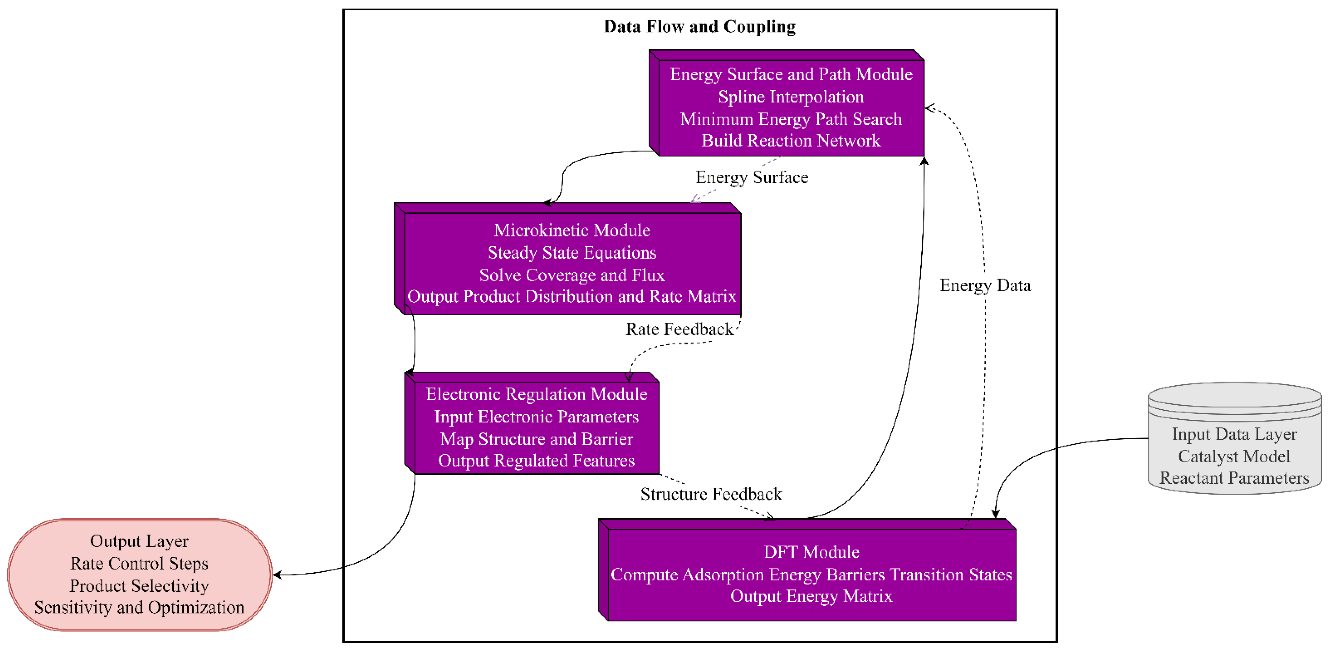
Numerical implementation details have a decisive influence on reproducibility. The numerical interface for DFT point-to-energy surface fitting uses a unified unit system and a reference state alignment strategy to eliminate zero-point offsets between different calculation batches. The unified reference state in this work is defined as setting the total energy of all isolated gas-phase molecules to zero electron volts. All adsorption energies and reaction energies for surface systems are calculated and compared using this zero reference. Energy values obtained from different calculation batches or different systems are aligned through this common reference to ensure consistency and comparability across the reaction path network. The Jacobian matrix of the steady-state algebraic equation is partially derived analytically to improve numerical stability, and the remaining terms are supplemented by adaptive differential approximations. Parallelization adopts a hybrid strategy of task parallelism (DFT point preprocessing) and data parallelism (multi-sample Monte Carlo) to leverage the benefits of modern computing resources. The output of the complete process includes the reaction path topology network, energy parameters and uncertainties for each step, steady-state coverage and path flux matrix, rate control metrics, and electronic state sensitivity maps to selectivity. The method framework diagram provides a structural diagram centered on data flow and key mathematical interfaces, as shown in Figure 6. The arrows in Figure 6 represent the directional flow of data and feedback between different modules of the framework.

3.3.2. DFT Calculation Module

This module uses the PBE exchange-correlation functional in the generalized gradient approximation as its theoretical foundation and employs a pseudopotential plane wave method to discretize energy and force calculations. All density functional theory calculations in this module are performed using the Vienna Ab initio Simulation Package(VASP, version 6.3.2), an open-source software developed at the University of Vienna [29,30,31]. The projected augmented wave method implemented in this package is employed to describe the ion–electron interaction. Transition state searches and frequency analyses are conducted using the VTST toolset (version 3.0). These software packages have been widely validated in the field of heterogeneous catalysis. A periodic slab model was used for system construction with a basal plane thickness of four layers. The lateral dimensions of the slab were 8.5 Å × 8.5 Å lateral dimensions, corresponding to a three-by-three supercell. The underlying atomic positions remained fixed during geometric relaxation, while the surface layers were fully relaxed. A vacuum layer thickness of 15 Å was used to eliminate periodic image interactions, and a dipole correction was applied when the surface was asymmetric. The pseudopotentials were implemented using the Projected Operator Augmented Wave (PAW) formulation, with a plane wave cutoff of 450 eV. Brillouin zone integration was performed using a Monkhorst–Pack k-point grid of 3 × 3 × 1 or denser in the surface direction to ensure energy convergence to less than 10⁻⁵ eV. A force convergence threshold of 0.02 eV·Å⁻¹ was used. Spin polarization was enabled for adsorbates and open-shell intermediates that contained unpaired electrons. For transition metal–oxides, a DFT + U correction was applied to account for localized electrons in strongly correlated systems. The U value was obtained from literature and experimental calibration and was fixed in the calculations. The long-range dispersion interaction was investigated using a semi-empirical Grimme D3 correction to obtain a reasonable energy ranking of the adsorption configurations.

The definition of adsorption energy is given by the total energy difference of the system, which is expressed as shown in Formula (9). Negative values of adsorption energy represent exothermic adsorption:

$${\mathrm{E}}_{\mathrm{ads}} ={ \mathrm{E}}_{\mathrm{slab}+\mathrm{ads}} - {\mathrm{E}}_{\mathrm{slab}} - {\mathrm{E}}_{\mathrm{adsorbate}}$$

(9)

In Formula (9), $E_{\mathrm{slab}+\mathrm{ads}}$ is the total energy of the system (surface and adsorbate), $E_{\mathrm{slab}}$ is the total energy of the clean surface, and $E_{\mathrm{adsorbate}}$ is the total energy of the adsorbate in the gas phase or isolated molecular state. The transition state energy barrier is defined as the difference between the transition state energy and the initial state energy. The minimum energy path search was carried out using the hill climbing elastic band (CI-NEB) method to locate the climbing point of the reaction. The climbing image after relaxation is refined to a single imaginary frequency using the hybrid dimer method or frequency calculation. The activation energy is expressed as follows:

$${\mathrm{E}}_{\mathrm{a}} = {\mathrm{E}}_{\mathrm{TS}} - {\mathrm{E}}_{\mathrm{initial}}$$

(10)

In Formula (10), $E_{\mathrm{TS}}$ is the transition state total energy and $E_{\mathrm{initial}}$ is the starting state total energy. The confirmation of the transition state depends on the first imaginary frequency, and its vibration mode is along the reaction coordinate direction. The frequency calculation uses the finite difference method to solve the mass-weighted Hessian matrix and adopts the resonance approximation for the adsorption state vibration. The vibration mode number excludes the influence of translational and rotational degrees of freedom in the surface adsorption system and is treated according to the adsorption constraint condition.

Free energy correction plays a key role in the input data of microdynamics. Free energy is obtained by superimposing the zero-point energy and thermodynamic correction terms based on the electron energy. It is calculated according to the following relationship:

$$\mathrm{G}\left(\mathrm{T},\mathrm{p}\right) = {\mathrm{E}}_{\mathrm{DFT}} + \mathrm{ZPE} + \mathrm{\Delta }{\mathrm{H}}_{\mathrm{vib}}\left(\mathrm{T}\right) - \mathrm{TS}\left(\mathrm{T},\mathrm{p}\right)$$

(11)

In Formula (11), $E_{\mathrm{DFT}}$ is the static electron energy, $\mathrm{ZPE}$ is the zero-point vibration energy, $\mathrm{\Delta }{H}_{\mathrm{vib}}\left(T\right)$ is the vibration thermodynamic correction, and $S\left(T,p\right)$ is the system entropy. The chemical potential of gas phase molecules is corrected according to the ideal gas approximation, and the gas phase chemical potential is expressed as

$$\mu \left(\mathrm{T},\mathrm{p}\right)={\mu }^{\circ }\left(\mathrm{T},{\mathrm{p}}^{\circ }\right)+{\mathrm{k}}_{\mathrm{B}}\mathrm{T}\mathrm{l}\mathrm{n}{\displaystyle \frac{\mathrm{p}}{{\mathrm{p}}^{\circ }}}$$

(12)

In Formula (12), ${\mu }^{°}\left(T,p^{°}\right)$ is the chemical potential at standard pressure $p^{° }$= 1 bar, $k_{\mathrm{B}}$ is the Boltzmann constant, and $\mathrm{p}$ is the actual partial pressure. The adsorption free energy or the free energy change of the reaction step is used to construct the energy surface and serves as the basis for calculating the microscopic kinetic rate constant. The entropy of the adsorbate on the surface is calculated using the resonance approximation, accounting for only the vibrational contribution. Under this approximation, the translational and rotational degrees of freedom of the surface adsorbate are completely frozen. The total entropy is obtained by summing the entropic contributions from all vibrational modes, each computed via standard statistical thermodynamic formulas using the mode frequency and temperature [32]. This treatment is justified for strongly chemisorbed systems where the adsorbate is confined to small vibrations around the adsorption site. The validity and error bounds of this approximation have been discussed in the surface thermodynamics literature [33]. The gas-phase molecular entropy is summed according to the rotational, translational, and vibrational degrees of freedom.

Transition state theory is used to derive microscopic rate constants from DFT data. Using transition state theory (TST) under the resonance approximation, the rate constant expression takes the following form:

$$\mathrm{k}\left(\mathrm{T}\right) = {\displaystyle \frac{{\mathrm{k}}_{\mathrm{B}}\mathrm{T}}{\mathrm{h}}}\exp \left(-{\displaystyle \frac{\mathrm{\Delta }{\mathrm{G}}^{‡}\left(\mathrm{T}\right)}{{\mathrm{k}}_{\mathrm{B}}\mathrm{T}}}\right)$$

(13)

In Formula (13), ${\mathrm{k}}_B$ is the Boltzmann constant, $\mathrm{h}$ is the Planck constant, and $\mathrm{\Delta }{G}^{‡}\left(T\right)$ is the activation free energy difference consisting of the DFT energy and vibrational terms. The frequency ratio of the pre-exponential term can be estimated by the product ratio of the reactant and transition state vibrational modes and further calibrated as the A factor in the microdynamics module. The frequency spectrum truncation and numerical stability are strictly checked in the calculation to avoid the influence of imaginary frequency or zero frequency errors on the A factor.

The transition state identification workflow involves initializing the NEB profile, performing full relaxation of several intermediate images until the force convergence criterion is met, performing fine relaxation of the climbing image, and performing frequency analysis of the resulting transition configuration to verify the single imaginary frequency nature. The energies, zero-point energies, and free energy corrections at 298 K of the adsorption configuration and transition state are summarized to provide input for the subsequent energy surface fitting and microdynamics solution. The DFT energy parameters of the main reaction intermediates and transition states are summarized in

Table 4. Energy parameters (all energy values are in units of electron volts).

Species/State	$E_{\mathrm{DFT}}$	ZPE	$G_{298\mathrm{K}}$	Remark
CO2(g)	0.00	0.00	0.00	Gas-phase reference
CO2*	−0.42	0.07	−0.35	Adsorbed state
COOH*	−0.85	0.12	−0.65	Intermediate
CO*	−0.32	0.04	−0.25	Adsorbed state
H*	−0.28	0.12	−0.10	Adsorbed state
CHO*	−0.70	0.08	−0.55	Intermediate
$T{S}_{C–C}$	1.22	0.05	1.15	C–C coupling transition state
$T{S}_{H\text{-}trans}$	0.95	0.04	0.88	Hydrogen transfer transition state

.

As shown in the table, all energies were corrected by zero-point energy and thermodynamics and processed using a unified reference state when constructing the reaction energy surface. The subsequent energy surface fitting and microdynamic solution used the free energy terms in the table as direct input to ensure the consistency between the kinetic parameters and the thermodynamic potential.

3.3.3. Energy Surface Fitting and Reaction Path Construction Module

This module takes a discrete first principles (DFT) energy point set ${({\xi }_k,{\eta }_k,E_k)}_{k=1}^N$ as input. The goal is to construct a smooth and physically constrained continuous energy field on the reaction coordinate plane $\hat{E}(\xi ,\eta )$ and identify the minimum energy path (MEP) and saddle point positions on this energy field to obtain the energy barriers and path topology of each key reaction step. The discrete points are mapped to a continuous field using a cubic B-spline basis expansion. The energy field is represented as

$$\begin{array}{c}\begin{array}{c}\hat{\mathrm{E}}(\xi ,\eta )=\sum _{\mathrm{i}=0}^{\mathrm{m}} \sum _{\mathrm{j}=0}^{\mathrm{n}} {\mathrm{c}}_{\mathrm{ij}}{\mathrm{B}}_{\mathrm{i}}^3(\xi ){\mathrm{B}}_{\mathrm{j}}^3(\eta )\end{array}\end{array}$$

(14)

In Formula (14), $B_i^3(\xi )$ and $B_j^3(\eta )$ are cubic B-spline basis functions, the coefficient $c_{\mathrm{ij}}$ is the fitting weight to be determined, and $\mathrm{m}$ and $\mathrm{n}$ are the upper limits of the basis function indices; the coordinates $\xi$ and $\eta$ are parameterized variables along the two orthogonal collective reaction coordinates, with $\hat{E}(\xi ,\eta )$ representing the fitting energy values at the corresponding coordinates. The fitting coefficients are obtained by solving the regularized least-squares problem, i.e., solving

$$\begin{array}{c}\underset{({\mathrm{c}}_{\mathrm{ij}})}{\min }\sum _{\mathrm{k}=1}^{\mathrm{N}}({\mathrm{E}}_{\mathrm{k}}-\hat{\mathrm{E}}({\xi }_{\mathrm{k}},{\eta }_{\mathrm{k}}){)}^2+\lambda {\int }_{\mathrm{\Omega }}|{\nabla }^2\hat{\mathrm{E}}(\xi ,\eta ){|}^2\mathrm{d}\xi \mathrm{d}\eta \end{array}$$

(15)

In Formula (15), $E_k$ is the energy sample obtained by DFT calculation $k$, $\lambda$ is the regularization parameter used to suppress overfitting and ensure the physical smoothness of the energy surface, ${\nabla }^2$ represents the Laplace operator, and the integration interval $\mathrm{\Omega }$ is the reaction coordinate domain. The regularization term is introduced in the discretized linear equations in the form of a Laplace matrix. The coefficients are solved using a sparse linear algebra solver constructed with node vectors, and the optimal value is determined by the generalized cross-validation of $\lambda$ to balance the approximation accuracy and surface smoothness.

After the energy surface is obtained, the initial path is established according to the arc length parameterization and the minimum energy path search is performed. The adaptive string method is used to evolve the path nodes to approximate the MEP. The node force is updated only along the energy gradient component perpendicular to the path direction according to the projection method. The node force is expressed as

$$\begin{array}{c}\begin{array}{c}{\mathrm{F}}_{\mathrm{i}}^{\perp }=-\nabla \hat{\mathrm{E}}({\mathrm{r}}_{\mathrm{i}})+(\nabla \hat{\mathrm{E}}({\mathrm{r}}_{\mathrm{i}})\cdot {\mathrm{t}}_{\mathrm{i}}){\mathrm{t}}_{\mathrm{i}}\end{array}\end{array}$$

(16)

In Formula (16), ${\mathrm{r}}_i = \left({\xi }_i,{\eta }_i\right)$is the $i$th coordinate vector of the node of the path, $\nabla \hat{E}({\mathrm{r}}_i)$ is the gradient of the energy field at ${\mathrm{t}}_i$, ${\mathrm{r}}_i$ is the unit tangent vector of the path at this node, and the dot product term is the projection of the gradient in the direction of the tangent vector. This projection is deducted from the total gradient to ensure that the node moves only in the direction perpendicular to the tangent vector. The node iterative update uses explicit time stepping:

$$\begin{array}{c}{\mathrm{r}}_{\mathrm{i}}^{\mathrm{n}+1} = {\mathrm{r}}_{\mathrm{i}}^{\mathrm{n}} + \mathrm{\Delta }\tau {\mathrm{F}}_{\mathrm{i}}^{\perp }\end{array}$$

(17)

As shown in Formula (17), $\mathrm{\Delta }\tau$ is the time step parameter. During the iteration process, the path is periodically reparameterized with equal arc length to maintain uniform node distribution and improve numerical stability. The mathematical foundation and convergence properties of the cubic B-spline fitting technique used to construct the continuous energy surface from discrete DFT points are detailed in the numerical analysis literature. The adaptive string method for minimum energy path search follows the standard algorithm described in previous methodological works. The spring constant used in the CI-NEB calculation was set to 5 eV/Ų. [34]. Each numerical subroutine has been independently programmed and verified against benchmark systems. After the adaptive string method converges, the highest energy image is refined by Climbing-Image Nudged Elastic Band (CI-NEB) to accurately locate the saddle point and obtain a reliable transition state energy barrier. The total force of each image in CI-NEB is given by the sum of the vertical component of the true force and the spring force along the tangential direction. The spring force is expressed as

$$\begin{array}{c}\begin{array}{c}{\mathrm{F}}_{\mathrm{i}}^{\mathrm{NEB}}=-\nabla \hat{\mathrm{E}}({\mathrm{r}}_{\mathrm{i}}){|}_{\perp }+\mathrm{k}(|{\mathrm{r}}_{\mathrm{i}+1} - {\mathrm{r}}_{\mathrm{i}}| - |{\mathrm{r}}_{\mathrm{i}} - {\mathrm{r}}_{\mathrm{i}-1}|){\mathrm{t}}_{\mathrm{i}}\end{array}\end{array}$$

(18)

In Formula (18), $-\nabla \hat{E}({\mathrm{r}}_i){|}_{\perp }$ indicates that the tangential component of the gradient has been removed to preserve the perpendicular component, $k$ is the spring constant, $|\cdot |$ represents the Euclidean distance between nodes, and ${\mathrm{t}}_i$ is the tangent vector. Used to constrain the spring force to the path direction, CI-NEB improves its climbing ability toward the saddle point by inverting the true force along the tangent direction of the highest energy image and removing the spring force, thereby converging to the precise transition state coordinates and energy values. 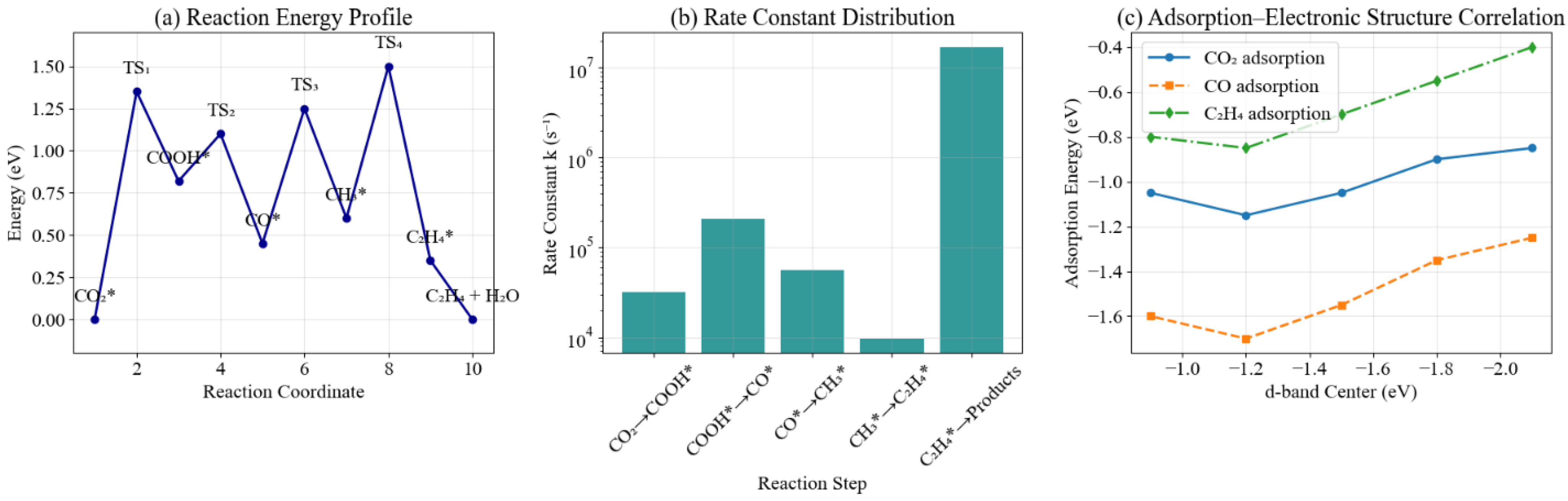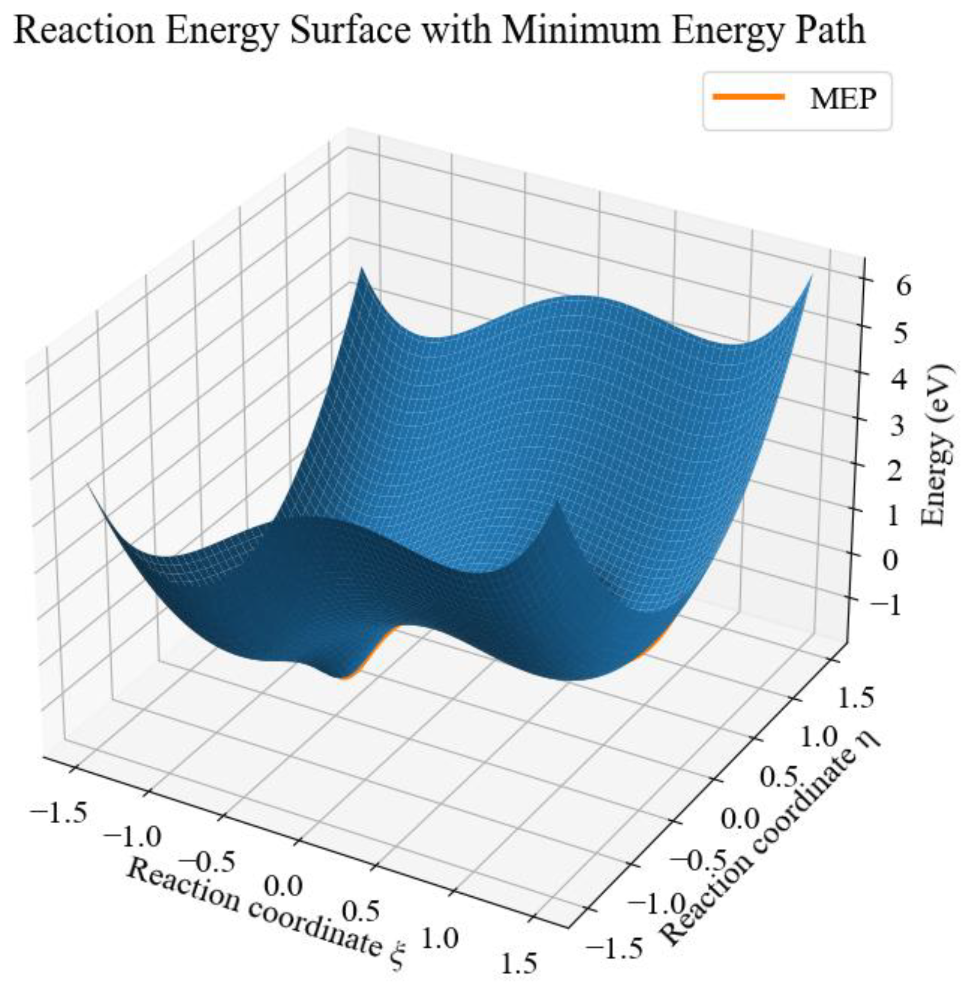The energy surface fitting process outputs a fitting coefficient matrix $c_{\mathit{ij}}$ and a smoothed residual distribution, while the path search outputs a sequence of MEP node coordinates, the energy of each node $\hat{E}({\mathrm{r}}_i)$, and the identified saddle point coordinates and energy barrier heights. These results provide quantitative parameters for the subsequent microdynamic solution module and are used for the precise calculation of rate constants. The fitted continuous energy surface and the identified minimum energy path are shown in Figure 7.

3.3.4. Microdynamics Solution Module

This section describes the solution process and mathematical expression from energy parameters obtained from first-principles calculations to the quantification of macroscopic reaction performance, clarifying the physical origin of the rate constant, the construction of the steady-state equation, and the method for determining the rate-controlling step. The rate constant adopts both the empirical Arrhenius expression and the rigorous expression of transition state theory to maintain an intuitive correspondence with the DFT free energy. The Arrhenius expression is given in Section 2.1, Formula (1). Transition state theory provides a microscopically comparable expression for the rate constant, given as Formula (2) in Section 2.1. To avoid linear algebraic pathology, the calculations screen the vibrational modes through symmetric coordinate transformations and implement truncation or statistical processing on low-frequency modes to ensure the numerical stability of the calculated prefactor $A_i$ and the activation free energy $\mathrm{\Delta }{G}_i^{‡}$.

Based on the microscopic reversible element reaction, the single-step reaction rate is given in the form of mass action law, and Formula (19) is expressed as

$$\begin{array}{c}{\mathrm{r}}_{\mathrm{j}}={\mathrm{k}}_{\mathrm{j}}^{+}\prod _{\mathrm{m}} {\mathrm{\theta }}_{\mathrm{m}}^{{\nu }_{\mathrm{m},\mathrm{j}}^{+}} - {\mathrm{k}}_{\mathrm{j}}^{-}\prod _{\mathrm{m}} {\mathrm{\theta }}_{\mathrm{m}}^{{\nu }_{\mathrm{m},\mathrm{j}}^{-}}\end{array}$$

(19)

In Formula (19), $r_j$ is the $j$th net rate of the element step (positive value means away from the adsorbate side); $k_j^{+}$ and $k_j^{-}$ are the forward and reverse rate constants, respectively; ${\theta }_m$ is the occupancy of the surface species $m$; and ${\nu }_{m,j}^{+}$ and ${\nu }_{\mathrm{m},\mathrm{j}}^{-}$ are the stoichiometric indices when the species acts as a reactant or product in the step. Surface site conservation is given as

$$\begin{array}{c}\sum _{\mathrm{m}} {\sigma }_{\mathrm{m}}{\mathrm{\theta }}_{\mathrm{m}}={\mathrm{\Theta }}_{\mathrm{tot}}\end{array}$$

(20)

In Formula (20), ${\sigma }_m$ is the number of sites occupied by the species ${\mathrm{\Theta }}_{\mathrm{tot}}$, $m$ is the total number of effective sites (calibrated to 1 in the model for simplicity), and the intermediates with multi-site occupation ${\sigma }_m > 1$ are directly reflected in the equation.

The steady-state approximation establishes a nonlinear algebraic equation system with the time derivative of the concentration of atoms/adsorbed intermediates equal to zero, which can be written in matrix form as follows:

$$\begin{array}{c}\mathrm{N}\cdot \mathrm{r}\left(\mathrm{\theta }\right) = 0\end{array}$$

(21)

In Equation (21), the matrix $\mathrm{N}$’s elements are the stoichiometric coefficients of each intermediate at each step, the vector $\mathrm{r}$ contains the net rate functions arranged by step, and the unknowns are given in the species occupancy vector $\theta$. This nonlinear system of equations is solved using the Newton–trust-region method, and the Jacobian matrix is explicitly constructed at each iteration to ensure convergence. The construction of the Jacobian matrix, step size control, and convergence criteria in this solver follow standard numerical algorithms documented in chemical kinetics literature. Initial guesses for steady-state coverages are obtained from Langmuir adsorption isotherm approximations [35], and a logarithmic transformation is applied to map coverage variables into an unconstrained space to improve numerical conditioning. Achieving a sustainable carbon-neutral economy necessitates the synergistic integration of advanced carbon capture technologies and renewable energy systems. Efficient CO₂ capture and separation materials provide the essential feedstock for downstream conversion [36], while the deployment of compressed carbon dioxide energy storage technologies offers a viable strategy for managing the intermittency of renewable power in green-hydrogen-enabled scenarios [37]. Within this ‘Power-to-X’ framework, the selective hydrogenation of CO₂ to light olefins hinges on the precise structural control of catalysts. Recent advancements in electronic structure regulation, particularly those demonstrated in copper-based systems for CO₂ reduction, emphasize that tailoring the surface adsorption environment is key to governing intermediate stabilization and achieving high product selectivity [38]. To improve robustness to the initial guess, physical constraints are imposed on the minimum and maximum occupancies during the iterations $\left[0,1\right]$, and the occupancies are processed using a logarithmic transformation to reduce numerical rigidity. After the steady-state solution is derived, the overall yield and selectivity of the system are obtained by integrating the surface desorption rates of each path, and the conversion is calculated as the difference in the feed-discharge molar flow.

Reaction rate control analysis uses a sensitivity matrix and the degree of rate control (DRC) metric. The DRC is defined as the logarithmic derivative of the target reaction rate with respect to a perturbation of the rate constant, as shown in the following form:

$$\begin{array}{c}{\mathrm{X}}_{\mathrm{i}} = {\displaystyle \frac{\partial \ln {\mathrm{r}}_{\mathrm{tot}}}{\partial \ln {\mathrm{k}}_{\mathrm{i}}}}{|}_{\mathrm{T},\mathrm{P}} = {\displaystyle \frac{{\mathrm{k}}_{\mathrm{i}}}{{\mathrm{r}}_{\mathrm{tot}}}}{\displaystyle \frac{\partial {\mathrm{r}}_{\mathrm{tot}}}{\partial {\mathrm{k}}_{\mathrm{i}}}}{|}_{\mathrm{T},\mathrm{P}}\end{array}$$

(22)

In Formula (22), $r_{\mathrm{tot}}$ is the evaluation target (e.g., the steady-state production rate of light olefins) and the sign and magnitude of $X_i$ directly reflect the amplification or suppression effect of the step on the overall rate. The characterization obtained by DRC is used to calculate the path decomposition of the apparent activation energy $E_{\mathrm{app}}$, expressed as Formula (23):

$$\begin{array}{c}{\mathrm{E}}_{\mathrm{app}} = \sum _{\mathrm{i}} {\mathrm{X}}_{\mathrm{i}}{\mathrm{E}}_{\mathrm{i}}\end{array}$$

(23)

In Formula (23), $E_i$ is the $i$th activation energy of the step (eV). This decomposition provides a direct quantitative explanation of the temperature sensitivity and rate determining factors from the perspective of energy barriers.

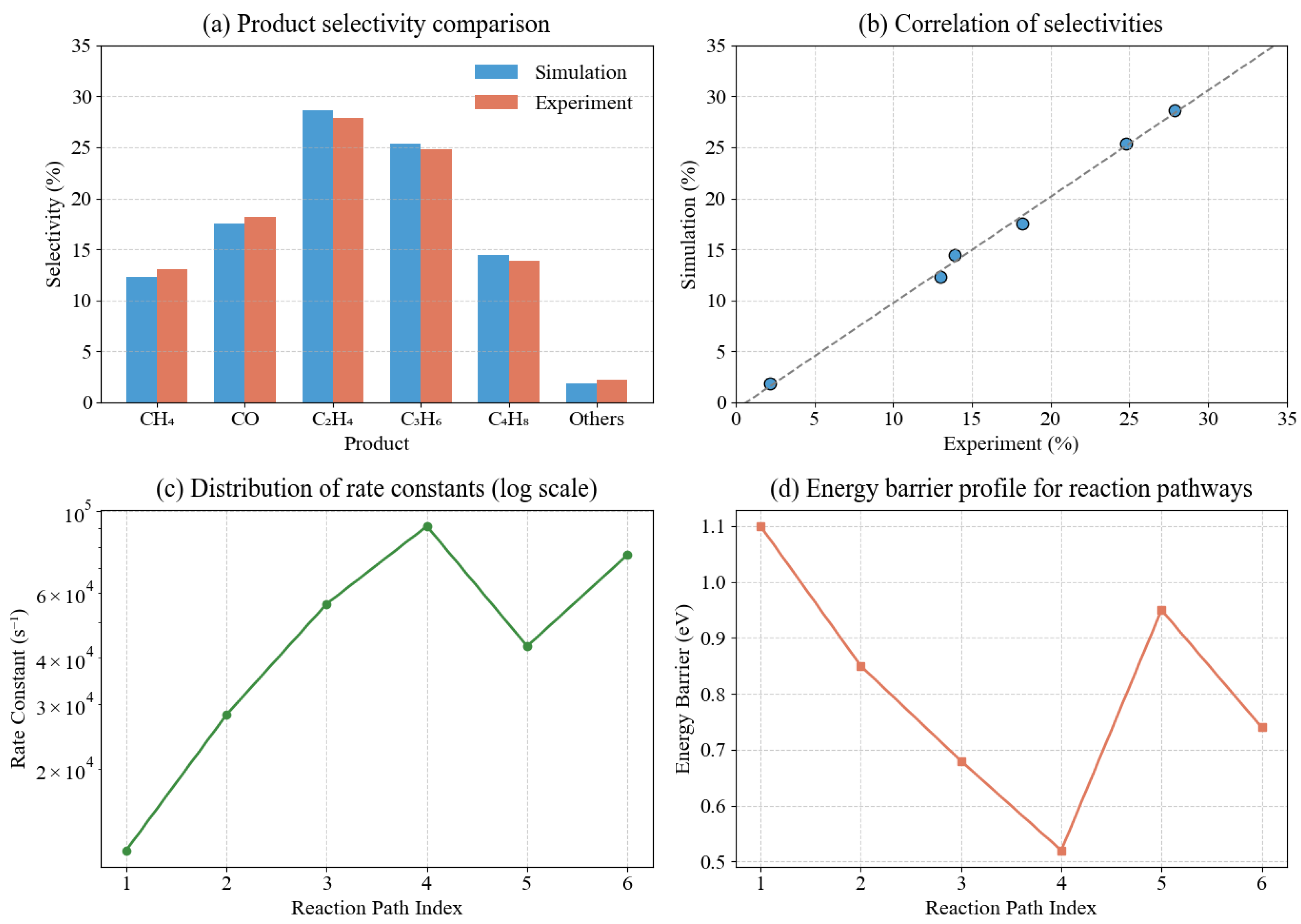
The boundary conditions and local interactions of the steady-state mean-field solution were verified using a parallel lattice-based Monte Carlo (lattice kMC) algorithm. Grid kMC uses event rates generated by Equation (2) under the same energy parameter set. Events included adsorption/desorption, surface migration, hydrogen transfer, and C–C coupling. The event frequency distribution output by kMC was used as a correction factor to adjust the ligand/coverage dependence in the mean-field model, which eliminated bias in the mean-field under strong coverage or ordered adsorption. The TOF (turnover frequency) and product selectivity obtained by the two methods were compared to assess the model uncertainty and define parameter sensitivity ranges.

The numerical implementation details adopt a modular structure: the rate constant table was generated by the DFT energy barrier and transition state vibrational data preprocessing module; the steady-state solution module used a sparse Jacobian construction and a parallel linear algebra solver to handle large-scale reaction networks; and the sensitivity analysis module used a dual-track parallel calculation based on finite differences and automatic differentiation to ensure the accuracy of sensitivity gradients and reduce numerical noise. After the solution was found, parameter sweeps of the temperature, pressure, and ratio were performed to obtain a global response surface of steady-state rate matrices and product distributions, which served as input for subsequent structure control mapping.

To clearly present the core information of the model output, a concise summary table is provided for the forward and reverse rate constants and the corresponding steady-state surface occupancies of the key reaction pathways. The rate constants reported in

Table 5. Rate constants and steady-state coverage.

Step Label	${\mathit{k}}^{\mathbf{+}}\mathbf{(}{\mathbf{s}}^{\mathbf{-}\mathbf{1}}\mathbf{,} \mathbf{573} \mathbf{K}\mathbf{)}$	${\mathit{k}}^{\mathbf{-}}\mathbf{(}{\mathbf{s}}^{\mathbf{-}\mathbf{1}}\mathbf{,} \mathbf{573} \mathbf{K}\mathbf{)}$	Steady-State Coverage ($\mathit{\theta }$)
CO2 adsorption/activation	$1.2 \times {10}^2$	$4.0 \times {10}^{-1}$	0.18
Intermediate hydrogenation	$3.5 \times {10}^1$	$2.1 \times {10}^{-2}$	0.12
CO formation/desorption	$6.8 \times {10}^0$	$1.0 \times {10}^{-3}$	0.05
C–C coupling	$9.0 \times {10}^{-1}$	$2.5 \times {10}^{-4}$	0.07
Olefin desorption	$2.4 \times {10}^1$	$8.2 \times {10}^{-3}$	0.04

are evaluated at the model reference temperature of 573 K and are expressed in units of s⁻¹. Each occupancy represents a dimensionless surface coverage fraction.

3.3.5. Electronic Structure Control and Structural Parameter Mapping

This section establishes a quantitative mapping from catalyst geometry and chemical structure parameters to local electronic state variables, as well as an analytical relationship from electronic state variables to intermediate adsorption energy and reaction energy barriers, and then substitutes these relationships into microscopic kinetic expressions to obtain the direct control law of structural parameters on the rate of key reaction steps. The local electronic state of the catalyst surface is characterized by the d-band center (denoted as ${\epsilon }_{\mathrm{d} }$) and the local state density gradient, and the structural parameters are input variables with the surface coordination number (CN), lattice strain (strain, denoted as (s)) and alloy component mole fraction (composition fraction, denoted as (x)). The linear regression model from the geometric and chemical parameters to d-band center adopts the following form [29]:

$${\epsilon }_{\mathrm{d}} = {\mathrm{c}}_0 + {\mathrm{c}}_1{\displaystyle \frac{1}{\mathrm{CN}}} + {\mathrm{c}}_2\mathrm{s} + {\mathrm{c}}_3\mathrm{x}$$

(24)

In Formula (24), the variable on the left ${\epsilon }_d$ is the $d$-band center; the constant term on the right $c_0$ is the baseline $d$-band center; the term $\mathrm{CN}$ represents the upward shift of the local energy level caused by low coordination; the coefficient $c_1$ is the sensitivity coefficient, whose sign and dimension reflect the directional effect of coordination change on the energy band; $s$ is the lattice strain (positive value is tension, negative value is compression); the coefficient $c_2$ represents the modulation sensitivity of strain on electronic structure; $x$ is the mole fraction of the alloy guest component; and the coefficient $c_3$ represents the chemical shift effect of the chemical component on the $d$-band center. The model used a set of catalyst structure samples obtained by DFT calculation as training data. A weighted least-squares fit was used to obtain the coefficient matrix $\left\{c_i\right\}$ and evaluate the fitting confidence interval and determination coefficient to ensure that the changes in structural parameters can be quantitatively described by the electronic state.

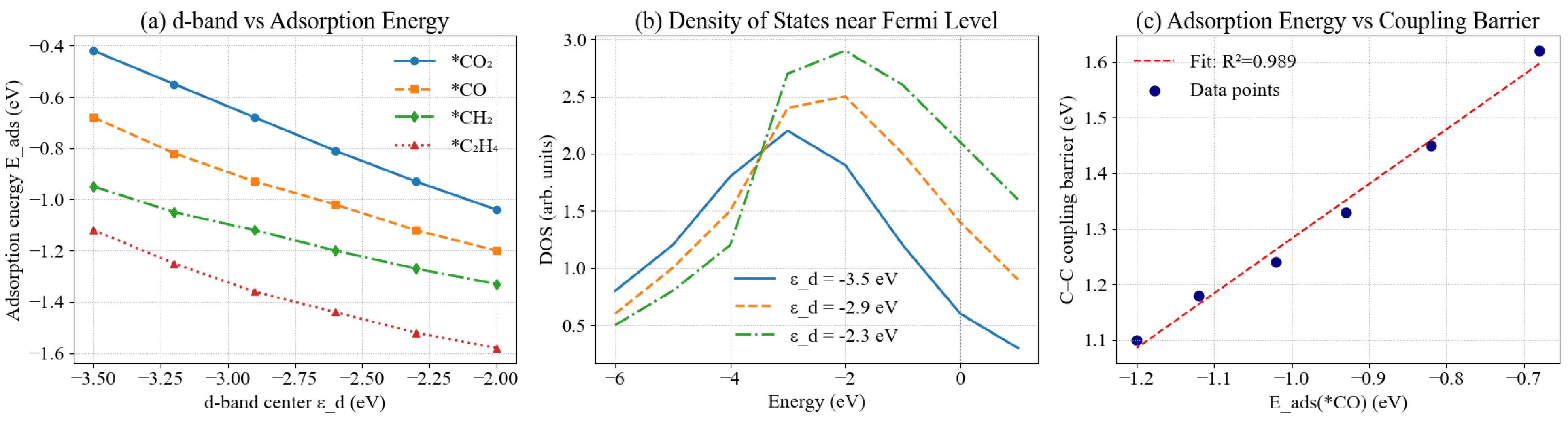
To describe the relationship between the electronic state and the intermediate adsorption energy, as well as the coupling between adsorption energy and activation energy, a linear Brønsted–Evans–Polanyi (BEP)-type approximation and a linear d-band-center relation are adopted. The change in adsorption energy relative to the baseline value is denoted as $\mathrm{\Delta }{E}_{\mathrm{a}\mathrm{d}\mathrm{s}}$, and its dependence on the d-band center is expressed as follows:

$$\mathrm{\Delta }{\mathrm{E}}_{\mathrm{ads}} = \mathrm{m}\left({\epsilon }_{\mathrm{d}} - {\epsilon }_{\mathrm{ref}}\right) + \mathrm{n}$$

(25)

In Formula (25), $\mathrm{\Delta }{E}_{\mathrm{ads}}$ is the change in the adsorption energy of the intermediate $m$ on a given surface relative to a reference surface (with the band center at $d$). The coefficient ${\epsilon }_{\mathrm{ref}}$ represents the sensitivity of the adsorption energy due to the shift in the $d$-band center and is often negative to reflect the physical trend of enhanced adsorption due to an upward shift in the $d$-band center. The constant $n$ is the inherent deviation term of the system. The change in adsorption energy is expressed in a linear BEP relationship with the activation energy of the corresponding reaction step:

$${\mathrm{E}}_{\mathrm{a}} = \mathrm{a}\mathrm{\Delta }{\mathrm{E}}_{\mathrm{ads}} + \mathrm{b}$$

(26)

In Formula (26), $E_{\mathrm{a}}$ is the activation energy of the reaction step; the parameter $\mathrm{a}$ is the BEP slope, which represents the transfer coefficient of the adsorption energy change to the activation energy; and the constant term $b$ is the reference activation energy under the reference adsorption energy condition. Substituting Formula (25) into Formula (26), the activation energy can be expressed explicitly as a function of the d-band center [30]:

$${\mathrm{E}}_{\mathrm{a}} = \mathrm{a}\left(\mathrm{m}\left({\epsilon }_{\mathrm{d}} - {\epsilon }_{\mathrm{ref}}\right) + \mathrm{n}\right) + \mathrm{b} = \left(\mathrm{am}\right){\epsilon }_{\mathrm{d}}+\left(\mathrm{b}-\mathrm{am}{\epsilon }_{\mathrm{ref}}+\mathrm{an}\right)$$

(27)

In Formula (27), the left-side $E_{\mathrm{a}}$ is the activation energy, the first coefficient on the right side $\mathrm{am}$ gives the direct linear increase/decrease flux of the activation energy due to the change in the $d$-band center, and the constant term in brackets is the baseline activation energy correction. Substituting this expression into the microkinetic rate expression, the rate constant adopts the Arrhenius form $k = A\exp (-E_{\mathrm{a}}/\mathrm{RT})$, and taking the derivative with respect to $\ln k$ obtains the parameter sensitivity formula, where ${\epsilon }_d$ quantifies the exponential amplification effect of a small shift in the $d$-band center on the step rate. The sensitivity expression is written as

$${\displaystyle \frac{\partial \ln \mathrm{k}}{\partial {\epsilon }_{\mathrm{d}}}}=-{\displaystyle \frac{\mathrm{am}}{\mathrm{RT}}}$$

(28)

In Formula (28), the left side represents the derivative of the natural logarithm of the rate constant with respect to the $d$-band center, while the parameters on the right side include temperature $T$, $\mathrm{am}$, and the gas constant $\mathrm{R}$. The product of the coefficients determines the direction and absolute value of the sensitivity; the positive and negative signs reflect the direction of rate enhancement or inhibition caused by an upward shift in the $\mathrm{d}$-band center. This sensitivity expression is used to identify the relative degree to which structural parameter changes amplify or inhibit the rates of each key step at a given reaction temperature and to translate structural design objectives into electronic state control targets, thereby achieving quantitative coupled control of the C–C coupling step and the hydrogen migration step.

To quantify the above mapping relationship and kinetic sensitivity, a dataset consisting of DFT samples was used to perform stepwise regression fitting on the Equations (24) to (27). The obtained fitting coefficients and statistical indices are listed in

Table 6. Electronic structure parameters and energy barrier mapping coefficients.

Parameter	Fitted Value	Unit	Description
$c_0$	−2.10	eV	Baseline d-band center
$c_1$	0.85	eV	Sensitivity to inverse coordination number
$c_2$	1.20	eV	Strain sensitivity (per 1% strain)
$c_3$	−0.65	eV	Sensitivity to alloy composition (mole fraction)
$m$	−0.78	eV/eV	Linear coefficient of d-band center vs. adsorption energy
$n$	0.02	eV	Adsorption energy offset term
$a$	0.62	–	BEP slope coefficient
$b$	0.92	eV	Reference activation energy
$R^2$	0.93	–	Goodness of fit for regression
RMSE	0.07	eV	Root-mean-square error

; the structural parameters can be directly input into the rate constant calculation module in the subsequent microscopic kinetic solution stage and the path contribution rate and selectivity distribution can be output.

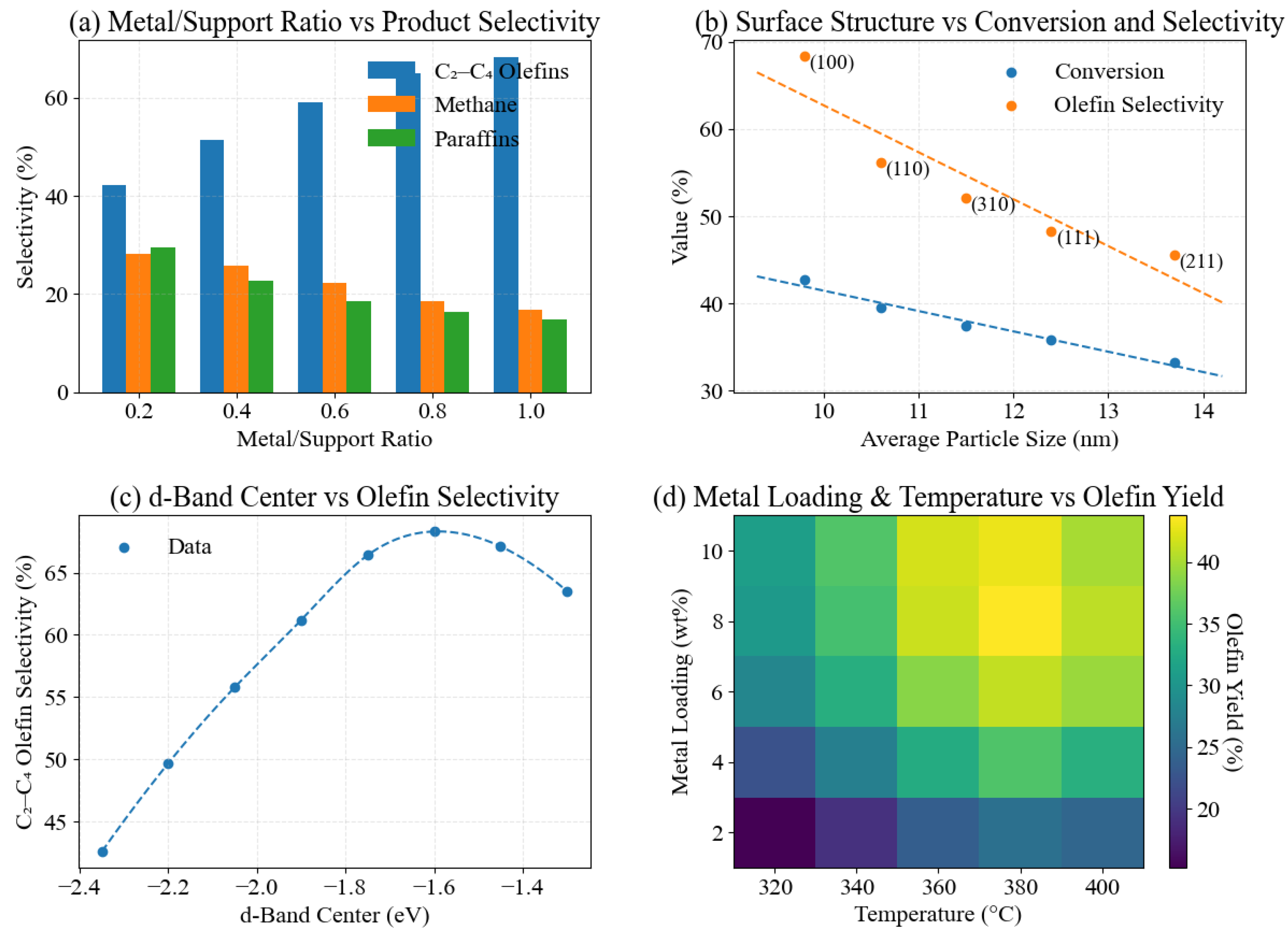
As shown in Table 6, these coefficients and statistics are directly fed into the microkinetics solver module and serve as part of the structural optimization objective function. This function searches within the design space for structural parameter combinations that maximize the activation energy difference for key steps (C–C coupling or hydrogen migration) and favor light olefin selectivity. This mapping relationship is then used in subsequent model validation and experimental comparison to quantitatively map structural indices obtained through XRD, XPS, and TEM into kinetic predictions, thereby achieving a closed-loop quantitative design process from structural preparation to product distribution.

4. Conclusions

By integrating first-principles microkinetic simulation (FPMS) with a high-fidelity reaction-pathway energy surface derived from DFT calculations, this study enables quantitative pathway analysis and elucidates the structural control mechanisms governing CO₂ hydrogenation to light olefins. Model–experiment comparison shows that the energy barrier for CO₂ adsorption to COOH* is 1.35 eV, whereas the transition-state barrier for C–C coupling is 1.50 eV, identifying C–C coupling as the key rate-limiting step. The corresponding reaction rate is only 9.7 × 10³ s⁻¹, in contrast to an olefin desorption rate of 1.7 × 10⁷ s⁻¹, underscoring pronounced differences in kinetic control across reaction stages. The model’s predictive fidelity was validated experimentally: the ethylene selectivity of 27.9% closely matches the simulated 28.6% (deviation < 1%), demonstrating reliable product-distribution forecasting. Moreover, electronic structure manipulation experiments reveal that shifting the d-band center from −2.35 eV to −1.60 eV increases the C₂–C₄ olefin selectivity from 42.6% to 68.3%, confirming the directional influence of electronic state modulation on pathway branching. Taken together, the proposed FPMS framework establishes a verifiable closed loop from energy-surface construction to product-distribution prediction, quantitatively mapping structural parameters and electronic states onto reaction kinetics. This approach offers substantial practical value for high-value CO₂ utilization and provides a systematic, mechanism-grounded basis for the rational design and optimization of highly selective light-olefin catalysts.