Article

Accelerating Kinetic Parameter Identification by Extracting Information from Transient Data: A Hydroprocessing Study Case

1
IFP Energies nouvelles, Rond-point de l’échangeur de Solaize, BP 3, 69360 Solaize, France
2
Laboratory for Chemical Technology, Ghent University, Technologiepark 125, B-9052 Ghent, Belgium
*
Author to whom correspondence should be addressed.
Catalysts 2020, 10(4), 361; https://doi.org/10.3390/catal10040361
Submission received: 25 February 2020 / Revised: 16 March 2020 / Accepted: 24 March 2020 / Published: 26 March 2020
(This article belongs to the Special Issue Catalyst Deactivation and Regeneration)

Abstract

:
Hydroprocessing reactions require several days to reach steady-state, leading to long experimentation times for collecting sufficient data for kinetic modeling purposes. The information contained in the transient data during the evolution toward the steady-state is, at present, not used for kinetic modeling since the stabilization behavior is not well understood. The present work aims at accelerating kinetic model construction by employing these transient data, provided that the stabilization can be adequately accounted for. A comparison between the model obtained against the steady-state data and the one after accounting for the transient information was carried out. It was demonstrated that by accounting for the stabilization, combined with an experimental design algorithm, a more robust and faster manner was obtained to identify kinetic parameters, which saves time and cost. An application was presented in hydrodenitrogenation, but the proposed methodology can be extended to any hydroprocessing reaction.

1. Introduction

A good prediction of overall process performance based on the input conditions is of great interest in many domains, especially in the chemical industry. In general, predictive models are usually trained on the experimental data, which can then interpolate well in a similar domain with the experimental data. However, extrapolation toward a new domain can be less reliable. Model recalibration is then required, which leads to a demand for new training data. Collecting data is usually expensive and time-consuming, hence, acquired data should be exploited in their entirety. Particularly for petroleum related conversion processes (e.g., hydrotreating and hydrocracking), it appears that available data are only partially used during modeling, see below. The challenge is, hence, to exploit the non-used data to uncover the underlying information and determine the model more rapidly and/or precisely.
Hydrotreating is a catalytic conversion process to remove heteroatoms such as sulfur, nitrogen, oxygen, and other impurities such as nickel and vanadium in hydrocarbon feedstocks. It is implemented in modern refineries to meet the post-refining process specifications for the intermediate products as well as the environmental regulations for the final products. Hydrocracking is a catalytic process converting diverse feedstocks such as gas oil, vacuum gas oil, deasphalted oil, and biomass-derived oils into more valuable products such as naphtha, kerosene, and diesel [1]. These processes play an important role in refineries. Since 1950, together with the development of the transportation industries, hydrocracking has become a promising technology to respond to the high demand for clean diesel in the road and railroad sector and for jet fuel in the aviation sector [2]. Furthermore, the availability of sufficient low cost hydrogen as a by-product from the catalytic reforming of naphtha was a key factor in the popularity of hydroprocessing. Nowadays, the interest in hydroprocessing is further increased thanks to governmental policies focusing on emissions reduction and energy efficiency. According to official statistics from Stratas Advisors [3], many countries among which those belonging to the EU, North America, Russia, China, and Australia limit the sulfur content in on-road diesel to 10–15 ppm, a limit that is progressively being adopted in all remaining countries. According to the International Maritime Organization (IMO), even the global limit of sulfur in bunker fuel will be reduced from 3.5% to a maximum of 0.5% m/m from January 2020 onward [4]. Low sulfur marine distillate is forecasted to displace high sulfur fuel oil.
A kinetic model is an essential tool for the adequate design and simulation of chemical processes [5]. Hydroprocessing kinetic modeling is a challenging and time-consuming task as the crude oils contain many compounds with complicated structures [6]. Diverse approaches for hydroprocessing modeling have been developed in the past such as the lumping technique [7,8,9,10,11,12], detailed kinetic modeling [13,14,15,16,17,18,19], and black-box approach [20,21,22,23]. The lumping technique, which consists of regrouping chemical compounds with similar properties, is the most common and widely used [24]. The common point in these approaches is that the model parameters are generally estimated by fitting the model to steady-state experimental data, even if the time to reach the steady-state in hydroprocessing experimentation can be excessively long. Yang et al. (1983) [25] demonstrated that, for hydrodenitrogenation over a NiMo/Al2O3 catalyst, the steady state was reached after around six to eight days depending on the operating conditions. Sau et al. (2005) [26] observed a steady state reached after eight days for hydrocracking experiments using the zeolite-based catalyst. The time to reach steady state is denoted as ‘stabilization’, which was recently the focus in our previous work [27]. It was found that the stabilization is mainly driven by chemical rather than hydrodynamic phenomena. It relates to changes in the state of the catalyst, which require up to several days, depending on the feedstock and the operating conditions.
The stabilization leads to long campaigns to obtain sufficient steady-state experimental data for kinetic modeling purposes. However, in the transient regime toward the steady state, effluent analyses are already carried out at regular time intervals in order to verify if the steady state has effectively been reached. These transient data are currently not used for kinetic modeling because no specific simulation model was available to describe this stabilization behavior. It is reported in the literature that using transient data saves time and cost when there is a significant gap between the time required to reach steady state and the analysis time [28], which is the case in hydroprocessing.
Hence, the aim of the present work was to employ transient data for kinetic model parameter determination in hydroprocessing. Hydrodenitrogenation was selected as a study case since it is a crucial reaction to remove organic nitrogen compounds, which are inhibitors for hydrocracking. Kinetic model parameters for hydrodenitrogenation were determined either from steady-state data or in conjunction with a description of the stabilization kinetics. The advantages of employing transient data were demonstrated via a quality comparison between the global model performance and individual parameter significance for both cases.

2. Results and Discussion

Experimental data using in this study was explained in Section 3.2. A model accounting for the stabilization behavior was integrated into the kinetic model, which is detailed in Section 3.3.1. Two approaches for kinetic parameter estimation: (1) using only steady-state data (i.e., steady-state kinetic model) and (2) using transient and steady-state data (i.e., model including stabilization) are compared. Section 2.1 exhibits the results of the comparison by applying the strategy described in Section 3.3.3. Section 2.2 performs the robustness of employing transient data with a procedure detailed in Section 3.3.4.

2.1. Model Including Stabilization vs. Steady-State Model

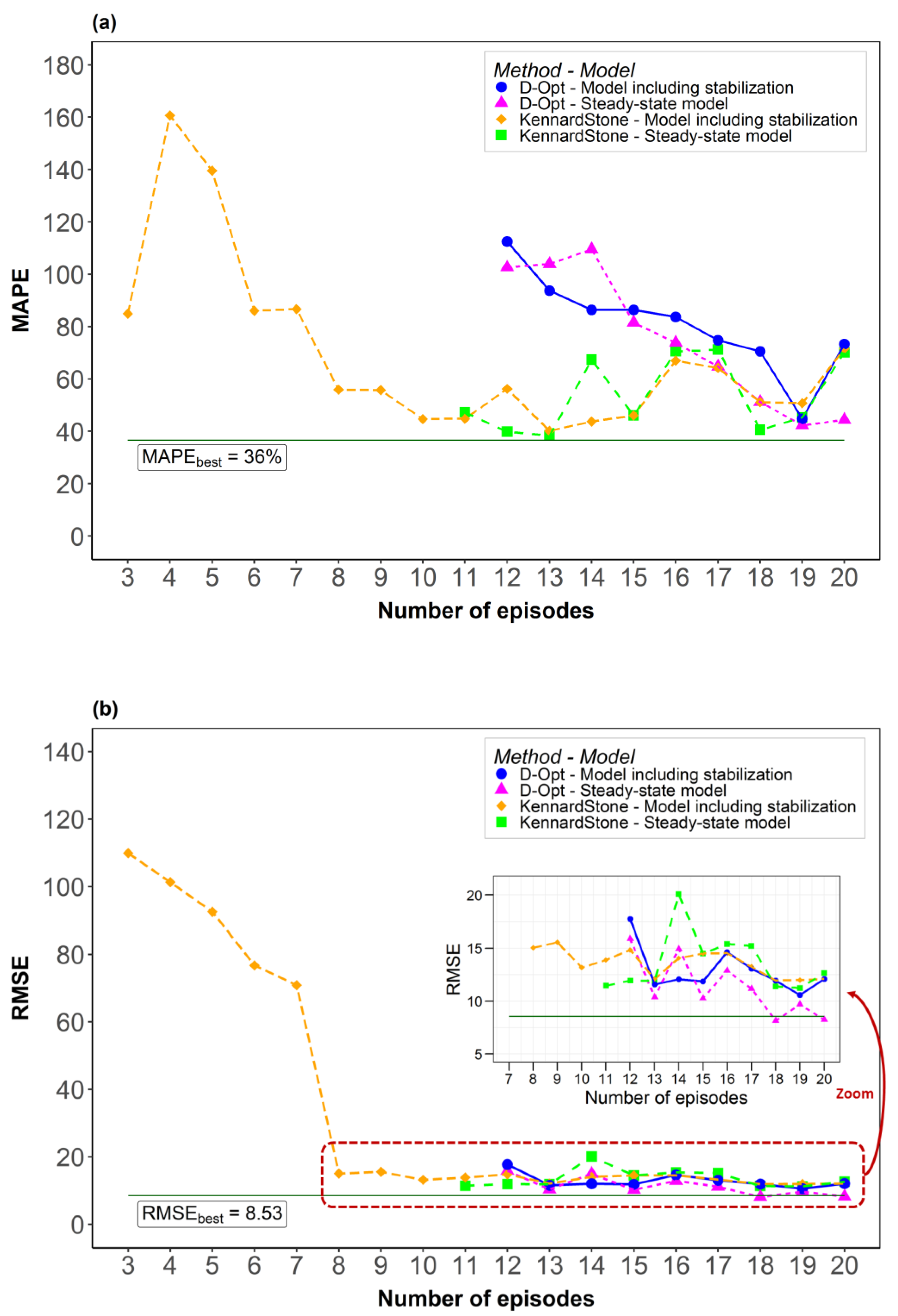
The best estimates for the kinetic model parameters are believed to be obtained when all of the 38 steady-state measurements were used to fit the hydrodenitrogenation kinetic model. Figure 1 displays the parity diagram for fitting the hydrodenitrogenation against all available 38 steady-state points. It is considered as the reference scenario, since all the steady-state points are exploited to estimate the kinetic parameters. The quality indicator mean absolute percentage error (MAPE) and root mean square error (RMSE) on the entire steady-state points amounted to 36.63% and 8.53, respectively.
The model performance comparison with the parameters being determined against steady-state data only or the data including stabilization is shown in Figure 2. The indicators were calculated on all 38 steady-state points. The impact of the number of episodes in the calibration database was analyzed by comparing the model performance with the obtained parameter estimates to the reference scenario. When employing the Kennard–Stone algorithm, the minimum number of selected episodes in the calibration dataset is 2, corresponding to 10 experimental data points. However, it is impossible to fit the model including stabilization with only two episodes since the number of parameters in the kinetic model employing transient data amounts to 13 (i.e., 11 kinetic parameters and two transient parameters). Hence, the minimum was three in this study. Apart from that, when using steady-state data only, the kinetic parameters can only be calibrated using at least 11 steady-state points (of 11 episodes). It explains why in Figure 2, the performance indicators for parameter estimates determined from transient data determined according to Kennard–Stone already appeared at the number of episodes in the calibration database between 3 to 10. D-optimal design was used for the determination of the kinetic parameters. As explained in Section 3.3.3, the minimum number of selected episodes was 12 (number of parameters + 1) to allow for the determination of all the parameters including the statistics. Note that the episodes selected by Kennard–Stone and D-optimal can be different. As can be seen, for each comparison, the prediction performance of the model parameters obtained with the data accounting for stabilization was similar to that with the model parameters determined against the steady-state data only.
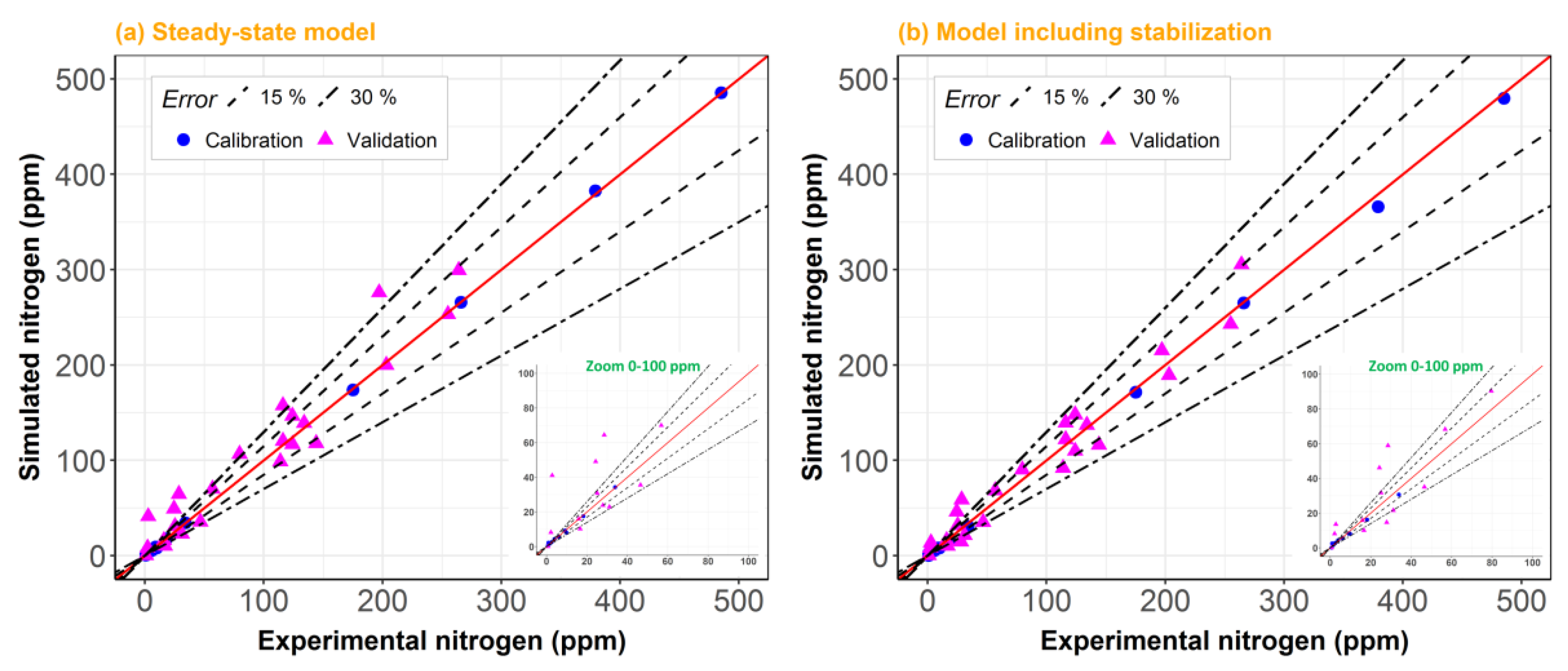
As can be seen, one of the main advantages of accounting for stabilization is that thanks to transient points, it becomes possible to calibrate the model with a lower number of experiments. The Kennard–Stone algorithm is very competitive with the D-optimal design in this study. Figure 2 shows that the accuracy was similar for both cases. An example of the parity plot comparison in the case of a calibration database containing 14 episodes selected by the Kennard–Stone technique is given in Figure 3. Using transient data to determine the model parameter estimates (Figure 3b) led to a slightly better prediction accuracy than when using the steady-state data only (Figure 3a).
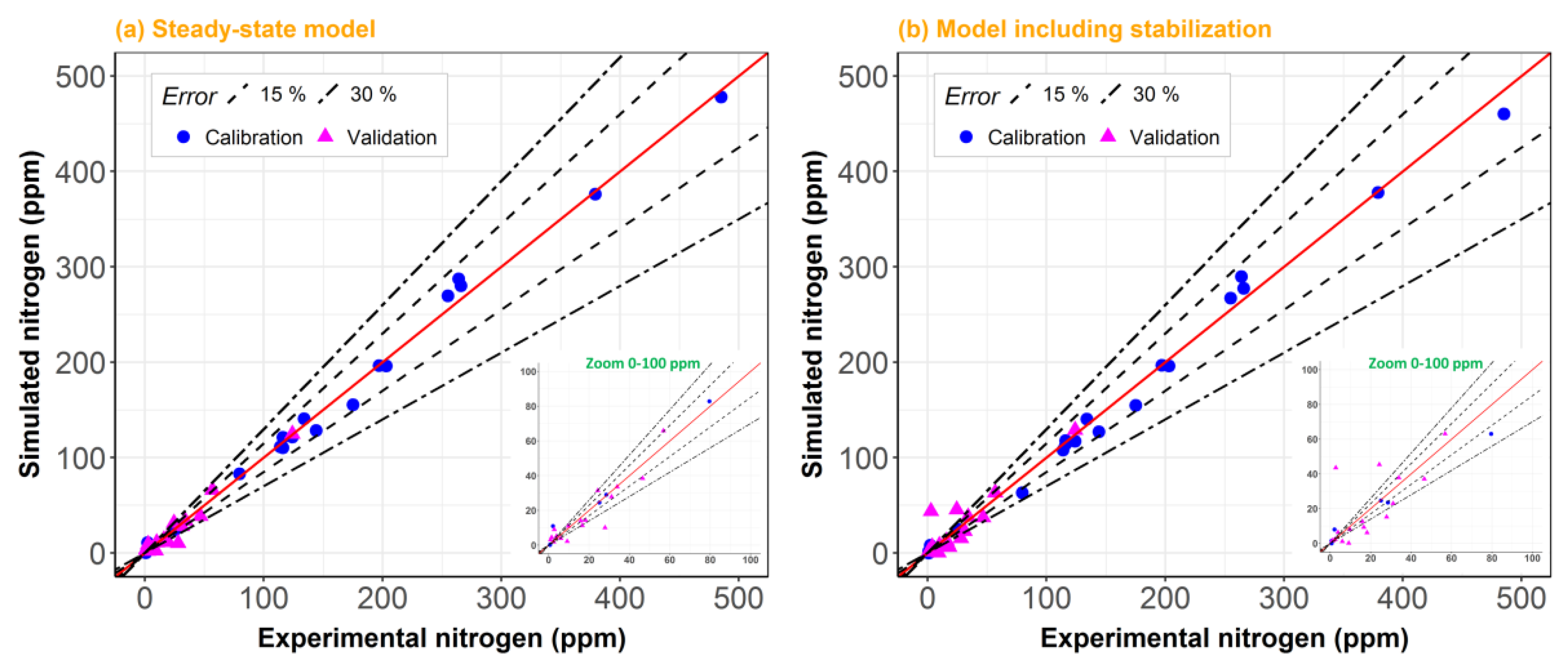
In the case of a calibration database containing 20 episodes selected by the D-optimal design, the accuracy of the model including stabilization was similar to the steady-state model. The parity plots are detailed in Figure 4.
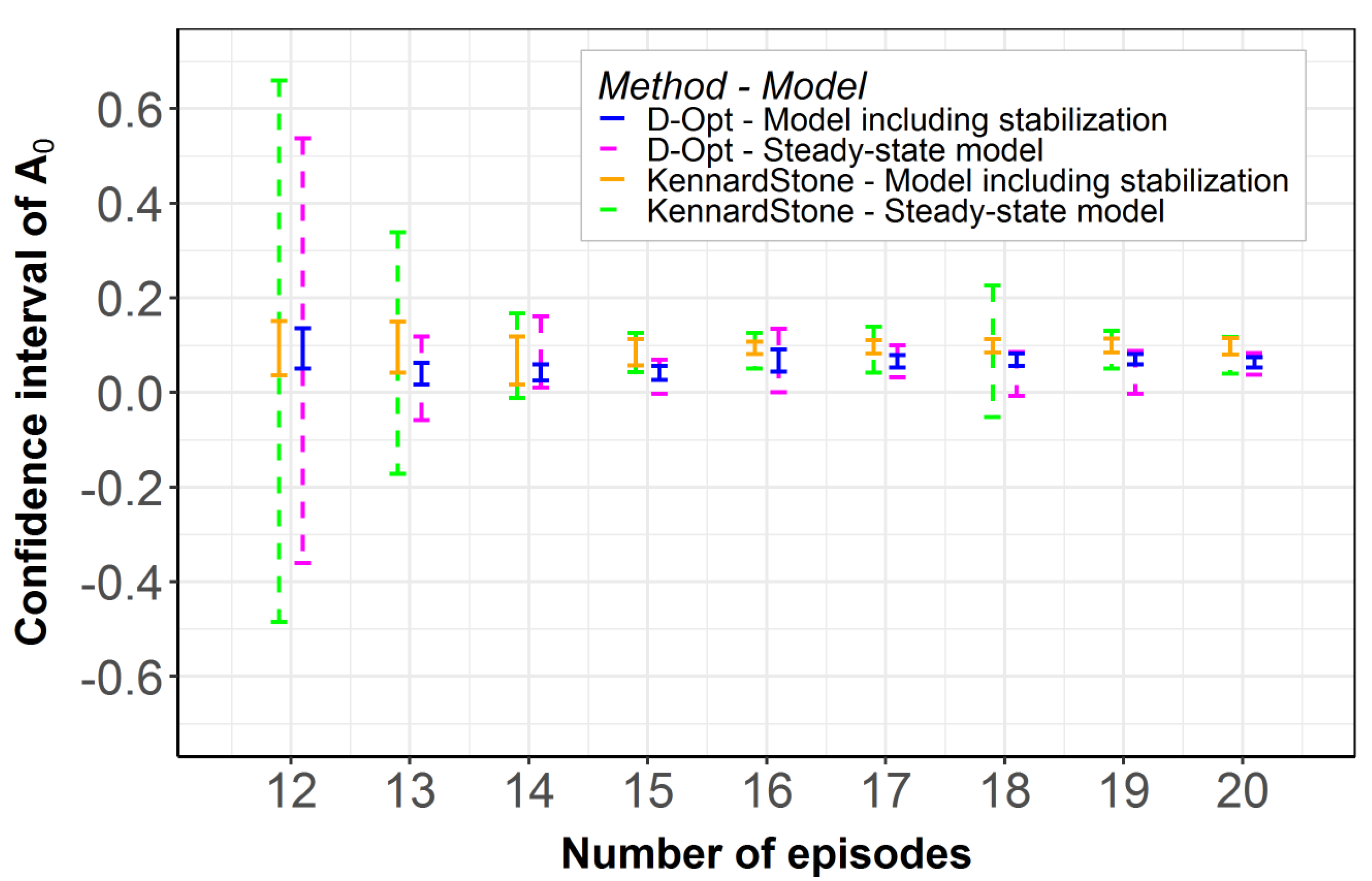
Parameter estimates determined from data including stabilization had the same order of magnitude as the ones determined from the steady-state data only. More narrow confidence intervals were obtained in the former case. Regarding the technique of selecting episodes, parameter estimates obtained when using the D-optimal and Kennard–Stone technique were similar. An example of the confidence intervals of the resin adsorption coefficient (parameter A0) is shown in Figure 5. The pink dashed line and blue solid line represent the confidence interval in the case of steady-state data only and data including stabilization, respectively, in the D-optimal technique. In the Kennard–Stone case, it was shown as the green dashed line and orange solid line. Irrespective of the number of episodes used, a more narrow confidence interval was obtained by employing transient data. Figure 5 also nicely demonstrates how the confidence also becomes narrower with the number of episodes considered in the calibration dataset.
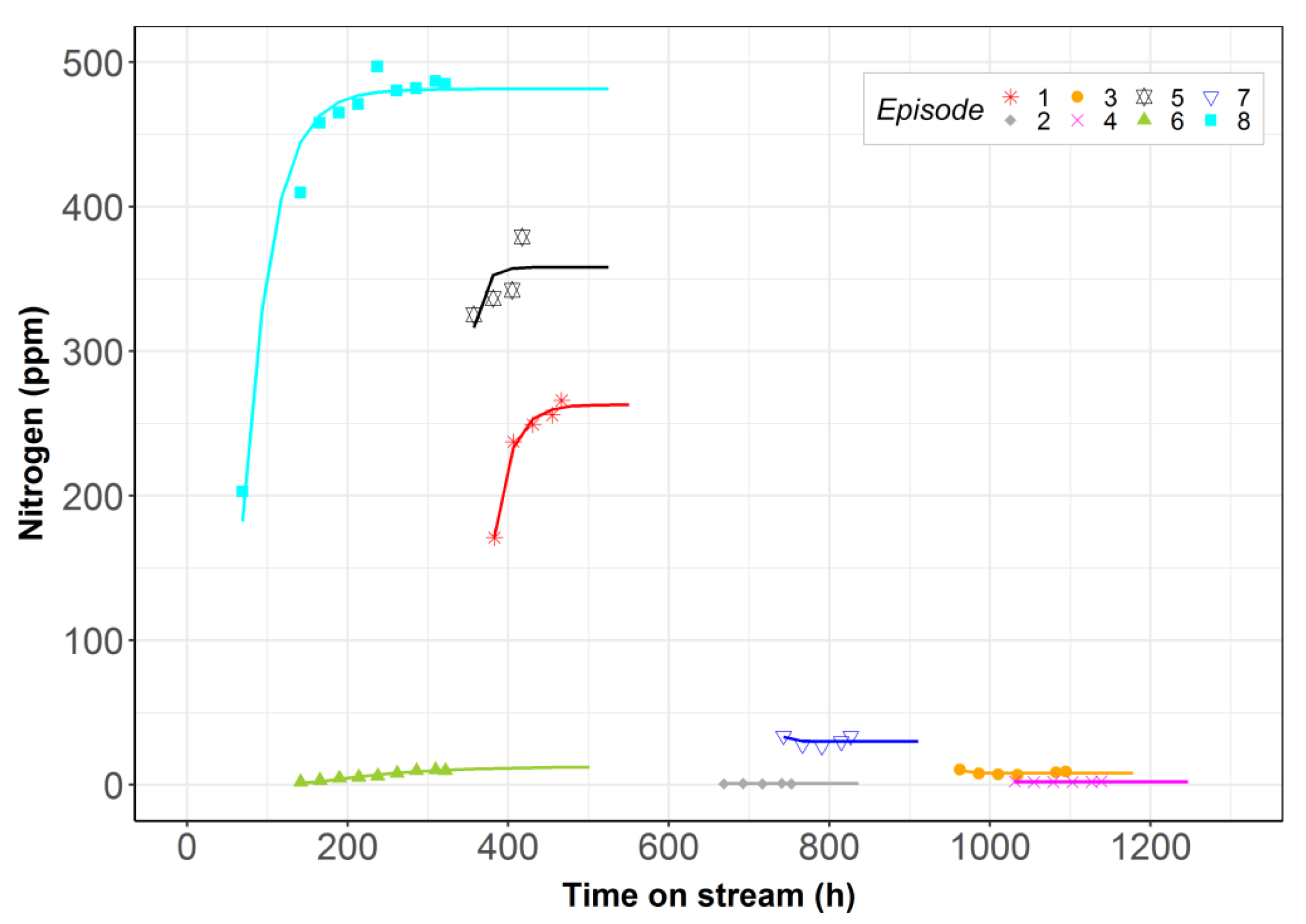
Figure 2 also shows that a good model fitting can be obtained from eight episodes onwards, selected by the Kennard–Stone algorithm. The prediction accuracy using the parameter estimates obtained against the data including stabilization then converged to its lowest value. The obtained results indicate that the Kennard–Stone technique can effectively be used to determine the operating conditions for transient experiments. As Kennard–Stone is a technique based on the distance of points in the variable space, it can be applied for complex models when no initial parameter guesses are available. Figure 6 shows the liquid effluent nitrogen as a function of time on stream of these eight episodes. As can be seen, the values simulated by the model fit well the dynamic behavior of the experimental data. Table 1 completes Figure 6 with the corresponding operating conditions of each episode.
The parity plot of the 38 steady-state points is shown in Figure 7. The plot was very close to the best scenario shown in Figure 1.
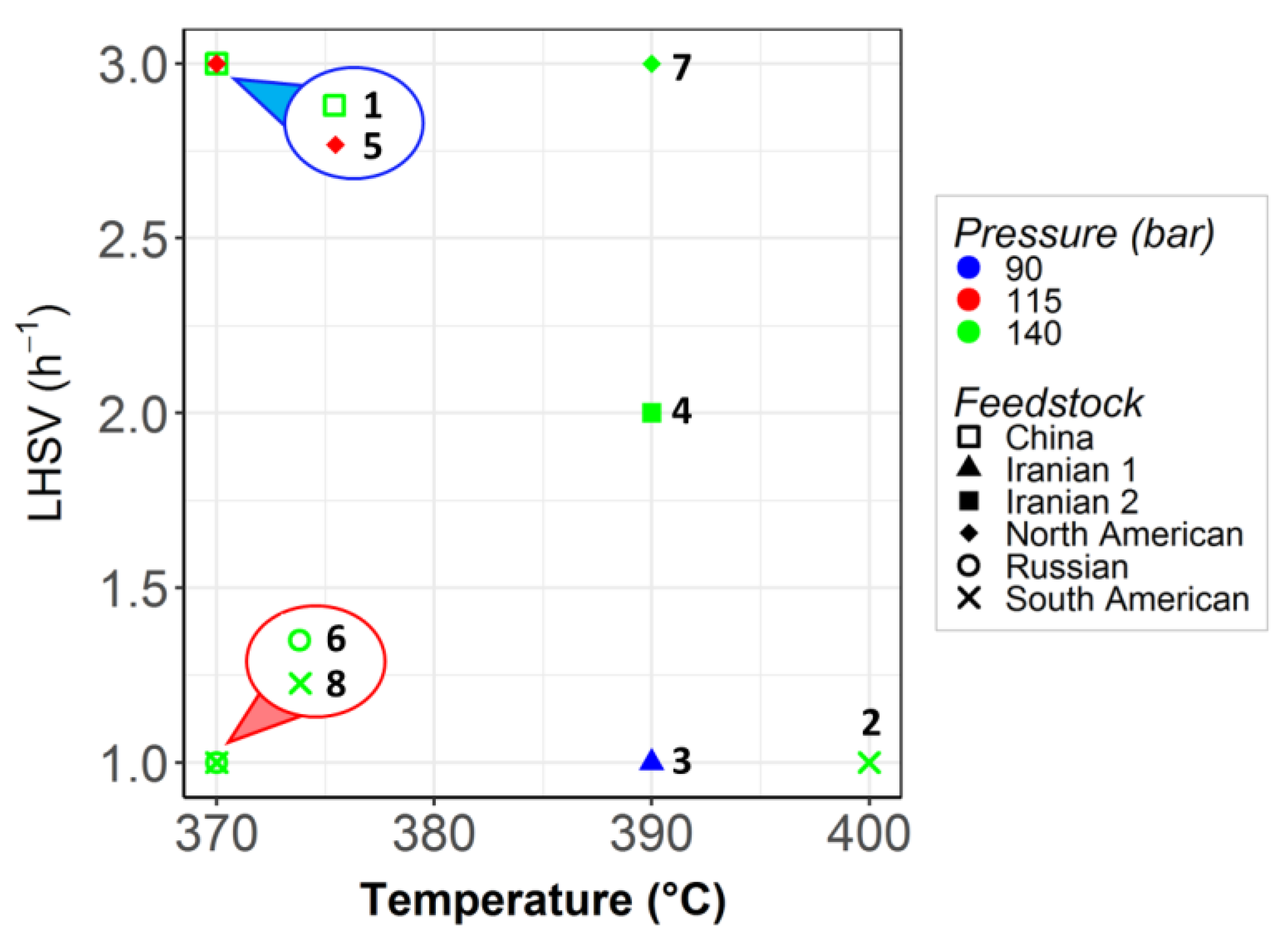
The experimental plan containing eight episodes as selected by the Kennard–Stone method is displayed in Figure 8. The selected episodes covered all the feedstocks available in the database as well as a wide range of operating conditions. The first two selected episodes were acquired at significantly different liquid hourly space velocity (LHSV), temperature, and characteristics of feedstocks. The first episode was acquired with a straight-run distillate of Chinese origin while the second one corresponded to South American heavy vacuum gas oil. Detailed characteristics of feedstocks are described in Section 3.2. As can be seen, the selected points covered the entire range of operating conditions. Regarding the feedstocks, all of them were already covered in the first six episodes. North American and South American feedstocks were then repeated in episodes 7 and 8. Regarding the LHSV and temperature, all selected episodes reached the extreme value of the investigated domain, except that episode 4 was in the middle of the region. Different values of pressure were also taken into account in the selected episodes. Episodes 1 and 2 had a similar pressure of 140 bar while it was reduced to 90 bar for episode 3. Episode 4, which had an intermediate LHSV and temperature, also had a higher pressure of 140 bar. Subsequently, episode 5 was performed at an intermediate pressure of 115 bar. The Kennard–Stone technique is more efficient than intuitive selection since it selects samples with a uniform distribution over the variable space and the selected samples can sufficiently represent the entire samples. The selected episodes could be carried out in practice within a single experimental campaign, requiring about 45~50 days (which is the maximum duration without deactivation in the pilot plant). Compared to the case of two campaigns lasting 90~100 days and 15 days of catalyst unloading/loading in-between, exploiting transient data generates a tremendous time-and-cost saving around 50% in time and cost. Furthermore, mathematically speaking, the model parameters could be identified by using only transient data at a shorter time (i.e., no need to wait for the steady state). However, the impact of changing operating conditions when the steady state has not been reached needs to be analyzed.

2.2. Model Robustness

The robustness test explained in Section 3.3.4 was carried out. The RMSE on the validation database comprising 23 episodes is illustrated in Figure 9. Blue circles and red crosses represent the steady-state model and the model including stabilization, respectively. The results indicate that the prediction accuracy when using the parameters estimated against data including stabilization was more stable and lower than when only steady-state data were used to estimate the parameters. The statistics mean (μ) and standard deviation (σ) of the distribution of MAPE and RMSE for each case are also summarized in Table 2. The mean of RMSE was 28.6 and 20.6 for the steady-state model and model including stabilization, respectively. The higher standard deviation in the “steady-state model” case reflects the more significant impact of outliers when using only steady-state data.
Accounting for stabilization was, hence, found to be more robust to outliers, as was possible with the nitrogen measurements. It can be explained by the fact that by employing the transient data, the model was fitted to an entire episode, which is an ordered series of points and not a random one. The points in an episode well represented the episode so that the impact of an outlier on one of them was less pronounced on model fitting. This demonstration confirms the interest of exploiting transient data.

3. Materials and Methods

3.1. Pilot Plant

The experimental data were obtained using a hydrotreating pilot plant located at IFP Energies Nouvelles, Solaize, France. The latter comprises four parallel fixed bed reactors, operated in down-flow mode. The catalyst volume of each reactor amounts to 50 cm3. Temperature is controlled along the reactor to ensure isothermal operation. During the experiment, effluent properties such as nitrogen content, density, and refractive index were determined every 24 hours. The steady state is considered to be established when these effluent properties are stabilized. After this, the operating conditions were switched to those corresponding with the next experimental measurement. It is worth noting that transient data have not been acquired for the purpose of using them for kinetic modeling at first, but are part of the evolution toward steady state during catalyst evaluation.

3.2. Operating Conditions and Feedstocks

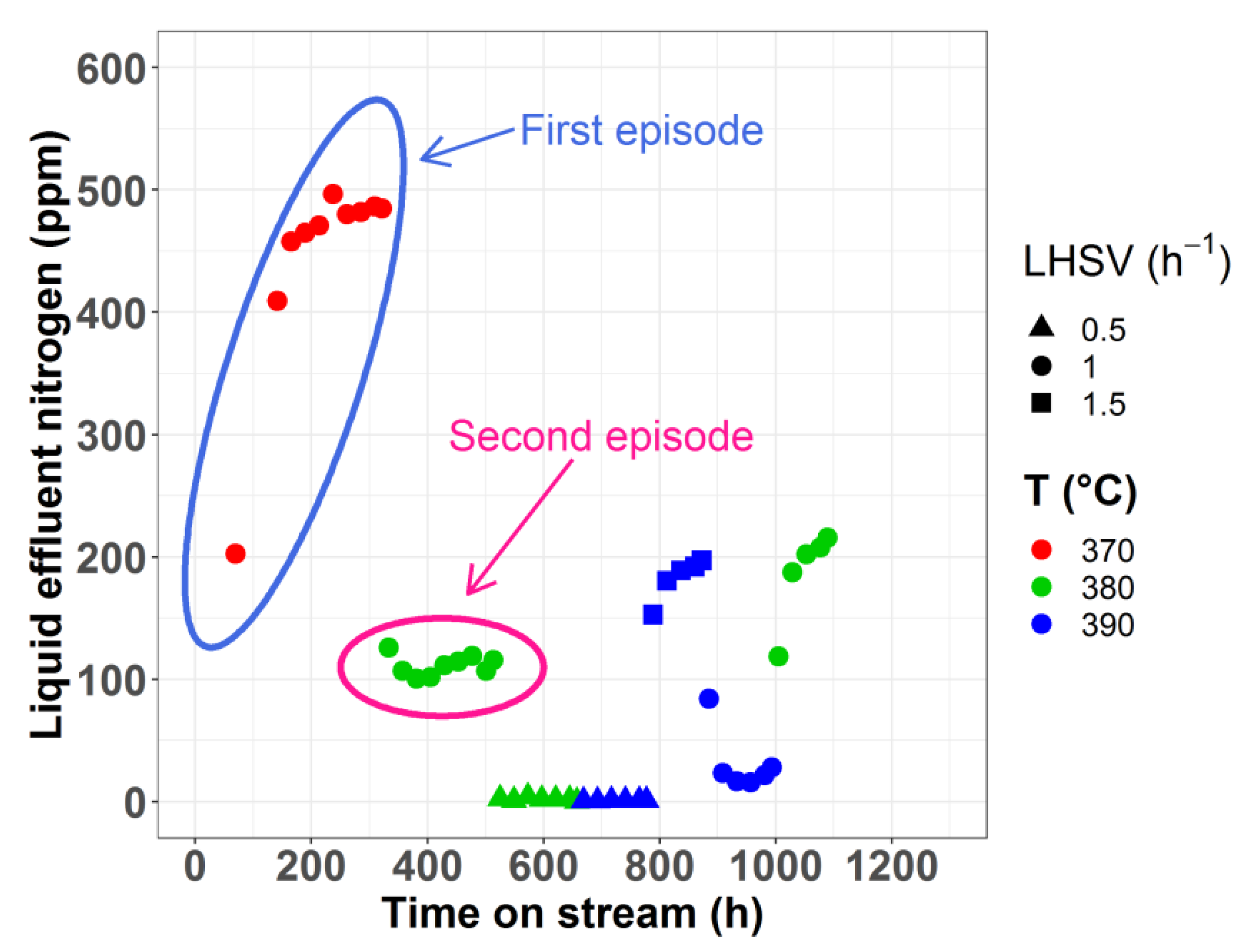
Experimental points were measured in terms of nitrogen content in the liquid effluent over time on stream. For one set of operating conditions, the series of consecutive experimental points obtained during transient regime until reaching the steady-state is denoted as an ‘episode’ [27]. In other words, consecutive experimental data points at the same operating conditions were recorded as one episode. Figure 10 shows an example of one experimental test comprising seven episodes totaling 42 data points acquired in about 45 days. The first episode corresponded to the start of the test at specific operating conditions, while later episodes were initiated by a change in operating conditions such as LHSV or temperature. Note that LHSV represents the ratio of liquid volumetric flowrate and the catalyst volume in the reactor, which is the inverse of the space time.
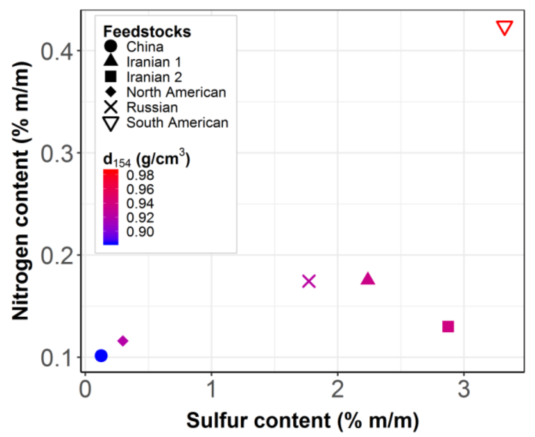
The entire database employed in this work covered 38 episodes with a total of 233 data points (i.e., 38 steady-state points and 195 transient points. The latter represents 84% of the total number of points in the database. Data covered different feedstocks over a single industrial hydrotreating catalyst within a wide range of operating conditions: LHSV from 1 to 3 h−1, temperature between 370 and 400 °C, and total pressure between 90 and 140 bar. The latter were similar to industrially employed hydrocracker conditions. Note that the low LHSV of 0.5 h−1 led to a very low level of organic nitrogen in the total liquid product. The latter were considered less reliable for model construction and parameter determination. Nevertheless, the model constructed based on the data excluding the measurements at LHSV 0.5 h−1 could properly reproduce the latter data. Six feedstocks with diverse characteristics were covered: one Russian blend of cracked feedstock, one South American heavy vacuum gas oil, and four straight-run distillates of North American, Iranian (2), and Chinese origin. The Russian and Iranian feedstocks were low in specific gravity and nitrogen content, but were high in sulfur content while that of the South American origin was heavier and contained more nitrogen and sulfur. The feedstocks of North American and Chinese origin were lighter and contained less nitrogen as well as sulfur. These feedstocks provide good diversity in the database to construct a robust model that can be used for a variety of different feedstocks. The characteristics of feed and the operating conditions are respectively shown in Figure 11.

3.3. Modeling

3.3.1. Kinetic Model

Hydrodenitrogenation was selected as a study case in this work since it is a crucial reaction in hydrotreating to remove nitrogen from hydrocarbons, avoiding hydrocracking catalyst poisoning by organic nitrogen. Hydrotreatment reaction was previously described using a continuous lumping approach by our team [7]. The pseudo kinetic model for hydrodenitrogenation was used for the purpose of simplicity. The “steady-state hydrodenitrogenation kinetic model” is given in Equation (1). It contains 11 parameters (i.e., k0, E, m, n, a, b, A0, C0, u, tt, and v). The temperature dependence of the rate coefficient is expressed via a reparametrized Arrhenius equation in which k0 is the reference rate coefficient at T0 and E is the activation energy of the reaction. Other parameters account for the actual oil composition as well as H2 partial pressure (see also the nomenclature in the Appendix A). The numerator in the equation represents the reaction kinetics while the denominator accounts for composition effects. The rest term performs the thermodynamic limit.
d C N d t = k 0 exp ( E R ( 1 T 1 T 0 ) ) ( p p H 2 p p H 2 , r e f ) m C N n ( 1 + A 0 R e s 0 ) ( 1 + C 0 C N , 0 C S , 0 ) × ( 1 u ( p p H 2 p p H 2 , r e f ) a exp ( b R ( 1 T 1 T 0 ) ) ( T M P T M P r e f ) v C N t t )
The main idea is to include the stabilization effects as a function of time on stream in the rate expression presented in Equation (1). During the transient stabilization phase, the catalyst undergoes modifications that are accounted for according to a first-order response [27]. Both the total number of sites as well as their ‘activity’ are assumed to evolve in a first-order manner. As a result, the reference rate coefficient k0 is multiplied by a first-order transfer function f and the activation energy E and b are multiplied by another first-order transfer function g. By including these transfer functions in the model, Equation (2) is obtained as below:
d C N d t = f × k 0 e x p ( E × g R ( 1 T 1 T 0 ) ) ( p p H 2 p p H 2 , r e f ) m C N n ( 1 + A 0 R e s 0 ) ( 1 + C 0 C N , 0 C S , 0 ) × ( 1 u ( p p H 2 p p H 2 , r e f ) a e x p ( b × g R ( 1 T 1 T 0 ) ) ( T M P T M P r e f ) v C N t t )
In our previous work [27], it was found that the stabilization due to hydrodynamics was significantly faster than the real observed stabilization. The first-order response found for the latter was not due to the macroscopic physical variables, but mainly driven by chemical phenomena. The stabilization behavior can be mathematically described as the response of the process to a slowly varying operating condition (e.g., instead of the state of the catalyst), which is denoted as the apparent operating condition. LHSV and temperature were changed in the experimental test. The function f is then defined as the evolution of LHSV versus time on stream when changing LHSV from episode (i − 1) to episode i. The function f is shown in Equation (3) where LHSVapp is the apparent LHSV.
f i   ( T O S ) = L H S V i L H S V a p p = L H S V i L H S V i 1 + ( L H S V i L H S V i 1 ) × ( 1 e x p ( T O S T O S i n i t _ i τ i ) )
The same structure is used for transfer function g, see Equation (4). It is built under a hypothesis of the temperature evolution during stabilization. Tapp in Equation (4) is the apparent temperature that evolves from the temperature of episode (i − 1) to the temperature of episode i.
g i   ( T O S ) = T i T a p p = T i T i 1 + ( T i T i 1 ) × ( 1 e x p ( T O S T O S i n i t _ i τ i ) )
Here, τ i appearing in Equations (3) and (4) is the parameter representing the characteristic time of episode i, called ‘transient parameter’. For each episode, only one τ is attributed to the variation of LHSVapp and Tapp. Upon a feedstock change, the apparent feedstock composition representing the slowly varying change from the previous feedstock to the new one (i.e., organic nitrogen, sulfur, and resin content) is employed in the kinetic model.
By substituting Equations (3) and (4) in Equation (2), the ‘model including stabilization’, as shown in Equation (5) is obtained.
d C N d t = L H S V L H S V a p p k 0 e x p ( E R T T a p p ( 1 T 1 T 0 ) ) ( p p H 2 p p H 2 , r e f ) m C N n ( 1 + A 0 R e s 0 ) ( 1 + C 0 C N ,   0 C S ,   0 )          × ( 1 u ( p p H 2 p p H 2 , r e f ) a e x p ( b R T T a p p ( 1 T 1 T 0 ) ) ( T M P T M P r e f ) v C N t t )
The model including the stabilization function contains the 11 kinetic parameters (identical to steady-state kinetic model) and a number of transient parameters τi corresponding to the number of episodes in the calibration database. The notation ‘kinetic parameter’ was used to distinguish these 11 parameters in the steady-state kinetic model from transient parameters τi in the stabilization function. It is evident from the above equations that when the time on stream is sufficient to reach the steady state f and g converges to 1. The model including stabilization converged toward the steady-state kinetic model.

3.3.2. Parameter Estimation

Transient and kinetic parameters were determined using a calibration dataset including transient and steady-state points by minimizing the weighted least squares. In this study, the model was assumed to be correct and there was no error for the input variables. The output measurements were carried out independently and the experimental errors were assumed to be normally distributed with a mean of 0 and a constant standard deviation. As the steady-state points are supposed to contain more reliable information for the parameter estimation, it is supposed that the closer the point is to the steady state, the higher the weight that can be attributed to it. The weight of the steady-state points was set at 1. Equation (6) is used to calculate the weight of the transient data points:
w i j = T O S i j T O S i n i t _ i T O S i _ f i n a l T O S i n i t _ i  
where wij is the weight of point j in episode I; TOSij is the time on stream of point j in episode i (h); TOSi_final is time on stream of the last point in episode i where the steady state is reached (h); and TOSinit_i is the beginning of episode i (h).
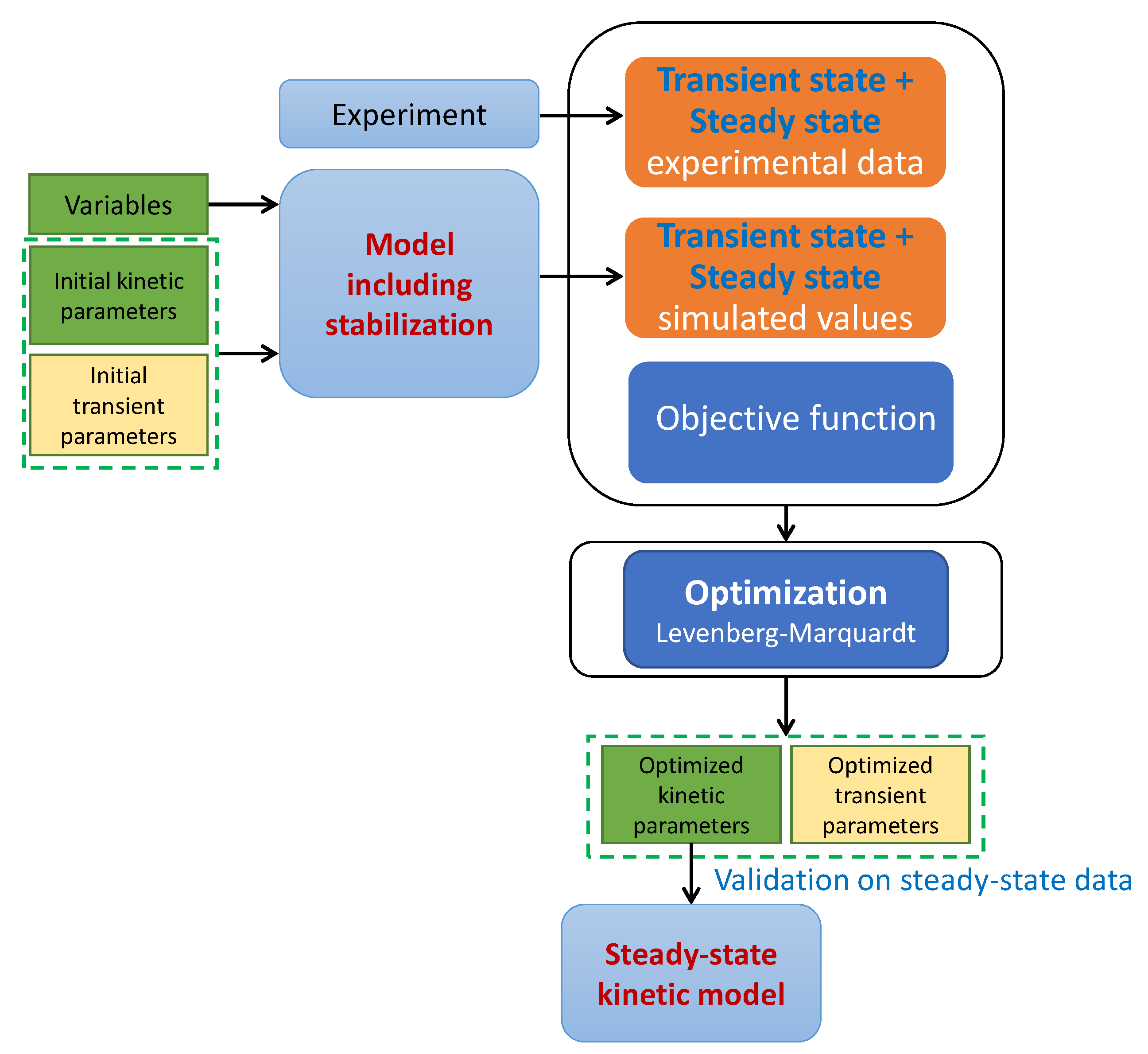
Figure 12 shows the parameter estimation algorithm for the model including stabilization. The model simulates the output variable by using the transient and kinetic parameters as well as the input variables. The calculated response value was compared with the experimentally observed one via an objective function, which is the sum of weighted squared relative errors. A Levenberg–Marquardt algorithm [29,30] was used to determine the minimum of this objective function. As the problem is nonlinear, the optimization may yield a local minimum (i.e., it does not guarantee the identification of the global minimum). Therefore, we needed to repeat the optimization a number of times using randomly selected initial parameters. Only the optimal parameters corresponding to a minimum value of objective function were retained. The optimal kinetic parameters were then validated by using a validation database at the steady-state condition. Whether stabilization was accounted for or not, the parameter estimation procedure was identical, except that the transient parameters are irrelevant when considering the steady-state data only. Hence, the data at steady-state condition can be employed to calibrate the steady-state model while the transient as well as steady-state data can be included in the calibration database to tune the model including stabilization. The technique to obtain the calibration and validation database is described in Section 3.3.3.

3.3.3. Comparison Strategy

The entire database was first split into the calibration and validation database. The calibration database was used to estimate the parameters in the models as discussed above. The estimated parameters were then tested on the validation dataset. Kinetic parameters estimated using steady-state data only or steady-state and transient data were compared several times via different calibration and validation databases. Data splitting can be carried out via some experimental design techniques. The techniques adopted in the present work where the Kennard–Stone algorithm [31] and D-optimal design [32,33,34].
The Kennard–Stone technique intends to select the best representative subset from all the candidates available based on their Euclidean distance. The Euclidean distance between two n-components vectors Xp and Xq is shown in Equation (7) [35]:
E D ( X p , X q ) = E D ( X q , X p ) = j = 1 n ( x j ,   p x j ,   q ) 2
where n represents the number of components in vector X; xj,p and xj,q are the jth component of vector Xp and Xq, respectively. The method assumes that Xp and Xq are dissimilar when the distance between them is high and similar when the distance is low. The Kennard–Stone algorithm is a step-by-step procedure. First, the two candidate points with the largest Euclidean distance are selected. After that, the candidate point that displays the greatest distance with respect to the selected points is added to the list. The distance between the candidate point and the selected points is the distance from the candidate point to its closest selected point. This step is repeated until reaching the required number of samples.
D-optimality represents an alternative technique within the possibilities for model-based experimental design. It is based on the optimization of the eigenvalues of the information matrix (i.e., the inverse of the variance-covariance matrix). The parameter estimates and corresponding joint confidence interval form an ellipsoid that is characterized by the eigenvalues of this matrix. The aim of the model-based experimental design is to reduce the eigenvalues, which correspondingly reduces the volume of the joint confidence interval of the parameter estimates. Different criteria can be considered:
  • D-criterion: maximize the determinant of the information matrix, which means minimizing the volume of the ellipsoid
  • A-criterion: minimize the sum of eigenvalues that correspond to the trace of the variance-covariance matrix
  • E-criterion: minimize the largest eigenvalues that minimizes the size of the larger axis of the confidence region, also denoted as the shape criterion.
Since D-criterion was found to be the most widely used criterion [36], we decided to employ D-optimal design to split the database. More dedicated articles can be found in the literature for the readers interested in D-optimal design [32,36,37].
Applying this to our problem, each episode is considered as a candidate and, hence, the entire database corresponded to 38 candidates. Regarding the Kennard–Stone method, the variables established vector X comprised the feed properties (organic nitrogen, sulfur, resin content, specific gravity) and the operating conditions (LHSV, temperature, total pressure). Different calibration databases were constructed with the number of episodes running from two (the minimum selected candidates) to 20 episodes. D-optimal design was applied using the steady-state model. As D-optimal design is a model-based technique, the minimum number of selected episodes from D-optimal was 12 (i.e., number of parameters + 1) [36]. The selected number of episodes for the calibration dataset varied from 12 to 20 in the case of D-optimality. The corresponding validation databases for both techniques were the leftover steady-state points of non-selected episodes.
At each defined number of selected episodes, the calibration database was employed to estimate the parameters (transient and steady-state points for the model including stabilization and steady-state points for the hydrodenitrogenation kinetics model only). After that, the optimal kinetic parameters were tested on the validation database. The effect of the size of the calibration database was also investigated via the comparison on different calibration databases. To be able to compare the prediction accuracy of both modeling strategies, the quality performance was calculated based on 38 steady-state points of 38 episodes. The used metrics of the MAPE and RMSE formula are given in Equations (8) and (9). As liquid product nitrogen in the experimental data varies across a wide range of values (0.6–500 ppm), it is preferable to simultaneously analyze MAPE and RMSE to compare the prediction accuracy. The results were also compared with the best scenario when all 38 steady-state points were used to calibrate the steady-state model.
M A P E = 100 % n i = 1 n | y i s i m y i e x p y i e x p |  
R M S E = 1 n i = 1 n ( y i s i m y i e x p ) 2  
Parameter uncertainties were estimated from the covariance matrix. The 95% confidence interval of parameter estimate θi can be calculated using Equation (10), where seθi is the standard error of parameter θi approximated as the square root of the diagonal element of the covariance matrix and t(0.95, df) is the value of the Student t-distribution at 95% confidence level for df degrees of freedom. The covariance matrix was estimated via the inverse of the Hessian matrix (i.e., the negative second-order partial derivatives of the objective function).
C I θ i = θ i ± s e θ i × t ( 0.95 ,     d f )
The model was coded in Fortran 2008. The ODE was solved using LSODE solver from the SLATEC mathematical library [38]. Parameter estimation was carried out using the DN2FB solver from the PORT library [39]. An executable file (.exe) based on the code was created to ease the implementation. The file was then called from R software version 3.6.1, which is a free software environment supported by the R Foundation for Statistical Computing. In R, there are several packages dedicated to data analysis and statistics. The statistical analysis was carried out using the ’base’ package. Figures were produced using ‘ggplot’ in the ‘ggplot2’ package. Regarding the experimental design algorithm, Kennard–Stone and D-optimal were undertaken by using the ‘kenStone’ function in the ‘prospectr’ package and ‘optFederov’ function in the ‘AlgDesign’ package, respectively.

3.3.4. Robustness

During experimentation, atypical observations, also denoted as ‘outliers’, may occur. In this work, robustness is defined as the stability of the model prediction accuracy in the presence of outliers. An outlier in the calibration database might have an impact on the parameter estimation in the case of the steady-state model since the outlier point is fitted to estimate the kinetic parameter. As the regression using the transient measurements uses more data points than the one based on the steady-state measurements, it can be expected to be more robust to outliers. In order to test the robustness of the kinetic model using transient points, the whole database was split into a calibration database containing 15 episodes selected by the Kennard–Stone algorithm (15 steady-state points + 89 transient points, which totaled 104 points) and a validation database with 23 steady-state points from the remaining episodes. Outliers can occur in the transient as well as in the steady-state measurements. A total of 20% of the steady-state points and 20% of transient and steady-state points were randomly selected for the steady-state model and the model including stabilization, respectively. The noise was artificially added to the selected points in the calibration database by varying them randomly in a severe manner at either +25% or −25%. Organic nitrogen measured using a chemiluminescence detector [40] has an uncertainty around ± 10%. The percentage of 25% aims to imitate an extreme outlier case. The scenario of selecting points is summarized in Table 3. Since the points to be modified were randomly selected, the procedure was repeated 300 times. The steady-state model and the model including stabilization were calibrated via the ‘noisy’ calibration dataset. Estimated kinetic parameters were then tested on the validation database so that the metrics MAPE and RMSE on the validation set (23 steady-state points) could be estimated.

4. Conclusions

The long stabilization in hydroprocessing has been addressed as one of the major challenges in experimental data collection for kinetic modeling. A methodology exploiting transient data to determine the parameters in a kinetic model for hydrodenitrogenation has been devised by employing a model considering the stabilization as a function of time on stream. Stabilization is considered to follow a first-order behavior characterized by parameter τ, specifically accounting for the transient phenomena.
The results demonstrate that accounting for stabilization results in a similar prediction accuracy as when relying on steady-state data only. The parameter values can already be determined from a lower number of episodes and, hence, steady-state points, thanks to the explicit use of transient data contained in these episodes. It significantly reduces, i.e., up to halving, the duration of experimental work for kinetic modeling. Transient data also help to reduce the impact of outliers on the model quality, which makes the model including stabilization more robust than the steady-state one. By combining with an experimental design technique such as the Kennard–Stone algorithm, transient data can accelerate parameter identification. The Kennard–Stone method has been found to provide a representative experimental plan for the transient experiments.
Catalyst research and development work aims to improve the efficiency and performance and to reduce the cost as well as to reduce the development time, in order to respond expeditiously to market demand. Exploiting transient data is a very promising approach to save enormous time and cost regarding experimental work for kinetic model construction.

Author Contributions

Conceptualization, B.C., D.G., I.G. and J.W.T.; Methodology, B.C., D.G., and N.-Y.-P.C.; Software, N.-Y.-P.C.; Validation, B.C., D.G., I.G., and J.W.T.; Formal analysis, N.-Y.-P.C.; Investigation, N.-Y.-P.C.; Resources, I.G.; Data curation, N.-Y.-P.C.; Writing—original draft preparation, N.-Y.-P.C.; Writing—review and editing, all authors; Visualization, N.-Y.-P.C.; Supervision, B.C., D.G., I.G., and J.W.T.; Project administration, B.C. and J.W.T.; Funding acquisition, B.C. All authors have read and agreed to the published version of the manuscript.

Funding

This research received no external funding.

Conflicts of Interest

The authors declare no conflicts of interest.

Appendix A

Nomenclature
aOrder associated with hydrogen partial pressure in thermodynamic term-
A0Resin adsorption coefficient-
bParameter in thermodynamic term-
C0Coefficient of the ratio nitrogen/sulfur in feedstock-
CNOrganic nitrogen concentration in liquid output streamppm m/m
CN,0Organic nitrogen concentration in feedppm m/m
CS,0Organic sulfur concentration in feed% m/m
EActivation energyJ.mol−1
fiTransfer function f of episode i-
giTransfer function g of episode i-
k0Rate constant at T0-
LHSVLiquid hourly space velocityh−1
LHSVappApparent liquid hourly space velocity of episode ih−1
LHSViLiquid hourly space velocity of episode ih−1
LHSVi−1Liquid hourly space velocity of episode i − 1h−1
mOrder of ppH2-
nOrder of concentration of organic nitrogen-
ppH2Hydrogen partial pressure bar
ppH2,refReference H2 partial pressurebar
RIdeal gas constantJ·mol−1·K−1
res0Feed resin% m/m
tResidence timeh
TReactor temperatureK
T0Reference temperatureK
TappApparent temperature of episode iK
TiTemperature of episode iK
Ti−1Temperature of episode i − 1K
TMPWeighted average temperature of simulated distillation by gas chromatography of feed°C
TMPrefReference weighted average temperature of simulated distillation by gas chromatography°C
TOSTime on streamh
TOSi−1Time on stream of the last point of episode i − 1h
TOSinit_iTime on stream when the episode i startsh
ttOrder of concentration of organic nitrogen in thermodynamic term-
ufactor in thermodynamic term-
vOrder associated with the heaviness of feed-
τiStabilization time at episode ih

References

  1. Speight, J.G. Hydrocracking. In The Refinery of the Future, 1st ed.; Speight, J.G., Ed.; Gulf Professional: London, UK, 2011; pp. 275–313. ISBN 9780815520412. [Google Scholar]
  2. Bricker, M.; Thakkar, V.; Petri, J. Hydrocracking in Petroleum Processing. In Handbook of Petroleum Processing; Treese, S.A., Pujadó, P.R., Jones, D.S.J., Eds.; Springer: Cham, Switzerland, 2015; pp. 317–359. ISBN 978-3-319-14528-0. [Google Scholar]
  3. Stratas Advisors. 13 Countries Move Up in Top 100 Ranking on Diesel Sulfur Limits | Stratas Advisors. Available online: https://stratasadvisors.com/Insights/2019/022819-Top-100-Diesel-Sulfur-Ranking (accessed on 15 January 2020).
  4. IMO. Sulphur 2020—Cutting Sulphur Oxide Emissions. Available online: http://www.imo.org/en/mediacentre/hottopics/pages/sulphur-2020.aspx (accessed on 15 January 2020).
  5. Ancheyta, J.; Sánchez, S.; Rodríguez, M.A. Kinetic modeling of hydrocracking of heavy oil fractions: A review. Catal. Today 2005, 109, 76–92. [Google Scholar] [CrossRef]
  6. Jarullah, A.T.; Mujtaba, I.M.; Wood, A.S. Kinetic model development and simulation of simultaneous hydrodenitrogenation and hydrodemetallization of crude oil in trickle bed reactor. Fuel 2011, 90, 2165–2181. [Google Scholar] [CrossRef]
  7. Becker, P.J.; Celse, B.; Guillaume, D.; Dulot, H.; Costa, V. Hydrotreatment modeling for a variety of VGO feedstocks: A continuous lumping approach. Fuel 2015, 139, 133–143. [Google Scholar] [CrossRef]
  8. Esmaeel, S.A.; Gheni, S.A.; Jarullah, A.T. 5-Lumps kinetic modeling, simulation and optimization for hydrotreating of atmospheric crude oil residue. Appl. Petrochem. Res. 2016, 6, 117–133. [Google Scholar] [CrossRef] [Green Version]
  9. Lababidi, H.M.S.; AlHumaidan, F.S. Modeling the hydrocracking kinetics of atmospheric residue in hydrotreating processes by the continuous lumping approach. Energy Fuels 2011, 25, 1939–1949. [Google Scholar] [CrossRef]
  10. Tang, X.; Li, S.; Yue, C.; He, J.; Hou, J. Lumping kinetics of hydrodesulfurization and hydrodenitrogenation of the middle distillate from chinese shale oil. Oil Shale 2013, 30, 517. [Google Scholar] [CrossRef] [Green Version]
  11. Bonnardot, J. Kinetic Modelling of Hydro-Treatment Reactions by Study of Different Chemical Groups. Ph.D. Thesis, Claude Bernard University, Lyon, France, 1998. [Google Scholar]
  12. López García, C.; Hudebine, D.; Schweitzer, J.-M.; Verstraete, J.J.; Ferré, D. In-depth modeling of gas oil hydrotreating: From feedstock reconstruction to reactor stability analysis. Catal. Today 2010, 150, 279–299. [Google Scholar] [CrossRef]
  13. Oyekunle, L.O.; Edafe, O.A. Kinetic modeling of hydrodenitrogenation of pyridine. Pet. Sci. Technol. 2009, 27, 557–567. [Google Scholar] [CrossRef]
  14. Raghuveer, C.S.; Thybaut, J.W.; Marin, G.B. Pyridine hydrodenitrogenation kinetics over a sulphided NiMo/γ-Al2O3 catalyst. Fuel 2016, 171, 253–262. [Google Scholar] [CrossRef]
  15. Nguyen, M.-T.; Tayakout-Fayolle, M.; Pirngruber, G.D.; Chainet, F.; Geantet, C. Kinetic modeling of quinoline hydrodenitrogenation over a NiMo(P)/Al2O3 catalyst in a batch reactor. Ind. Eng. Chem. Res. 2015, 54, 9278–9288. [Google Scholar] [CrossRef]
  16. Nguyen, M.-T.; Pirngruber, G.D.; Chainet, F.; Tayakout-Fayolle, M.; Geantet, C. Indole hydrodenitrogenation over alumina and silica—Alumina-supported sulfide catalysts—Comparison with quinoline. Ind. Eng. Chem. Res. 2017, 56, 11088–11099. [Google Scholar] [CrossRef]
  17. Doukeh, R.; Bombos, M.; Trifoi, A.; Mihai, O.; Popovici, D.; Bolocan, I.; Bombos, D. Kinetics of thiophene hydrodesulfurization over a supported Mo-Co-Ni catalyst. Comptes Rendus Chimie 2018, 21, 277–287. [Google Scholar] [CrossRef]
  18. Charon-Revellin, N.; Dulot, H.; López-García, C.; Jose, J. Kinetic modeling of vacuum gas oil hydrotreatment using a molecular reconstruction approach. Oil Gas Sci. Technol. Rev. IFP Energies Nouv. 2011, 66, 479–490. [Google Scholar] [CrossRef] [Green Version]
  19. Schweitzer, J.-M.; Galtier, P.; Schweich, D. A single events kinetic model for the hydrocracking of paraffins in a three-phase reactor. Chem. Eng. Sci. 1999, 54, 2441–2452. [Google Scholar] [CrossRef]
  20. Elkamel, A.; Al-Ajmi, A.; Fahim, M. Modeling the hydrocracking process using artificial neural networks. Pet. Sci. Technol. 1999, 17, 931–954. [Google Scholar] [CrossRef]
  21. Bahmani, M.; Sharifi, K.; Shirvani, M. Product Yields Prediction of Tehran Refinery Hydrocracking Unit Using Artificial Neural Networks. Iran. J. Chem. Eng. 2010, 7, 50–63. [Google Scholar]
  22. Sadighi, S.; Reza Zahedi, G. Comparison of kinetic-based and artificial neural network modeling methods for a pilot scale vacuum gas oil hydrocracking reactor. Bull. Chem. React. Eng. Catal. 2013, 8. [Google Scholar] [CrossRef] [Green Version]
  23. Sadighi, S.; Mohaddecy, S.R.S. Evaluating the ability of R for modeling a commercial scale VGO hydrocracking plant using Artificial Neural Network (ANN). Pet. Coal 2018, 60, 358–364. [Google Scholar]
  24. de Oliveira, L.P.; Hudebine, D.; Guillaume, D.; Verstraete, J.J.; Joly, J.F. A Review of Kinetic Modeling Methodologies for Complex Processes. Oil Gas Sci. Technol. Rev. IFP Energ. Nouv. 2016, 71, 45. [Google Scholar] [CrossRef] [Green Version]
  25. Yang, S.H.; Satterfield, C.N. Some effects of sulfiding of a NiMoAl2O3 catalyst on its activity for hydrodenitrogenation of quinoline. J. Catal. 1983, 81, 168–178. [Google Scholar] [CrossRef]
  26. Sau, M.; Basak, K.; Manna, U.; Santra, M.; Verma, R.P. Effects of organic nitrogen compounds on hydrotreating and hydrocracking reactions. Catal. Today 2005, 109, 112–119. [Google Scholar] [CrossRef]
  27. Cao, N.-Y.-P.; Celse, B.; Guillaume, D.; Guibard, I.; Thybaut, J.W. Stabilization time modeling for hydroprocessing: Identification of the dominant factors. Chem. Eng. Sci. 2020, 213. [Google Scholar] [CrossRef]
  28. Waldron, C.; Pankajakshan, A.; Quaglio, M.; Cao, E.; Galvanin, F.; Gavriilidis, A. An autonomous microreactor platform for the rapid identification of kinetic models. React. Chem. Eng. 2019, 47, 2331. [Google Scholar] [CrossRef] [Green Version]
  29. Marquardt, D.W. An algorithm for least-squares estimation of nonlinear parameters. J. Soc. Indust. Appl. Math 1963, 11, 431–441. [Google Scholar] [CrossRef]
  30. More, J.J. The Levenberg-Marquardt Algorithm: Implementation and Theory; Springer: Berlin/Heidelberg, Germany, 1978; ISBN 978-3-540-35972-2. [Google Scholar]
  31. Kennard, R.W.; Stone, L.A. Computer aided design of experiments. Technometrics 1969, 11, 137–148. [Google Scholar] [CrossRef]
  32. Atkinson, A.C. Beyond response surfaces: Recent developments in optimum experimental design. Chemom. Intell. Lab. Syst. 1995, 28, 35–47. [Google Scholar] [CrossRef]
  33. Aguiar, P.F.; Bourguignon, B.; Khots, M.S.; Massart, D.L.; Phan-Than-Luu, R. D-optimal designs. Chemom. Intell. Lab. Syst. 1995, 30, 199–210. [Google Scholar] [CrossRef]
  34. Pronzato, L.; Pázman, A. Design of Experiments in Nonlinear Models; Springer: New York, NY, USA, 2013. [Google Scholar]
  35. Saptoro, A.; Tadé, M.O.; Vuthaluru, H. A modified Kennard-Stone algorithm for optimal division of data for developing artificial neural Network Models. Chem. Prod. Process Modeling 2012, 7. [Google Scholar] [CrossRef]
  36. Celse, B.; Da Costa, J.J.; Costa, V. Experimental design in nonlinear case applied to hydrocracking model: How many points do we need and which ones? Int. J. Chem. Kinet. 2016, 48, 660–670. [Google Scholar] [CrossRef]
  37. Fedorov, V.V. Theory of Optimal Experiments; Academic Press: New York, NY, USA, 1972; ISBN 9780323162463. [Google Scholar]
  38. Vandevender, W.H.; Haskell, K.H. The SLATEC Mathematical Subroutine Library. Signum Newsl. 1982, 17, 16–21. [Google Scholar] [CrossRef]
  39. Fox, P.A.; Hall, A.P.; Schryer, N.L. The PORT Mathematical Subroutine Library. ACM Trans. Math. Softw. 1978, 4, 104–126. [Google Scholar] [CrossRef]
  40. Fontijn, A.; Sabadell, A.J.; Ronco, R.J. Homogeneous chemiluminescent measurement of nitric oxide with ozone. Implications for continuous selective monitoring of gaseous air pollutants. Anal. Chem. 1970, 42, 575–579. [Google Scholar] [CrossRef]
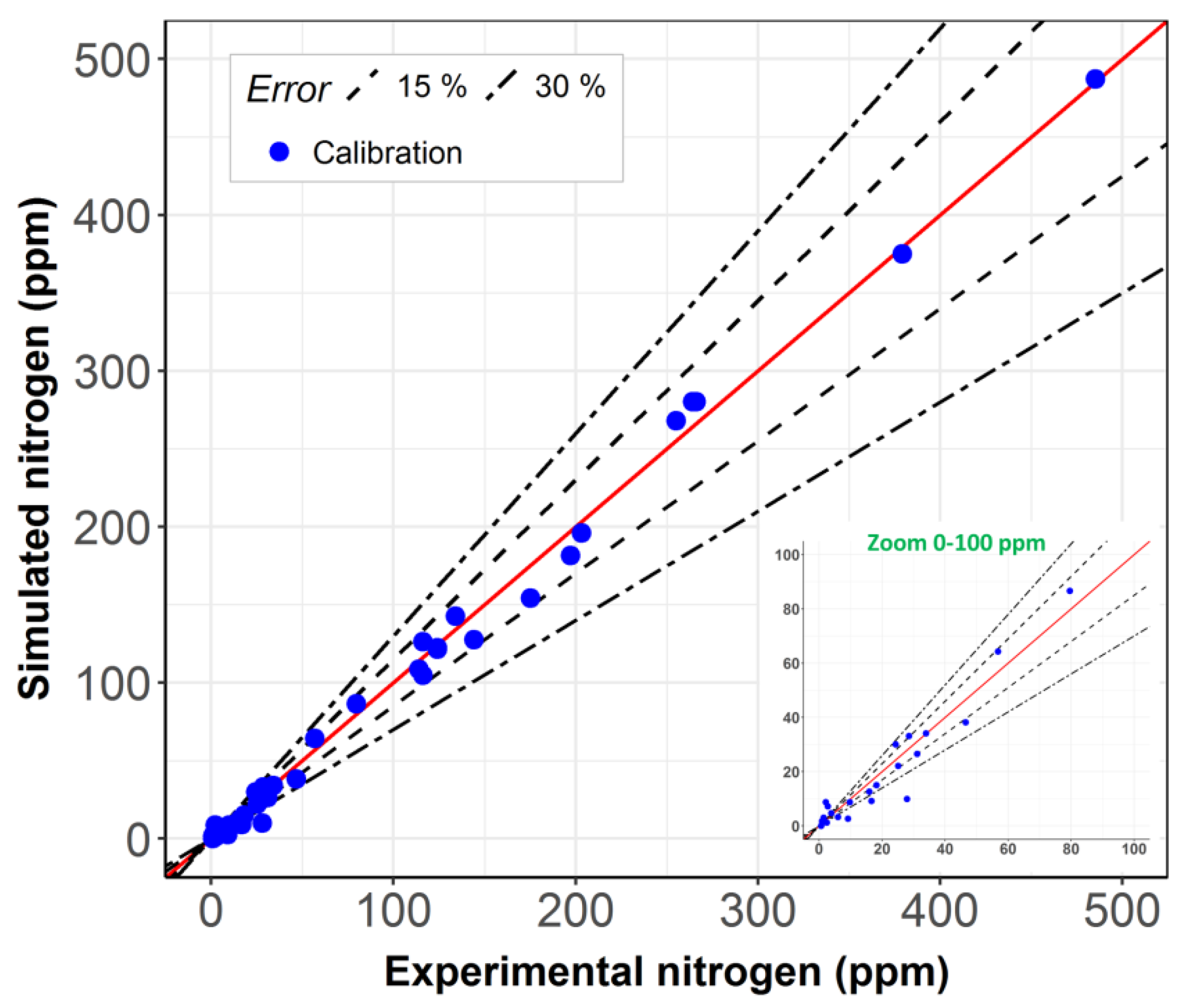
Figure 1. Parity diagram of the best scenario (calibrating steady-state model with 38 steady-state points).
Catalysts 10 00361 g001
Figure 2. Indicator mean absolute percentage error (MAPE) (a) and root mean square error (RMSE) (b) on 38 steady-state points as a function of the number of episodes in the calibration dataset (the dark green horizontal solid line represents the indicator of the best scenario).
Catalysts 10 00361 g002
Figure 3. Parity plot of steady-state model (a) (RMSE = 20.09) and model including stabilization (b) (RMSE = 14.07) for the case with the calibration database containing 14 episodes selected by the Kennard–Stone technique.
Catalysts 10 00361 g003
Figure 4. Parity plot of steady-state model (a) (RMSE = 8.23) and model including stabilization (b) (RMSE = 10.52) for the case with the calibration database containing 20 episodes selected by the D-optimal design.
Catalysts 10 00361 g004
Figure 5. Confidence interval of parameter A0 as a function of the number of episodes in the calibration database chosen by the D-optimal and Kennard–Stone algorithm.
Catalysts 10 00361 g005
Figure 6. Model calibration using eight episodes selected by the Kennard–Stone algorithm (solid line: simulated by model, points: experimental data).
Catalysts 10 00361 g006
Figure 7. Parity plot of the model with the stabilization function case with the calibration database containing eight episodes selected by the Kennard–Stone technique (MAPE = 56%, RMSE = 15).
Catalysts 10 00361 g007
Figure 8. Operating conditions of eight selected episodes (liquid hourly space velocity (LHSV) vs. temperature).
Catalysts 10 00361 g008
Figure 9. The indicator root mean square error (RMSE) on validation dataset (300 times of comparison).
Catalysts 10 00361 g009
Figure 10. Liquid effluent nitrogen as a function of time on stream (same feedstock, P = 140 bar).
Catalysts 10 00361 g010
Figure 11. Sulfur, nitrogen content, and specific gravity at 15 °C for the feedstocks in the database.
Catalysts 10 00361 g011
Figure 12. Parameter estimation framework for the “model including stabilization”.
Catalysts 10 00361 g012
Table 1. Operating conditions of eight selected episodes.
EpisodeLHSV (h−1)T (°C)P (bar)Feedstock
13370140China
21400140South American
3139090Iranian 1
42390140Iranian 2
53370115North American
61370140Russian
73390140North American
81370140South American
Table 2. Statistical results of the accuracy indicator distribution.
ModelMAPERMSE
μσμσ
Steady-state kinetic model83.943.329.112.6
Model including stabilization69.426.920.54.0
Table 3. Strategy of adding noise to the calibration database.
Steady-State Kinetic ModelModel Including Stabilization
Original calibration database15 steady-state points104 points (89 transient points + 15 steady-state points)
StrategySelect randomly and add noise to 3 steady-state points (corresponding to 20% of the original calibration database)Select randomly and add noise to 21 points, which can be transient and/or steady-state points (corresponding to 20% of the original calibration database)