Learning to Set the Reserve Price Optimally in Laboratory First Price Auctions

Abstract

We analyze choices of sellers, each setting a reserve price in a laboratory first price auction with automated equilibrium bidding. Subjects are allowed to gain experience for a fixed period of time prior to making a single payoff-relevant choice. Behavior of more experienced sellers was consistent with benchmark theory: average reserve price for these sellers was independent of the number of bidders and equaled the predicted level. Less experienced sellers however deviated from the theoretical benchmark: on average, they tended to shade reserve price below the predicted level and positively relate it to the number of bidders.

1. Introduction

For the independent private values model under benchmark conditions, auction theory predicts that the reserve price set by sellers should be independent of the number of bidders (see, e.g., Krishna 2010 [1]). Experimental studies using seller subjects and automated bidding by Greenleaf (2004) [2], investigating the English auction, and Davis, Katok and Kwasnica (2011) [3], investigating the second-price auction, however found limited support for learning or benchmark predictions. These results have been interpreted as indicating that the standard framework needs to be augmented to account for the data.

Prior studies have used the standard learning protocol, where subjects choose repeatedly for the same problem, with each choice relevant for payoff and incentives invariant across rounds, and little time or subject activity allowed in between rounds. This protocol allows the learning that takes place due to participation in payoff-relevant choice episodes and incorporation of information emerging thereof. The literature has focused on this form of learning through its use of the standard protocol. Learning can potentially also take place in between payoff-relevant choice episodes due to reconsideration of prior choice and reflection on future choice through construction of counterfactuals and hypothetical examples, which aid in providing understanding of the underlying payoff function. This form of learning has received little attention, the only exception we are aware of being Merlo and Schotter (1999) [4], which we discuss below.

In this article, we ask, for first-price auctions, whether there may exist alternate learning protocols that can enable learning and conformity of decision with prediction. This is firstly because even with the issue of conjecturing bidder behavior eliminated by informing sellers about the automated bidding rule, the problem of deciding the reserve price remains complex. Prior results suggested it may in fact be excessively complex, with little hope that optimal play can be reached, implying that auction theory may be descriptively inadequate in this regard. This conclusion has been reached under the standard protocol, i.e., when only information from payoff-relevant choice episodes is incorporated. It seems important to determine whether the failure of benchmark predictions holds for all possible learning protocols or whether there may exist protocols, perhaps allowing alternative forms of learning, which are efficacious in the sense that they can promote convergence.

Secondly, some prior evidence hints that such protocols may exist. Merlo and Schotter (1999) [4] introduced a protocol with backloaded incentives and a single payoff-relevant decision coming at the end of a learning or experience-gathering or practice phase. They argued that particular advantages of this ‘learn-before-you-earn’ (LBE) protocol, which separates the learning from the payoff-enhancement process, over the standard ‘learn-while-you-earn’ (LWE) protocol were that the former prevents a focus on the myopic stimulus-response aspect of the problem and does not penalize low-payoff outcomes during the experience phase, thus providing subjects who have not completed learning some insurance against the downside risk of experimentation, thereby permitting them to choose riskier learning strategies with the potential to yield greater eventual payoff. They analyzed this protocol in the context of a tournament game with automated partners, also a complex decision problem. They found that their LBE protocol resulted in decisions being closer to the optimal choice defined by the problem compared to an LWE protocol.

We ask as our first question therefore to what extent the benchmark receives support when seller subjects are informed about the automated bidding rule and exposed to an LBE type protocol. We vary the number of automated bidders (two or four) between subjects to address this question, the null hypothesis being that responses are invariant.

Our second question is motivated by an aspect of LBE protocols. We argue they may be quite realistic and more than just a laboratory investigative tool. In any setting that can produce learning, an individual with greater exposure to learning opportunities or experience can be expected to be capable of superior decisions or to be more skilled. Now, economic theories suggest that the structure of incentives may be differentiated by skill (see, e.g., Prendergast 1999) [5]. Together, these imply that in environments with allocative pressure such as markets where learning is possible and valuable, if experience or exposure to learning is more easily observable than underlying skill, then payoff functions or the structure of incentives may vary across individuals depending on their experience. In reality therefore, learning may often take place in environments where payoff functions are not invariant to experience. This is achieved by LBE protocols, where incentives are reserved for those who have completed learning and are maximally experienced, i.e., expected to be maximally skilled. These protocols also provide insurance to those with low exposure, who are still learning and expected to be less skilled; the combination of insurance and backloaded returns can hence be expected to provide strong incentives for learning. It is not achieved however by LWE protocols, where the incentive scheme is held constant throughout exposure, leaving the advantage of dynamically adjusting incentive schemes for learning unexploited.

The above argument implies that in settings where professionals can vary in skill level and experience, and learning is possible, forces selecting for efficiency may favor incentive schemes where more experienced individuals are more exposed to the payoff consequences of their decisions, a feature captured by LBE protocols in the limit form. The argument relies on learning being actually produced. We ask as our second question therefore whether an LBE protocol can produce learning in our decision environment, i.e., whether individuals with greater exposure to learning opportunities produce better decisions. We implement a protocol with a fixed interval of time for the learning phase rather than a fixed number of rounds. This allows individual level determination of how much information on the payoff function (number of practice choices) to acquire, and hence the choice of a potentially superior learning strategy. We vary the length of the phase (5 or 15 min) between subjects to address the question, the null hypotheses being that information acquisition and responses are invariant.

Our between-subjects experiment thus had two treatment variables, leading to a 2 × 2 factorial design. We found that while choices were invariant to the number of bidders and indistinguishable from theoretically predicted levels with a 15-min phase, they were lower than predicted ones and increasing in the number of bidders with a 5-min phase. The protocol thus appears to be capable of generating learning, with those exposed to a long phase producing decisions closer to the optimal choice defined by the problem, while those exposed to a short phase producing ones further from the optimal choice defined by the problem.

Our results indicate that experience may be a key differentiating factor in determining whether behavior can be expected to conform to the benchmark. The role of experience has been looked at in explaining deviations from benchmark bidding, in experiments with automated selling. There is considerable evidence that more experience is associated with bids deviating less from predicted levels (see the surveys of results in Kagel 1995 [6] and Kagel and Levin 2015 [7]). Our findings suggest therefore that the degree of experience can impact behavior not just on the buyer side in auction settings, but on the seller side, as well, with more experienced sellers producing decisions consistent with the benchmark. Finally, we found that while the amount of information obtained increased with the length of the phase, it was in itself unable to explain choice. These findings confirm that LBE protocols can foster learning, but suggest that any such protocol and variation in the length of its experience phase may be inducing learning strategies whose efficacy cannot be measured simply by the amount of information obtained.

Our findings indicate that benchmark theory may be capable of explaining the behavior of more experienced sellers, but could need augmentation in order to account for choices of less experienced ones. For the latter group, the fact that choices were less than predicted hints at the possibility of risk-aversion, which is compatible with such responses (see Hu, Matthews and Zou 2010 [8]). However, risk-aversion also predicts that choices should decrease in the number of bidders (Hu 2011 [9]), which is negated by our data. We therefore discard risk-aversion as a potential framework, and preference-based explanations in general, in the absence of a clear foundation as to why preference may vary with experience. Probability-weighting can provide an alternative avenue, as such models may be capable of allowing both choice to fall short of benchmark prediction and for it to increase in the number of bidders. We briefly discuss this point after presenting our results.

2. Theoretical Benchmark

A sophisticated theory has emerged for sealed bid, single unit, winner pay auctions when agents are risk-neutral and bidders are symmetric and have independent private values; see Krishna (2010) [1] for a textbook presentation. Here, we state the key results relevant for our experimental implementation, using the notation of Krishna (2010) [1].

There is one seller and N (potential) bidders. The seller has zero value for the object. Bidder i has a valuation $x_i$ for the object, which is the realization of a random variable $X_i$. These random variables $X_i,i=1,\dots ,N$ are independently and identically distributed over $[0,w]$ according to the increasing and continuously differentiable distribution function F, with corresponding density function f. The realization of $X_i$ is observed only by bidder i; all else is common knowledge.

We look at a first price auction where the seller is allowed to set a publicly known reserve price. In such an auction, bidders independently and simultaneously submit non-negative bids, and the highest bidder wins and pays the seller his/her bid in exchange for the object, provided this highest bid is no less than the reserve price. A reserve price $r\ge 0$ is a minimum level below which bids are not accepted: if all bids fall short of the reserve price, the object is not sold, and the seller earns zero revenue.

Let $Y_1$ be the highest order statistic of $N-1$ of the random variables ${\left(X_i\right)}_{i=1}^N$, and let G and g respectively be the distribution and density functions of $Y_1$. Given r, the first price auction has a unique symmetric increasing Bayesian Nash equilibrium bid function, and the equilibrium bidding strategy for any bidder with $x\ge r$ is:

$$\beta \left(x\right)=E[max(Y_1,r)|Y_1<x]=r\frac{G\left(r\right)}{G\left(x\right)}+\frac{1}{G\left(x\right)}{\int }_r^{x}yg\left(y\right)dy$$

(1)

Using (1), the seller’s expected revenue can be computed as:

$$\mathrm{\Pi }\left(r\right)=N[r\{1-F\left(r\right)\}G\left(r\right)+{\int }_r^{w}y\{1-F\left(y\right)\}g\left(y\right)dy]$$

(2)

The optimal or revenue maximizing reserve price can be determined using (2). The first order condition implies that the optimal reserve price $r^{*}$ must satisfy:

$$r^{*}=\frac{1}{\lambda \left(r^{*}\right)}$$

(3)

where $\lambda \left(x\right)=\frac{f\left(x\right)}{1-F\left(x\right)}$ is the hazard rate function associated with the distribution function F. When $\lambda (.)$ is increasing, the above condition is also sufficient, and the optimal reserve price is given by (3). A feature of the result is that the optimal reserve price is independent of the number of bidders. It is usually considered remarkable as $r^{*}$ is derived from equilibrium behavior, and bidders require data on N to arrive at equilibrium. We test this key proposition in this paper.

For our experimental implementation, we assume $w=100$ and F is uniform (for which $\lambda$ is increasing). Further, we look at two cases, one with $N=2$ and the other with $N=4$. This yields $r^{*}=50$, using (3), and, using (1),

$$\beta \left(v\right)=\left\{\begin{array}{cc}\left\{\begin{array}{cc}\frac{v^2+r^2}{2v}\hfill & ifN=2\hfill \\ \frac{3v^4+r^4}{4v^3}\hfill & ifN=4\hfill \end{array}\right.\hfill & \mathrm{for}v\ge r\hfill \\ 0\hfill & \mathrm{for}v<r\hfill \end{array}\right.$$

3. Experimental Design

The subject assumed the role of a seller selling an object facing automated bidders. Subjects were informed of this fact and also that (i) the seller had zero value for the object, (ii) each bidder had a privately known valuation, which was equally likely to be any integer in {0, .., 100}, (iii) the seller could set any integer in {0, .., 100} as a reserve price and (iv) every bidder used a particular formula that gave the bid as a function of private valuation and reserve price. They were explained the rules of the first price auction with reserve price, told how many bidders were present (two or four) and were given the relevant formula, which happened to be the risk-neutral symmetric increasing Bayesian Nash equilibrium strategy of the auction game.1

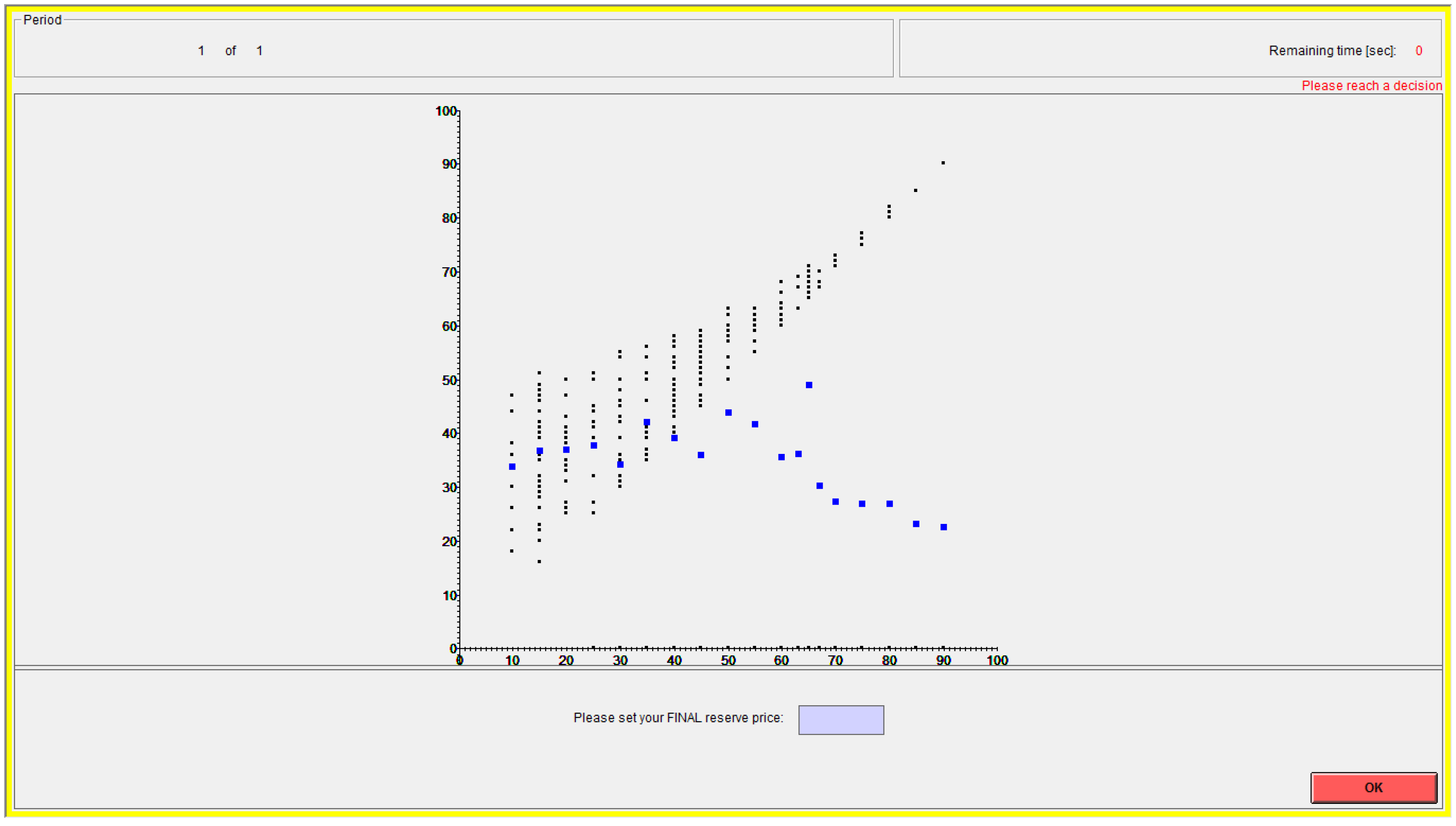
The subject had to choose a reserve price. The program on receiving the choice simulated an auction (generated bidder valuations, produced bids and determined outcome) and reported revenue earned. The subject was then paid a show-up fee of INR 50 and twice revenue earned, if any, in INR in private.2

Before making the final and payoff-relevant choice, the subject could practice on the same interface. Every time she/he entered a reserve price, the program would simulate an auction and display valuations, bids and outcome.3 It would also display this information graphically for every simulation, along with the history of past outcomes and the average (over all practice choices) revenue function (see Figure 1). The principal aim of the simulation tool was to aid the subject in constructing and solving hypothetical examples.

Treatment variables were the number of bidders and the length of the experience phase. There were either two or four bidders, and the phase-length was either 5 or 15 min. We denote the corresponding treatments as 205, 405, 215 and 415.

The experiment was conducted at the Institute for Management Technology, Ghaziabad, a business school near Delhi. There was one session per treatment, with registered subjects randomly allocated. Sessions lasted for between 30 and 45 min from the time subjects assembled to the time they left after payment. Subjects were students pursuing MBAs and were recruited through email solicitations and flyers. There were 37, 40, 35 and 39 subjects in Treatments 205, 405, 215 and 415, respectively.4

After subjects had assembled, each in front of a terminal, instructions (see Appendix A) had been handed out and read, numerical exercises done, and questions answered, and a demonstration was given of the interface to familiarize subjects with it. The experience phase commenced at the end of the demonstration, after the cessation of which, final and payoff-relevant reserve price choice had to be made.

4. Results

Our hypotheses, following the theoretical prediction described earlier, were that reserve prices chosen by subjects in every treatment were 50 on average and that choices did not differ across treatments.

$$Hypotheses:\{\begin{array}{c}A:r_i=50,i\in \{205,405,215,415\}\hfill \\ B:r_{205}=r_{405}=r_{215}=r_{415}\hfill \end{array}$$

where r is average observed reserve price and subscripts denote treatments.

4.1. Expected Revenues

Before presenting results from the tests of these hypotheses, we considered whether the expected revenue maximizing reserve price identified above might be a reasonable prediction when decisions were subject to sampling noise. Using $w=100$ and the uniformity of F in (2), the expressions for expected revenue relevant for our experimental treatments are:

$$\mathrm{\Pi }\left(r\right)=\left\{\begin{array}{cc}100(\frac{1}{3}+\frac{r^2}{{100}^2}-\frac{r^3}{75*{100}^2})\hfill & ifN=2\hfill \\ 100(\frac{3}{5}+\frac{r^4}{{100}^4}-\frac{2r^5}{125*{100}^4})\hfill & ifN=4\hfill \end{array}\right.$$

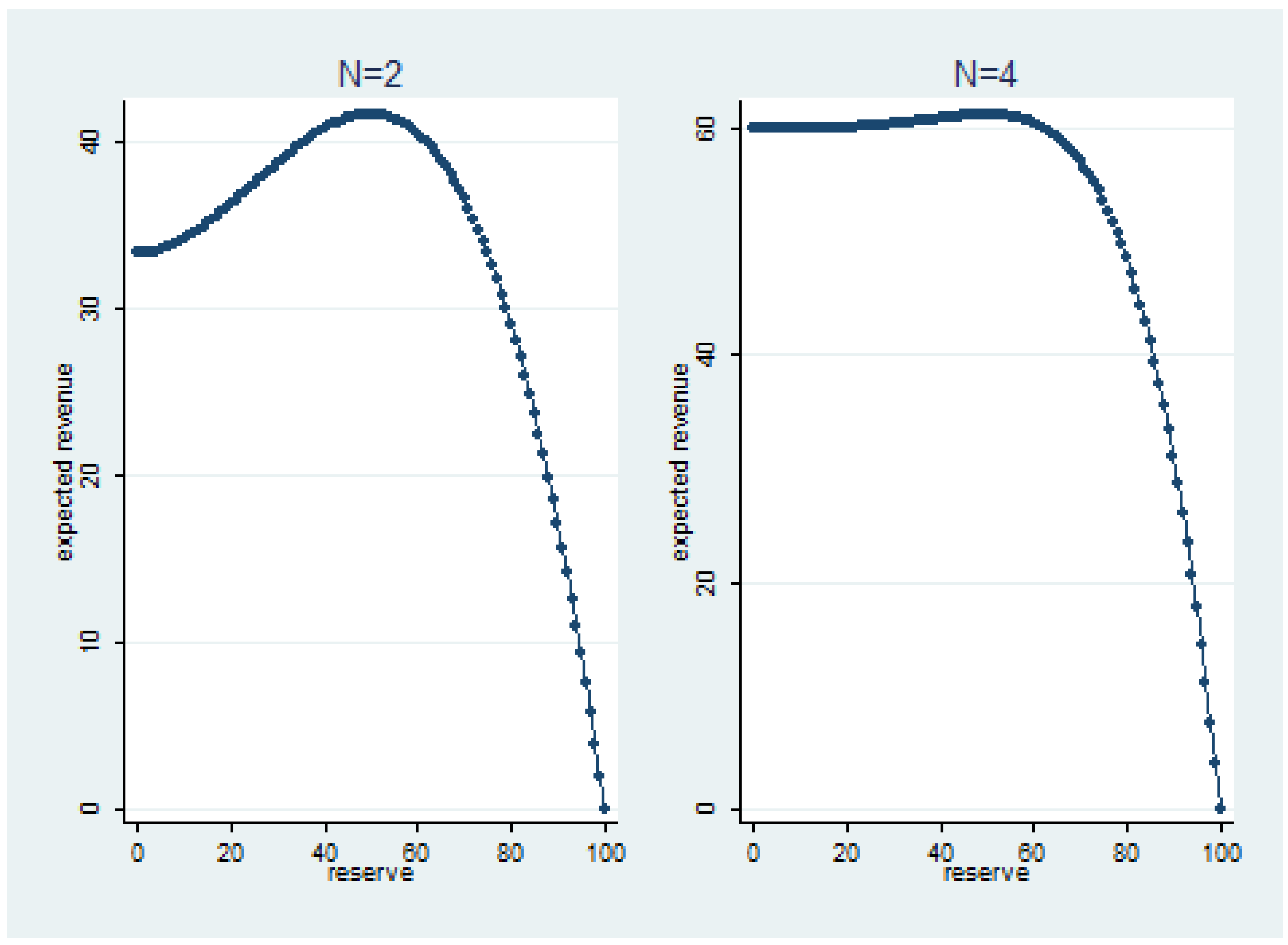
The plots of these functions are given in Figure 2.

The figure shows relatively flat regions around the peaks of the expected revenue functions, especially for $N=4$. This suggests that if subjects chose according to average revenue functions actually faced and if average revenue functions replicated expected revenue functions, it might have been quite hard to predict final reserve price choices on an a priori basis, particularly for $N=4$. Moreover, it would be difficult to attribute any failure of the hypotheses to a singular cause, as potential candidates could have inadequate learning capability, excessive sampling noise or simply that subjects did not care for insubstantial differences in revenue.

4.2. Reserve Prices Chosen

Table 1. Means and medians: reserve price.

Treatment	205	405	215	415
Mean	31.73	40.4	45.89	49.23
t-Test	<0.0001 ***	0.0028 **	0.1466	0.8142
Median	35	42	47	53
Wilcoxon Test	<0.0001 ***	0.0082 **	0.1294	0.9055

** and *** denote significance respectively at the 1% and 0.1% levels.

gives the mean and median final reserve prices for every treatment. It also presents two-tailed p-values from the tests of the hypotheses that these equal 50, the predicted value.

We found that with more experience average reserve prices were indistinguishable from 50 (Columns 3 and 4). Hypothesis A was thus upheld in Treatments 215 and 415. Average reserve prices were lower than the predicted value, however with less experience (Columns 1 and 2). Hypothesis A was hence rejected for Treatments 205 and 405.

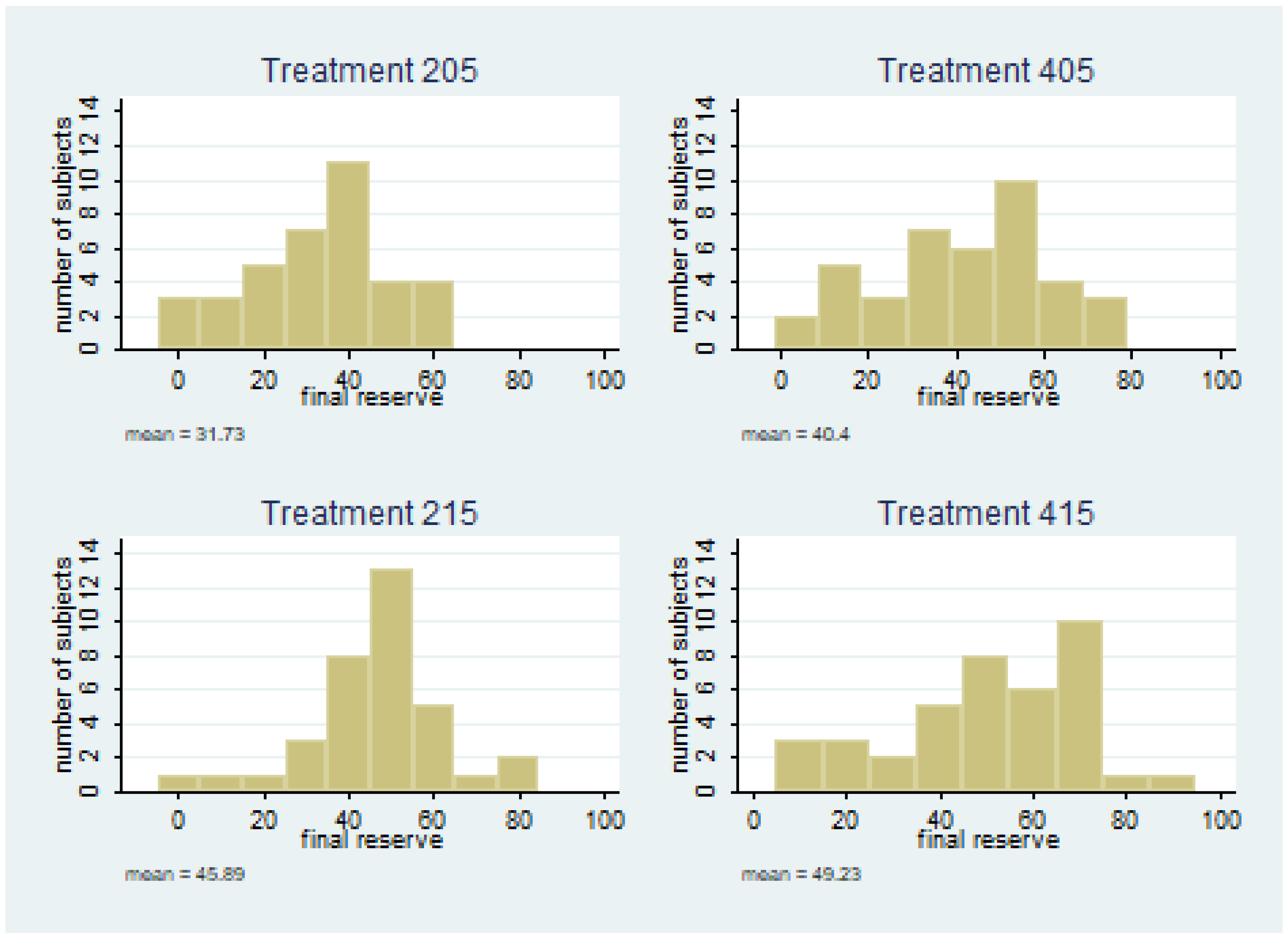
We also studied how dispersed final reserve choices were. Standard deviations of choices were 16.75, 19.06, 16.38 and 20.3 in Treatments 205, 405, 215 and 415, respectively. Figure 3 presents histograms of final reserve prices for each treatment. Overall, dispersion was fairly even, with little difference across treatments (see Section 4.4 for further discussion on this point), though choices appeared less clustered around the mean for treatments with our bidders.

4.3. Univariate Treatment Comparisons

Table 2. Treatment comparison tests: reserve price.

Comparison	205/405	205/215	405/415	215/415
t-Test	0.0379 *	0.0005 ***	0.0497 *	0.4412
Mann–Whitney Test	0.0321 *	0.0005 ***	0.0442 *	0.2334

* and *** denote significance respectively at the 5% and 0.1% levels.

gives two-tailed p-values from tests comparing average reserve prices across treatments. Only the main comparisons, focusing on marginal effects of the treatment variables, are given.5 The table shows that even with the problem of conjecturing bidder strategies eliminated by design, choosing the reserve price optimally remains a challenge, and more experience can aid in promoting better choice. We found that reserve price chosen by more experienced sellers did not depend on the number of bidders (Column 4), as predicted.6 Hypothesis B was upheld in the comparison between Treatments 215 and 415. It failed however in all other main treatment comparisons. Reserve price increased with the number of bidders for less experienced sellers (Column 1), which was inconsistent with the benchmark.7 Furthermore, reserve price appeared to increase with experience (Columns 2 and 3).

Table 1 and Table 2 thus show that our benchmark hypotheses were satisfied for more experienced subjects (Treatments 215 and 415). The reserve prices they chose were not dependent on average on the degree of competition as proxied by the number of bidders in the market, and moreover were statistically equal to 50, the predicted level. The behavior of less experienced bidders however failed to conform to the benchmark theoretical predictions. Their reserve price choices increased in the number of bidders and on average were shaded below the predicted level. Overall, Table 1 and Table 2 show that the degree of experience could be a predictor of choice, with choice indistinguishable from prediction with more experience, but distinguishable with less.

4.4. Average Revenues and Reserve Prices Chosen

The results presented above indicate that the concerns outlined in Section 4.1 are unwarranted. Subject choices in the high experience treatments, even with $N=4$, corresponded to theoretical predictions, while those in the low experience treatments, whether for $N=2$ or $N=4$, did not. These findings suggest that the failure of the hypotheses in the low experience treatments stemmed from inadequate learning, rather than any other cause.

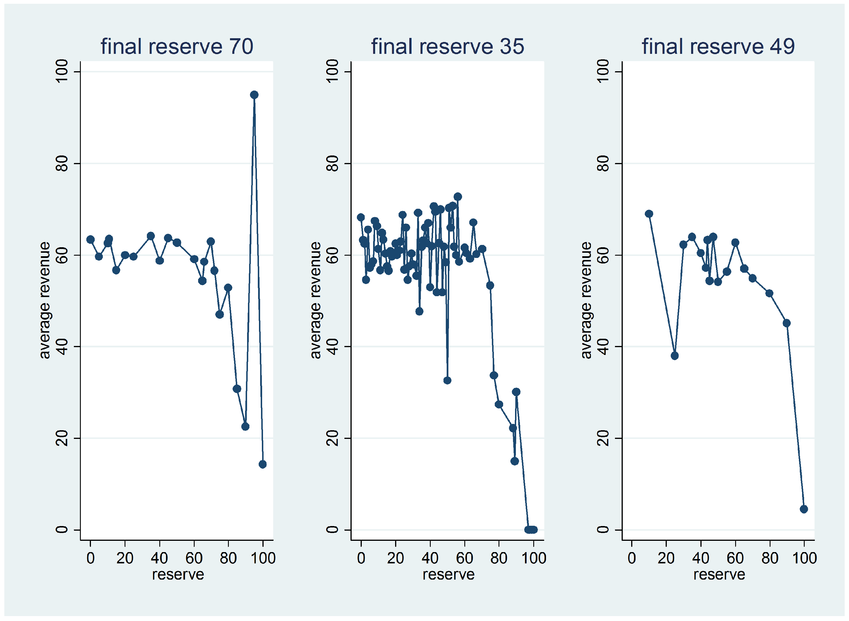
To investigate why choices in the high experience treatments corresponded to theoretical predictions, in spite of the relative flatness of the expected revenue functions noted earlier, we studied average revenues actually faced by subjects. Figure 4 plots average revenue functions for the three subjects with the highest number of practice choices. They all happened to be from treatment 415.

Three features stood out from an inspection of these average revenues. Firstly, average revenue functions were very jagged and replicated neither the smoothness, nor, for the most part, the exact shape of the expected revenue functions. Secondly, subjects did not necessarily choose all possible reserve prices during the practice phase. In the third panel in the figure, for example, most choices were concentrated around the benchmark optimal level. Thirdly, subjects did not necessarily seem to be always following average revenues exactly in determining final choice. To see this, note that the reserve prices giving the two highest average revenues were, from left to right in the figure, 95 and 35, 56 and 53, and 10 and 47, while the corresponding final reserve price choices were 70, 35 and 49, respectively. This suggests that average revenues were being used as a referent, rather than an exact determinant, with considerable heterogeneity across subjects, and could be because subjects were accounting for the presence of sampling noise. Overall, our findings indicate that while calculations based on expected revenues need modification for empirical application at the level of the individual subject, sufficient learning led to a concentration around the optimal level, despite the presence of sampling noise, heterogeneity and relative flatness of expected revenues.

It is of interest nevertheless to inquire whether the flatness of the expected revenues had any impact. While theory is of limited guidance here, a possibility that presents itself is that final reserve price choices will be more diffuse in the four-bidder case. We examine this proposition for the high experience treatments, which were directly comparable as they had indistinguishable means. We found weak support through a variance comparison test. Standard deviations were calculated to be 16.4 and 20.3 for 215 and 415 respectively, and a robust test for equality of variances showed that these were different at the 10% level (two-tailed p-value using the W50test statistic = 0.084).8

4.5. Obtaining Information through Practice

Results presented above in Section 4.2 and Section 4.3 suggest that subjects in the high experience treatments, with more opportunities to practice and acquire information, learned better and chose reserve prices closer on average to the level predicted by benchmark theory. A question is whether the degree of experience could be captured by the number of practice choices during the experience phase, where the number of practice choices was a measure of the amount of information obtained.

Table 3. Means, medians and comparison tests: number of practice choices.

Treatment	205	405	215	415
Mean	90.5	77.2	126.3	277.7
Median	85	63	131	223
Comparison	205/405	205/215	405/415	215/415
t-Test	0.1285	<0.0001 ***	<0.0001 ***	<0.0001 ***
Mann-Whitney Test	0.1094	0.0005 ***	<0.0001 ***	<0.0001 ***

*** denotes significance at the 0.1% level.

gives mean and median numbers of such choices along with two-tailed p-values from tests comparing these across treatments. We found that the number increased with the length of the phase (Columns 2 and 3). For less experienced sellers, the numbers did not depend on the number of bidders (Column 1).9 For more experienced sellers, the number of choices was increasing in the number of bidders (Column 4).10

Results in Section 4.3 and Table 2 (see also Section 4.6, and

Table 4. Treatment comparison regressions: reserve price.

Comparison	205/405	205/215	405/415	215/415
Treatment Dummy	8.3982 * (4.1914)	14.7005 ** (4.5823)	5.2955 (6.1263)	0.3087 (5.3058)
Number of Practice Choices	−0.0204 (0.0548)	−0.0152 (0.0657)	0.0176 (0.0211)	0.02 (0.0203)
Constant	33.5725 *** (5.7846)	33.1075 *** (6.5463)	39.0403 *** (3.5157)	43.354 *** (4.0536)

Standard errors are in parentheses. *, ** and *** denote significance respectively at the 5%, 1% and 0.1% levels.

and

Table 5. Regressions: Pooled data.

Dependent Variable	Final Reserve	No. of Practice Choices
dumN (0 if $N=2$, 1 if $N=4$)	5.713 (3.1892)	67.3519 *** (14.6553)
dumphase (0 if 5 min, 1 if 15 min)	10.736 ** (3.6132)	122.0284 *** (14.6424)
number of practice choices	0.0052 (0.0167)	- (-)
constant	32.8324 *** (2.7234)	48.5834 *** (12.7681)

Standard errors are in parentheses. ** and *** denote significance respectively at the 1% and 0.1% levels.

below) suggest that a longer phase allows greater experimentation in terms of selection of an individually suited search strategy, collection of more problem-related input data and superior analysis of collected data given any set of interim or final data collected. As an alternative hypothesis, one can suppose that a longer phase allows only better calculation, without any change in the stock or type of data on which calculations may be based, or the ability to calculate. Since pure and final calculation can only occur after collection of all data, a test can be devised that can help select amongst the hypotheses. Under the ‘calculations only’ hypothesis, a change in experimental conditions that leads to a movement toward optimality of chosen reserve price (increase in length of the phase) should not lead to a change in the quantum of data collection (number of practice choices). Positive correlation is expected however under our hypothesis. Findings in Table 3 (see also Table 5) rejected the alternative hypothesis in favor of ours, as an increase in the length of the phase led to a steep increase in the number of practice choices.

Regression analysis (not reported) revealed that once treatment differences were controlled for, the amount of information obtained did not predict choice or its distance from the optimum. This indicates that variation in the length of the experience phase may have been inducing learning strategies whose power could not be fully measured by the amount of information obtained. For example, a longer experience phase, by relaxing a resource constraint, could be inducing strategies with greater deliberation conditional on information acquired.

4.6. Multivariate Treatment Comparisons

A consequent question is if treatment comparisons for reserve prices hold when the amount of information obtained is controlled for. Table 4 gives results of linear regressions comparing average reserve prices across treatments with the amount of information obtained (number of practice choices) used as a control variable. The dependent variable was final reserve price chosen. A treatment dummy, which took the value zero or one, was also used. This variable took the value zero for 205, 205, 405 and 215 in the first, second, third and fourth regression, respectively.

We found that the amount of information obtained was never significant, and the univariate results reported above in Table 2 were mostly upheld. The exception comes from the comparison between 405 and 415, where reserve prices were no longer different. This weakens the finding from Table 2 above that reserve price chosen increased with experience.

The finding remains intact however when we conducted the analysis after pooling the data, as Column 1 of Table 5 shows. The table reports output from two linear regressions. The dependent variable for the first (Column 1) is final reserve price chosen, and the dependent variable for the second (Column 2) is the number of practice choices. There were two dummies used as independent variables for both regressions. One was for the number of bidders (dumN, taking the value one if the number was four, and zero otherwise), and the other was for the length of the phase (dumphase, taking the value one if the length was 15 min, and zero otherwise). The first regression included the number of practice choices as an independent variable.

Results from the first regression show that N, the number of bidders, did not have a significant impact, while phase length was significant (p-value = 0.003). The latter result supports the finding from Table 2. Results from the second regression show that an increase in phase length led to a large increase in the number of practice choices (p-value < 0.0001). This confirms the rejection of the ‘calculations only’ hypothesis discussed above (see Section 4.5).

5. Behavior of Less Experienced Sellers

We found that choices of more experienced sellers were consistent with the benchmark. Choices of less experienced sellers were lower than predicted, and increased with the number of bidders. In this section, we show that this pattern is consistent with the benchmark augmented with a probability weighting model. This indicates the possibility that the benefits of increased experience are expressed mainly as lower errors in probability assessment (e.g., Kahneman and Tversky 1979 [12]).

The general idea of probability weighting is that decision makers behave as if the probabilities of certain events are different from their given values. As in the literature (see, e.g., Wu and Gonzalez 1996 [13]), we assume there is a weighting function $w\left(p\right)$, mapping actual probability of occurrence to $[0,1]$, with (i) $w\left(0\right)=0$ and $w\left(1\right)=1$ and (ii) $w^{\prime }\left(p\right)>0$ for all $p\in [0,1]$.11 (i) implies that probabilities of events with probability zero or one will not get distorted through weighting. (ii) implies that events with higher probabilities will receive higher weights.

To proceed, we assume sellers distort the actual cumulative probabilities p of some events and represent them as $w\left(p\right)$ instead when performing expected revenue calculations. To express this formally, let $Y_1^{\left(N\right)}(.)$ and $Y_2^{\left(N\right)}(.)$ be respectively the distribution functions of the highest and second-highest order statistics of the N random variables ${\left(X_i\right)}_{i=1}^N$ and denote the derivatives of these two functions by $y_1^{\left(N\right)}(.)$ and $y_2^{\left(N\right)}(.)$, respectively. First suppose there is no probability weighting. The seller’s equilibrium expected revenue, given earlier in (2), can be written as:

$$\mathrm{\Pi }\left(r\right)=r[Y_2^{\left(N\right)}\left(r\right)-Y_1^{\left(N\right)}\left(r\right)]+{\int }_r^{w}zd{Y}_2^{\left(N\right)}\left(z\right)$$

(4)

The optimal or revenue maximizing reserve price can be determined using (4). The first order condition yields the following equation governing the optimal reserve price $r^{*}$ (the rule is the same as given earlier in (3), but expressed differently):

$$r^{*}=\frac{Y_2^{\left(N\right)}\left(r^{*}\right)-Y_1^{\left(N\right)}\left(r^{*}\right)}{y_2^{\left(N\right)}\left(r^{*}\right)-[y_2^{\left(N\right)}\left(r^{*}\right)-y_1^{\left(N\right)}\left(r^{*}\right)]}=\frac{1-F\left(r^{*}\right)}{f\left(r^{*}\right)}$$

(5)

We now incorporate probability weighting into the seller’s expected revenue function. (4) and (5) then respectively get modified as follows.

$$\begin{array}{ccc}\hfill \mathrm{\Pi }\left(r\right)& =& rw(Y_2^{\left(N\right)}\left(r\right)-Y_1^{\left(N\right)}\left(r\right))+{\int }_r^{w}zdw\left(Y_2^{\left(N\right)}\left(z\right)\right)\hfill \end{array}$$

(6)

$$\begin{array}{ccc}\hfill r^{*}& =& \frac{w(Y_2^{\left(N\right)}\left(r^{*}\right)-Y_1^{\left(N\right)}\left(r^{*}\right))}{y_2^{\left(N\right)}\left(r^{*}\right)w^{\prime }\left(Y_2^{\left(N\right)}\left(r^{*}\right)\right)-[y_2^{\left(N\right)}\left(r^{*}\right)-y_1^{\left(N\right)}\left(r^{*}\right)]w^{\prime }(Y_2^{\left(N\right)}\left(r^{*}\right)-Y_1^{\left(N\right)}\left(r^{*}\right))}\hfill \end{array}$$

(7)

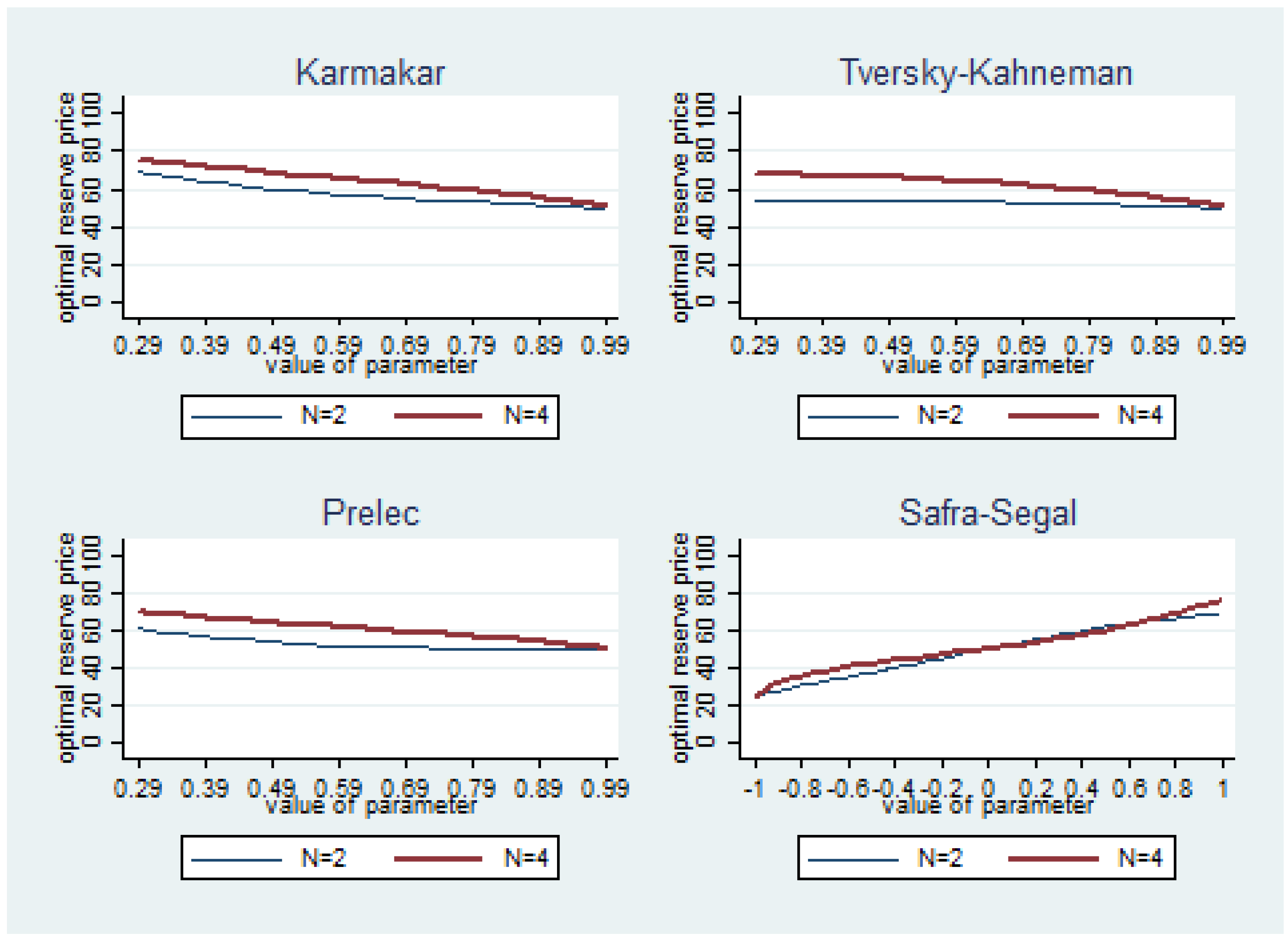
We can now apply (7) to predict optimal reserve price choices, provided we assume a specific form for $w(.)$. We look at four alternative single-parameter families: the Karmakar function (Karmakar 1978 [14], 1979 [15]), the Tversky–Kahneman function (Tversky and Kahneman 1992 [16]), the Prelec function (Prelec 1998 [17]) and the Safra–Segal function (Safra and Segal 1998 [18]), which are given sequentially below.

$$\begin{array}{ccc}\hfill w^K\left(p\right)& =& \frac{p^{\alpha }}{p^{\alpha }+{(1-p)}^{\alpha }},\alpha \in (0,1)\hfill \end{array}$$

(8)

$$\begin{array}{ccc}\hfill w^{TK}\left(p\right)& =& \frac{p^{\alpha }}{{[p^{\alpha }+{(1-p)}^{\alpha }]}^{\frac{1}{\alpha }}},\alpha \in (0,1)\hfill \end{array}$$

(9)

$$\begin{array}{ccc}\hfill w^P\left(p\right)& =& e^{-{(-lo{g}_{e}p)}^{\alpha }},\alpha \in (0,1)\hfill \end{array}$$

(10)

$$\begin{array}{ccc}\hfill w^{SS}\left(p\right)& =& p+\alpha p-\alpha p^2,\alpha \in [-1,0)\cup (0,1]\hfill \end{array}$$

(11)

The derivatives of these functions are as follows.

$$\begin{array}{ccc}\hfill \frac{d{w}^K\left(p\right)}{dp}& =& \frac{\alpha p^{\alpha -1}}{p^{\alpha }+{(1-p)}^{\alpha }}-\frac{\alpha p^{\alpha }[p^{\alpha -1}-{(1-p)}^{\alpha -1}]}{{[p^{\alpha }+{(1-p)}^{\alpha }]}^2}\hfill \end{array}$$

(12)

$$\begin{array}{ccc}\hfill \frac{d{w}^{TK}\left(p\right)}{dp}& =& \frac{\alpha p^{\alpha -1}}{{[p^{\alpha }+{(1-p)}^{\alpha }]}^{\frac{1}{\alpha }}}-\frac{p^{\alpha }[p^{\alpha -1}-{(1-p)}^{\alpha -1}]}{{[p^{\alpha }+{(1-p)}^{\alpha }]}^{(1+\frac{1}{\alpha })}}\hfill \end{array}$$

(13)

$$\begin{array}{ccc}\hfill \frac{d{w}^P\left(p\right)}{dp}& =& \frac{\alpha {(-lo{g}_{e}p)}^{\alpha -1}}{p}{e}^{-{(-lo{g}_{e}p)}^{\alpha }}\hfill \end{array}$$

(14)

$$\begin{array}{ccc}\hfill \frac{d{w}^{SS}\left(p\right)}{dp}& =& 1+\alpha -2\alpha p\hfill \end{array}$$

(15)

We calculated optimal reserve prices (rounded to the nearest integer) using (7)–(15) for $N=2$, as well as $N=4$, for all values of parameter $\alpha$ in $[0.29,0.99]$ with a grid increment of 0.01 for the K, TK and Pfunctions and all values of parameter $\alpha$ in $(-1,0)\cup (0,1)$ with a grid increment of 0.01 for the SSfunction. We chose this range for $\alpha$ for the first three functions because it is within most range estimates found in prior literature. Further, we got a unique solution for all values of $\alpha$ in this range, while the use of the TK function led to non-uniqueness for $\alpha <0.29$.12

Our results are summarized in Figure 5. For the K, TK and P functions, we found that probability weighted optimal reserve prices are no less and usually higher than the unweighted benchmark. These functions are thus unable to concur with our finding that less experienced sellers tend to choose lower than benchmark reserve prices. Concurrence is generated though by the SS function, which predicts a probability weighted optimal reserve price less than 50, for parameter values $\alpha <0$. We further found that the K, TK and P functions yield the prediction that sellers should choose higher reserve prices when the number of bidders is greater. This is in consonance with our finding. The SS function generates the same prediction for $\alpha <0$ and also for $\alpha >0.69$. Overall, therefore, the SS function seems most applicable to our data as, for $\alpha \in (-1,0)$, it predicted both that reserve prices should be lower than the unweighted benchmark and that the price should increase in the number of bidders.

6. Conclusions

Prior studies showed using a standard learning protocol that reserve price choices of laboratory sellers may not be independent of the number of bidders. We found that a modified version of an alternative protocol proposed by Merlo and Schotter (1999) [4] can foster learning if sufficient opportunity for gathering experience is allowed.13 The amount of information obtained increased with the opportunity to gather experience. Choices of more experienced sellers coincided with the optimal decision defined by the problem and were independent of the number of bidders. Less experienced sellers chose reserve prices that were lower than the optimum and increasing in the number of bidders. There was some evidence that reserve price chosen increased with experience. Analysis of how learning is modified when obtaining information or increasing the length of the experience phase is costly may be of future research interest.