Article

The Effect of Competition on Risk Taking in Contests

1
Department of Economics and Statistics, University of Siena, 53100 Siena, Italy
2
Department of Economics and CentER, Tilburg University, 5000 LE Tilburg, The Netherlands
*
Authors to whom correspondence should be addressed.
Games 2018, 9(3), 72; https://doi.org/10.3390/g9030072
Submission received: 15 July 2018 / Revised: 14 September 2018 / Accepted: 17 September 2018 / Published: 19 September 2018
(This article belongs to the Special Issue Economic Behavior and Game Theory)

Abstract

:
We investigate, theoretically and experimentally, the effect of competition on risk taking in a contest in which players only decide on the level of risk they wish to take. Taking more risk implies a chance of a higher performance, but also implies a higher chance of failure. We vary the level of competition in two ways: by varying the number of players (2 players versus 8 players), and by varying the sensitivity of the contest to differences in performance (lottery contest versus all-pay auction). Our results show that there is a significant interaction effect between the two treatments, suggesting that players are particularly prone to take more risks if both the number of players and the sensitivity to performance are higher.

1. Introduction

Both in markets and in sports, players often compete for a single prize, be it a contract, an innovation, or a medal. Such settings are usually modeled as contests in which players can expend resources, such as effort, money, or time, to win a prize.1 Players trade off the cost of the resource against an increased probability of winning the prize. In this paper, we do not focus on the level of resources players expend, but rather, on the level of risk they take. By taking more risk, players can willingly increase the variance of possible outcomes. Rather than playing safe, a player can increase the possibility that something good happens at the expense of an increase in the probability that something bad happens.
An example of this kind risk-taking is choosing the difficulty level of an exercise in figure skating or gymnastics. By choosing a higher difficulty level, the athlete wins more points if the exercise is well-executed; however, the probability of failure also increases. Another case in point is swerving and elbowing during a cycling sprint, which can generate a competitive edge, but also increases the risk of a crash. In finance, one can think of a fund manager who chooses the riskiness of an investment portfolio in the face of tournament-based performance rewards. In academia, a job market candidate may affect the level of risk by submitting a paper to a top core journal rather than a good field journal. Doing so gives a shot at an exceptionally good outcome, but also increases the probability of painful rejection. Notice that in each of these cases, the level of risk is a decision variable of the agent.2
We are not first to study risk taking as a strategic variable in contests. Bronars [3] shows that leaders in a sequential tournament have an incentive to choose low risk levels, while laggards will tend to choose a high-risk strategy. Hvide [4] considers a model with both effort and risk as decision variables and shows that the possibility to affect risk (variability) may dilute the incentive to provide effort. Gilpatric [5] extends this analysis and shows how such harmful incentive effects of risk taking can be remedied with a carrot and stick policy. Gaba et al. [6] focus on contests with multiple winners and show that equilibrium levels of risk taking will be high (low) when the number of winners is relatively low (high).
Our main research question is whether levels of risk taking are affected by the competitiveness of the contest. If it becomes harder to ‘beat’ your opponents, will this induce you to take more risk in an attempt to attain an exceptionally good performance? We explore this question both theoretically and experimentally.
We analyze a contest in which players compete for a single prize. The probability to win the prize depends positively on the performance of a player. Each player decides how much risk to take, where there is a trade-off between the level of performance and the probability of attaining that performance. Specifically, a player chooses a level of risk f between zero and one, and performs at level f with probability 1 − f and at level 0 with probability f. This method for implementing risk taking is introduced by Crosetto and Filippin [7]. It is referred to as the Bomb Risk Elicitation Task, where the ‘bomb’ relates to the bad outcome occurring with probability f. This type of risk taking corresponds closely to the examples we discussed above, such as the athlete choosing the difficulty level of an exercise or the researcher deciding which journal to submit a paper to.
We vary the level of competition in two different ways. One is by varying the number of players in the contest. As we will illustrate by means of numerical analysis below, increasing the number of players increases the equilibrium level of risk taking. The second variation of competition we analyze is the sensitivity of the contest to differences in performance. A case in point would be an increase in the discriminative quality of the jury in gymnastics, due to which objective performance becomes more important and noise is reduced. In one version of the contest, we consider the probability to win the prize is proportional to performance (such as in a lottery contest); in the other version of the contest, the prize is assigned to the player with the highest performance (such as in an all-pay auction). In the latter version, only the best performance is rewarded and, as we will illustrate below, the corresponding equilibrium involves a higher expected level of risk taking than the former version in which even suboptimal performers have a chance to win the prize.
Based on the theoretical analysis, we hypothesize that levels of risk taking in a contest will (1) increase with the number of players competing for the prize, and (2) be higher if the prize is assigned to the player with the best performance (all-pay auction) as compared to the case in which winning probabilities are proportional to performance (lottery contest). We implement an experiment to test these hypotheses. The experiment is designed similar to the contest model described above. Subjects must decide to open anywhere between 1 and 100 boxes. One random box contains a red chip; each of the other 99 boxes contains a green chip. Who wins the prize depends on the number of green chips collected. When a subject collects the red chip, all green chips are destroyed and a penalty has to be paid. We implement a 2 × 2 design in which (a) the number of players is either 2 or 8, and (b) the prize is assigned either to the player who collected the highest number of green chips (all-pay auction), or to the owner of one green chip which is randomly drawn from all green chips collected by all players (lottery contest).
Our experimental results do not provide unequivocal support for the two hypotheses. For the lottery contest, we find no support for the hypothesis that the average levels of risk taking are higher with 8 players than with 2 players. At the same time, for the all-pay auction we do find support for the same hypothesis. Here, the average levels of risk taking are significantly larger with 8 players than with 2 players. Similarly, for the 2-player case, we find no support for the hypothesis that risk levels are higher in the all-pay auction than in the lottery contest. For the 8-player case, however, we do find significant support for the same hypothesis. The combination of these results, indicates that there is a significant interaction effect between the number of players in a contest and the sensitivity of the contest to performance differences. Even though we had not hypothesized such an interaction effect, in retrospect, we can see that it is much in line with the equilibrium predictions. Still, observed levels of risk-taking deviate from the benchmark equilibrium levels on several accounts. We discuss to what extent these can be explained by behavioral factors, such as risk aversion, loss aversion, collusion, bounded rationality, and learning. The latter factor seems to provide the best account for the behavioral patterns we observe.

2. Related Literature

There are only a few studies that use field data to investigate the relationship between risk taking and competition. Bothner et al. [8] use data on car crashes in NASCAR races as a proxy for risk taking. They find that drivers are more likely to crash their vehicle when they face fiercer competition from nearby counterparts. This suggest that competitive pressure increases risk taking. The influence of competition on risk taking behavior has also been analyzed in fields such as innovation [9,10], and banking [11,12]. Again, the evidence suggests a positive effect of competition on risk taking. However, establishing causality is complicated by endogeneity issues. That is why we use an experiment, which allows for the degree of competition to be varied exogenously. Another reason is that experiment risk taking behavior can be observed directly and does not need to be proxied.
There is an extensive experimental literature on contests, and the treatment variations we implement are not novel. Some experimental studies have examined the effect of different contest structures [13,14,15]. In line with theoretical predictions, it is found that effort levels are higher in all-pay auctions than in lottery contests. We implement a very similar treatment comparison, but we focus on risk taking rather than on effort provision.
Several experimental papers study the effect of the number of players on effort levels in contests, including lottery (Tullock) contests [16,17], all-pay auctions [18,19], and rank-order tournaments [20,21]. As discussed in Dechenaux et al. [1], the results are somewhat mixed, but overall the evidence seems to point at a negative relationship between group size and individual effort levels. Dechenaux et al. (2015) [1] offer a review of the experimental research about contests. Konrad (2009) provides a survey of the theoretical literature.
Whether a similar result holds for levels of risk taking is an open issue, because effort levels cannot be easily translated to risk levels.
The experimental study closest to ours is Eriksen and Kvaløy [22]. They examine risk taking in tournaments where the optimal strategy is to take no risk, irrespective of the level of competition. They find that subjects take excessive levels of risk which, moreover, increase with the level of competition. The tournament they implement is different from the contest we study. Also, the way they implement risk taking is different from ours. They adopt a version of the lottery investment task introduced by Gneezy and Potters [23], while we employ the “Bomb Risk Elicitation Task” introduced by Crosetto and Filippin [7]. Another relevant difference is that in Eriksen and Kvaløy [22] the equilibrium is a corner solution with no risk taking. Any deviation from equilibrium then points at excessive risk taking. In our game, equilibrium involves an interior solution. This means that deviations from equilibrium can involve both too much and too little risk taking.

3. Theoretical Analysis

The experiment is based in the following contest. Let yi be the performance of player i, where i { 1 ,   ,   n } . The probability that player i wins a prize of value v is given by the following standard contest success function:
p i = y i r j = 1 n y j r
where r measures the sensitivity of winning probabilities to differences in performance. With r = 0, winning probabilities are unrelated to performance; with r = 1 they are proportional to performance, and when r → ∞ the player with the highest performance wins the prize (and random assignment in case of a tie). Contests based on the general form of the contest success function (for arbitray r) are usually referred to as Tullock contests. The case r = 1, corresponds to, what is often called, a lottery contest; for r → ∞ the Tullock contest converges to an all-pay auction [1] and we will retain that terminology. Our analysis focuses on these two canonical contest types.
Performance is endogenous and determined as follows. Player i’s decision variable is fi and it affects performance as follows:
y i = { f i w i t h   p r o b a b i l i t y   1 f i 0 w i t h   p r o b a b i l i t y   f i
where 0 < fi ≤ 1 measures the degree of risk taking.3 If the bad outcome, yi = 0, materializes (which happens with probability fi) the player also incurs a negative payoff of −c, which we think of as the cost of a crash. Note that expected performance E (yi) is maximized at fi = ½. However, players may decide to choose a level of risk, fi < ½, in order to reduce the probability of incurring the cost of a crash. Conversely, players may decide to choose a higher level of risk, fi > ½, in order to have a shot at a higher level of performance, translating into a higher chance to win the prize v.
Contests are notoriously difficult to solve analytically, especially for all-pay auctions with r → ∞ [24]. In our analysis, we focus on symmetric equilibria. This allows us to express the expected payoff of a player under the assumption that all other players play the same strategy (which we will label f i ). Another assumption we make is that players are risk-neutral. With a prize equal to v, and the cost of a crash equal to c, player i’s expected payoff from playing f i , given that the other players play f i , can then be expressed as follows:
π i ( f i , f i ) = v { [ j = 1 n ( f i ) r ( f i ) r + ( n j ) ( f i ) r ( 1 f i ) ( 1 f i ) n j ( f i ) j 1 ( n 1 ) ! ( n j ) ! ( j 1 ) ! ] + f i ( f i ) n 1 n } c f i
The summation (from j = 1 to n) considers all scenarios in which player i does not crash while anywhere between 0 (j = 1) and n − 1 (j = n) of the other players do not crash either. The term ( f i ) r ( f i ) r + ( n j ) ( f i ) r is the probability that player i wins the prize in each of these scenarios and ( 1 f i ) ( 1 f i ) n j ( f i ) j 1 represents the probability that player i does not crash, nj others do not crash either, while j − 1 others do crash. The term ( n 1 ) ! ( n j ) ! ( j 1 ) ! is the number of permutations with j − 1 players crashing among n − 1 competitors. f i ( f i ) n 1 n is i’s probability of winning the prize for the scenario in which all the players crash (including i). Finally, c f i is the expected cost of crashing.
We will focus on a discrete version of the game in which strategies fi are represented by the set {0.01, 0.02, …, 0.99, 1}.4 For our contest we mainly rely on numerical methods to find the Nash equilibria.5 Specifically, we use a quasi-Newton technique to find the mixed strategy equilibria for the case r → ∞ [25]. This strategy grid corresponds to the strategies in the experiment (see below). For the case r = 1, the unique symmetric equilibria are in pure strategies. For values of n ranging from 2 to 10, these equilibria are presented in the second column of Table 1. For the case r → ∞ the equilibria are in mixed strategies. The third column of Table 1, displays the expected level of risk taking for these equilibria.
Based on these results we formulate the following two hypotheses.
Hypothesis 1 (number of players).
The level of risk taking (as measured by the average value of fi) increases with the number of players (n).
Hypothesis 2 (sensitivity to performance differences).
The level of risk taking (as measured by the average value of fi) is higher if the prize is assigned to the player(s) with the highest performance (r → ∞) than if the probability of winning the prize is proportional to performance (r = 1).

4. Experimental Analysis

4.1. Design and Procedures

Data were collected from 12 experimental sessions conducted in CentER lab at Tilburg University in September 2016. In total, 178 subjects participated, all students at the university and recruited via an online system.7 The experiment was programmed using z-Tree [26]. In a 2 × 2 between-subject design, subjects participated in contests with either n = 2 or n = 8 players, and with performance sensitivity of either r = 1 or r → ∞.8 At the beginning of each session, subjects were randomly and anonymously assigned to groups, which remained fixed throughout the experiment (partner matching).9 Written instructions were distributed (see Appendix B for a set of sample instructions). To allow for learning, each session consisted of 20 identical rounds.
In each round, participants competed for a prize (v) of 1000 Experimental Currency Units (ECU). The chance to win the prize depended on the number of “green chips” collected by each of the participants in the group. In the treatments with r = 1, subjects were informed that the probability to win the prize was equal to the number of green chips collected by them divided by the total number of green chips collected in their group. In the treatments with r → ∞, subjects were informed that the participant with the highest number of green chips would win the prize, and that the winner would be determined randomly in case of a tie.
To collect green chips, subjects had to choose how many “boxes” they wished to open. They were informed that there were 100 boxes, 99 containing a green chip and one containing a “red chip”. All boxes were equally likely to contain the red chip. If all boxes a participant opened contained a green chip, then that was how many green chips the participant collected. If one of the boxes contained the red chip the participant collected no green chips and incurred a penalty (c) of 50 ECU. If all participants in the group collected the red chip (i.e., no green chips were collected) the prize was randomly assigned.10
After all participants had entered how many boxes they wished to open, the computer randomly determined, for each participant separately, whether they had collected the red chip, and which of the participants had won the prize. At the end of the round, participants were informed about the number of boxes they had opened, whether or not they had collected the red chip, whether they had won the prize, and about their payoffs in ECU for the round. This information was also available in later rounds. Participants were not informed about the number of boxes opened or the number green chips collected by other participants.
After all of the 20 rounds were completed, the computer randomly selected one round for payment. ECUs were exchanged at a rate of 100 ECU for €0.80 in the treatments with groups of size 2 and at a rate of 100 ECU for €3.20 in the treatments with groups of size 8. This difference in exchange rate served to keep expected earnings more or less constant across treatments. Subjects also received a show-up fee of 5 Euro. They were told that any cost of collecting the red chip would be deducted from this show-up fee. At the end of the experiment, but before payment, the subjects were asked to fill in a brief questionnaire. It asked for their gender, age, their assessment of the level of complexity of the experiment, and their self-assessed measure of risk preference (as in Dohmen et al. [27]). From start to finish, an experimental session lasted about 45 min, and the average earnings were €8.40.

4.2. Results

Our main interest is in how risk taking varies with the competitiveness of the contest. We take the number of boxes opened by a subject in a round as the measure of risk taking. Below we will refer to this variable as the “bet”. A bet can take a value between 1 and 100, and a higher bet implies a higher level of risk. We will refer to the two treatment variables as “r” and “n”, where r can take values r = 1 and r → ∞, and n can take values n = 2 and n = 8.
Table 2 displays how the bets vary across the four treatments. The bets are averaged over all 20 periods and all players in a group, this provides us with one observation per group. The table also provides the number of groups in each treatment and the standard deviation of the mean bets across groups. From the column totals (i.e., pooling over treatments r = 1 and r → ∞) we can see that average bets increase with the number of players in a group from 36.92 with n = 2 to 42.86 with n = 8. The difference is significant at p = 0.044. From the row totals (i.e., pooling over treatments n = 2 and n = 8), we can infer that average bets increase with an increase in the sensitivity of winning probabilities, from 36.00 with r = 1 to 40.87 with r → ∞. The difference is significant at p = 0.069. So, there seems to be substantial support for the hypotheses formulated above.
The support for the hypotheses, however, is not unequivocal. In the row corresponding to r = 1, we see that average bets in treatment r = 1|n = 2 are not significantly different from those in treatment r = 1|n = 8 (and are actually somewhat lower in the latter treatment). Only in the row corresponding to r → ∞, we observe a significant increase in average bets when going from treatment r → ∞|n = 2 to treatment r → ∞|n = 8. Similarly, when we consider the rows corresponding to n = 2 and n = 8, respectively, we see that average bets are not significantly different between treatment r = 1|n = 2 and treatment r → ∞|n = 2, whereas average bets are significantly lower in treatment r = 1|n = 8 than in treatment r → ∞|n = 8. This suggests that there is an interaction effect between n and r. Increasing the number of players from n = 2 to n = 8 increases the average bets if and only if r → ∞, and, conversely, increasing the sensitivity from r = 1 to r → ∞ increases bets if and only if n = 8.
A closer look at Table 1 indicates that such an interaction effect is actually much in line with the equilibrium predictions. The difference in predicted average bets when going from r = 1 to r → ∞ is 0.20 if n = 2 (0.45−0.25) and 0.23 if n = 8 (0.61−0.38). Similarly, the difference in predicted average bets when going from n = 2 to n = 8 is 0.13 if r = 1 (0.38−0.25) and 0.16 if r → ∞ (0.61−0.45). So, even though we had not hypothesized such an interaction effect, it is in line with equilibrium. However, the interaction effect in the experiment is much larger than predicted by equilibrium. The difference in average bets when going from r = 1 to r → ∞ is 14.86 larger with n = 8 than with n = 2 [(50.97−37.68) − (34.76−36.33)], whereas this difference is predicted to be only 3. Similarly, the difference in average bets when going from n = 2 to n = 8 is 15.86 larger with r → ∞ than with r = 1 [(50.97−34.76) − (37.68−36.33)] whereas this is predicted to be only 3.
Besides looking at average bets, it is also instructive to look at the distributions of the bets and how these compare to the corresponding equilibria. A graphical display of this comparison is presented in Appendix A.3. For the treatments with a pure strategy equilibrium (r = 1|n = 2 and r = 1|n = 8) bets are quite dispersed and there is no indication that the equilibrium has any particular drawing power. For the treatments r → ∞|n = 2 and r → ∞|n = 8, the mixed strategy equilibria display a distinct shape with probabilities gradually increasing until a peak at bets of 67 and 77, respectively, and dropping off sharply at higher bets. However, this distinct shape is not visible in the data. At the same time, we do not find that the bets display a bi-modal distribution as is often found in the experimental contests with effort as the strategic variable (e.g., Gneezy and Smorodinsky [18]; Müller and Schotter [29]).11
We will now look at the evolution of the average bets over time. Figure 1 illustrates how average bets develop over the rounds for each of the four treatments. Average bets display a clear upward trend in treatment r → ∞|n = 8, whereas we observe a slight downward trend in the other three treatments. This dynamic pattern of the average bets reiterates the observed interaction between r and n. There is a discernible increase in the average level of risk taking if and only if both the number of players and the sensitivity to performance are higher.
To put these observations in perspective, we now conduct a multivariate analysis. Table 3 presents linear regressions in which the average bets are projected on the treatment variables, an interaction between the treatment variables, and the round number. First, we see that the significant positive effects of n = 8 and r → ∞ on average bets in model (1) disappear if we include the interaction between r → ∞ and n = 8 in model (2). This interaction effect is both sizeable (corresponding to 15 opened boxes) and significant. Second, we see an overall mild negative effect of the round number in model (3), but if we include an interaction with the treatment r → ∞|n = 8 we observe a positive time trend for this treatment.
Until now we have focused on average bets per group. These averages, however, may hide substantial heterogeneity across players. We now explore whether the differences in bets are related to the questionnaire data we collected about gender, age, perceived complexity of the game, and self-assessed risk attitude. Table 4 presents linear panel regressions in which a player’s bet in a round is related to treatment variables, the interaction between the treatment variables, the round number, and the individual background variables (female, age, perceived complexity, and proneness to take risk). Model (1) includes only the treatment variables and the round number, Model (2) adds the background variables, Model (3) also adds two variables that relate to subjects’ experience in the last period: whether they collected the red chip (L.redchip), and whether they won the prize (L.win).
The results from model (1) reiterate those from Table 3. We find no unilateral treatment effect, but a strong interaction effect. The results of model (2) indicate a gender effect where, as is often found, females tend to take less risk than males. The results also show that subjects who found the experiment complex entered higher bets, and the same holds for subjects who considered themselves to be prone to take risk. Model (2) also shows that controlling for these variables hardly affects the coefficients of the treatments.
Finally, Model (3) provides a glance at the dynamics of behavior. It turns out that subjects who draw the red chip in the last round tend to enter higher bets in the current round. This is quite remarkable. It suggests that subjects who have just had an ‘accident’ then go on to take more risk than those we did not have accidentally come upon the chip.12 The effect is reminiscent of the gambler’s fallacy—subjects believe that a random event is unlikely to happen again. Winning the contest does not have a significant effect on subsequent risk-taking, as can be seen from the insignificant coefficient of L.win. When we examine these response patterns for each treatment separately we find that the positive effects of both L.redchip and L.win are much larger in treatment r → ∞|n = 8. This may partially account for the positive time trend in that treatment (see Figure 1).

5. Discussion

One remarkable finding is that the average level of risk taking in treatment r = 1|n = 2 is higher than predicted by equilibrium, while the average levels of risk taking in the other three treatments are lower than predicted (see Figure 1). What might explain this? Natural candidates to consider are risk aversion and loss aversion. Effectively, both risk aversion and loss aversion increase the value of the cost of a crash (c) relative to the value of prize (v).13 It can be shown that this leads to lower predicted levels of risk taking. So, the presence of risk aversion and loss aversion may explain why observed levels of risk taking are lower than predicted by (risk neutral) equilibrium in all treatments, but not why it is below equilibrium in three treatments and above equilibrium in one treatment.14
Collusion may be another relevant factor, especially since subjects play the game repeatedly with the same opponent(s). Theory would predict that collusion can be sustained more easily if the gains from cooperation are large relative to the gains from defection. The experimental results are not in line with this prediction though. To illustrate, we compare treatment r = 1|n = 2 to treatment r → ∞|n = 2. Collusion implies taking as little risk as possible (fi = 0.01) and the corresponding payoffs are the same in the two treatments. The equilibrium payoffs are slightly lower in treatment r = 1|n = 2 than in treatment r → ∞|n = 2. At the same time, defecting from collusion is much less profitable in treatment r = 1|n = 2 than in treatment r → ∞|n = 2. In the former treatment (r → ∞), a marginally higher level of risk (fi = 0.02) suffices to win the prize almost certainly, whereas this is not the case in the latter treatment (r = 1) where winning probabilities are proportional to performance. These attractive defection payoffs erode the scope for collusion. From this perspective, we should expect collusion (bets below equilibrium) to be more prevalent in treatment r = 1|n = 2 than in treatment r → ∞|n = 2. However, the data suggest exactly the opposite (see Figure 1)—namely, that bets are above equilibrium in treatment r = 1|n = 2 and below equilibrium in treatment r → ∞|n = 2.15
An alternative explanation to consider is bounded rationality. It has often argued that Nash equilibrium relies on unrealistic assumptions about the cognitive abilities of players. One alternative solution concept we considered is the Cognitive Hierarchy (CH) model [30]. As it turns out, the CH model does perform somewhat better than Nash equilibrium in predicting the observed levels of risk taking in our experiment.16 In particular, CH predicts more or less the same average levels of risk taking than Nash equilibrium for the treatments with r = 1, and somewhat lower levels of risk taking in the treatments with r → ∞. Still, CH suffers from a similar problem as loss aversion and risk aversion. It does help to explain why observed levels of bets are below equilibrium in most treatments, but it does not explain why bets are above equilibrium in the treatment r = 1|n = 2 and n = 2.
Another way to look at the data displayed in Figure 1 is by focusing on the dynamics and disregarding the equilibria for the moment. First observe that the average bets in the first round are very similar across the four treatments, ranging roughly from 40 to 45. In first few rounds treatment differences are very small indeed, and statistically insignificant. Arguably, in the first rounds, the random component to behavior is still large, and it is only over time that treatment differences appear. Specifically, we observe a gradual increase of the bets in treatment r → ∞|n = 8, while there is a small decrease of bets in the other three treatments, especially in those with r = 1. What may cause these different developments over the rounds?
Basic learning dynamics such as reinforcement learning develop in accordance with subjects’ experiences. They depend on the feedback subjects receive on the relationship between their choices and their payoffs.17 Choices which generate relatively high payoffs are more likely to be played in subsequent rounds than choices which generate relatively low payoffs. So, we may hypothesize that average learning patterns will tend to develop in line with the empirically observed relationship between choices and payoffs. Figure 2 displays these relationships for each of the four treatments. They are based on simple regressions in which the realized payoffs of a subject in a round are estimated to be a quadratic function of his or her bet in that round.18
Now we relate the estimated relationship in Figure 2 to the behavioral patterns in Figure 1. In treatment r = 1|n = 2 (top-left panel) the maximum payoff is reached at a bet level of 15 which is substantially below the level of 40 at which the bets start.19 This may explain the downward trend we observe in this treatment. In treatment r → ∞|n = 8 (bottom-right panel) the maximum payoff is reached at about 90 which is much higher than in the other treatments and also much higher than the level at which the bets start in round 1. This may explain the upward time trend of the bets in treatment r → ∞|n = 8. In treatment r = 1|n = 8 (top-right panel), the maximum is reached at 50, which is somewhat higher than the level of 40 at which the bets start in round 1. Based on this we might expect an upward trend; instead we observe a slight downward trend. Finally, in treatment r → ∞|n = 2 (bottom-left panel) the empirical payoff maximum is reached at a bet of 35, which is close to the average bets in the first rounds. Consistent with this, we hardly see a time trend in this treatment.
So, even though the picture it not fully consistent, we may conclude that the aggregate dynamics of the bets can be explained reasonably well by a simple learning model in which the bets start more or less randomly, and then develop in line with the empirical relationship between bets and payoffs.

6. Conclusions

In this paper we examine the impact of competition on risk taking in contests. We vary the intensity of competition by varying the number of competitors (2 players versus 8 players) and by varying the sensitivity of winning probabilities to differences in performance (lottery contest with proportional winning probabilities versus all-pay auction with prize assigned to the highest performance). For our specific model, the Nash equilibrium predicts that players will take more risk when competition intensifies. Experimental results do not provide unambiguous support for the theoretical predictions, as the variations in the intensity of competition did not always have a significant effect on the levels of risk taking. However, in line with the prediction, we observe a significant interaction effect between the two treatments. If the prize is assigned to the player with the highest performance (all-pay auction), risk taking is higher with 8 players than with 2 players. Similarly, with 8 players, risk taking is higher with the all-pay auction than with the lottery contest.
Another remarkable result is that in three of the four treatments, we observe that subjects on average take less risk than predicted by the benchmark equilibrium. This result is in contrast to Eriksen and Kvaløy [22], who find that subjects tend to take excessive risk in comparison to the optimal strategy. Besides, in Eriksen and Kvaløy [23] the degree of risk-taking increases as the number of contestants grows, whereas in our experiment it is true only when the sensitivity to differences in performance is high. Our results also show that females are less prone to take risk than males, indicating that the well-known gender effect extends to competitive environments in which risk taking is a strategic variable.
Exploring the effect of competition on risk taking is a broad and promising topic, worthy of further research. It would be interesting to look at contests with different structures, such as contests with endogenous entry, and dynamic contests in which the degree of competition is to some extent endogenous. In such an environment, risk taking strategies may well depend on whether a player currently is a leader or a laggard, as well as on the degree to which the leader’s position is being threatened. Recently, there has been some progress on the theoretical analysis of dynamic contests and the role of interim information (e.g., Ederer [31]). We believe that this also offers a fruitful avenue for experimental inquiry.

Author Contributions

Conceptualization, J.P.; Data curation, J.P.; Formal analysis, L.S.; Funding acquisition, L.S.; Methodology, J.P.; Software, L.S.; Supervision, J.P.; Writing—original draft, J.P.

Funding

We would like to thank the Einaudi Institute for Economics and Finance for making this research possible by providing a grant to Spadoni.

Conflicts of Interest

The authors declare no conflict of interest. The funders had no role in the design of the study; in the collection, analyses, or interpretation of data; in the writing of the manuscript, or in the decision to publish the results.

Appendix A

Appendix A.1. Equilibrium Analysis for the Case n = 2

Player 1’s expected payoff is:
π 1 ( f 1 , f 2 ) = v [ f 1 r f 1 r + f 2 r ( 1 f 1 ) ( 1 f 2 ) + ( 1 f 1 ) f 2 + f 1 f 2 2 ] c f 1 .
The first order condition for a maximum is:
π 1 ( f 1 , f 2 ) f 1 = v [ { f 1 r f 1 r + f 2 r + r f 1 r 1 ( f 1 r + f 2 r ) r f 1 r 1 f 1 r ( f 1 r + f 2 r ) 2 ( 1 f 1 ) } ( 1 f 2 ) 1 2 f 2 ] c = 0
Imposing symmetric f 1 = f 2 = f , and simplifying we find:
( 1 f ) 2 4 f 1 2 c / v = 0
There are two solutions to this equality. Only the following one is in the strategy set:
f * = 1 + 1 + 2 c / v r ( 1 + 1 + 2 c / v r ) 2 1 .
With r = 1, v = 1 and c = 0.05, the solution is f * = 0.2534 . The second order condition imposes a restriction on r; basically, r should not be ‘too large’. As long as this restriction is satisfied, it is straightforward to verify that the pure strategy Nash equilibrium is increasing in r.

Appendix A.2. Representation of MSNE

In the graph below, we present the cumulative density functions (CDFs) of the Mixed Strategy Nash Equilibria (MSNE) for n = 2, 3, …, 10. Each line is obtained by summing up the probabilities attached to each strategy in the MSNE.
Games 09 00072 i001
The following graphs show the density functions corresponding to the MSNE for the cases n = 2|r → ∞ (MSNE-2) and n = 8|r → ∞ (MSNE-8). These correspond to the cases we implement in the experiment.
Games 09 00072 i002

Appendix A.3. Empirical Distribution

The following graphs depict the empirical distribution per treatment, and allow for a comparison with the corresponding Nash equilibria. Experimental data, as well as the MSNE, are divided in bins of five strategies each.
Games 09 00072 i003

Appendix B. Sample Instructions (Treatment n = 8, r = 1)

Appendix B.1. Instructions

This is an experiment on decision making. If you read the instructions carefully and make good decisions you can earn a considerable amount of money. Your earnings will depend on your decisions, the decisions of another participant, and on chance.
You will receive 5 Euro for showing up.
The experiment consists of 20 periods. In each period you have the opportunity to earn ECU (Experimental Currency Units). At the end of the experiment, one period is randomly selected for payment. The ECU you earned in that period will be converted into Euro at an exchange rate of 100 ECU = €3.20. It is possible that you earn a negative amount of ECU in a period. If this happens the amount will be subtracted from your show-up fee.
Your earnings, including the show-up fee, will be paid to you, privately and in cash, after the experiment.
At the beginning of the experiment you will be match with seven other participants, randomly selected from the other participants in this room, to form a group of 8. The composition of the group remains the same over all periods; so you always interact with the same participants. Your earnings depend on the decisions made within your group and are independent from decisions made in other groups.

Appendix B.2. Competing for a Prize

In each period the participants in a group will be competing for a prize of 1000 ECU.
Your chance to win the prize depends on the number of green chips collected by you and the number of green chips collected by the other participants in your group.
The computer will draw one green chip from among all the green chips collected by you and the other participants in your group. The owner of the chip that is drawn receives the prize of 1000 ECU. Thus your chance of receiving the prize is equal to the number of green chips you collect divided by the total number of green chips collected by you and the seven other participants, that is, your chance of winning the prize is N u m b e r   o f   g r e e n   c h i p s   y o u   c o l l e c t T o t a l   n u m b e r   o f   g r e e n   c h i p s   c o l l e c t e d   i n   y o u r   g r o u p . If you do not win the prize, you get 0 ECU.

Appendix B.3. Collecting Green Chips

In each period you face 100 numbered boxes. In 99 of these boxes there is a green chip. In one box, however, there is red chip. You do not know in which box the red chip is. You only know that it can be in any of the boxes with equal probability.
Your task is to choose how many boxes to open. So, you will be asked to choose a number between 1 and 100. If all of the boxes you decide to open contain a green chip, this is the number of green chips you collect. If, however, one of the boxes you open contains the red chip then all your green chips are destroyed, and you collect no green chips.
Suppose the number you enter is X. Then X boxes will be randomly selected from the 100 boxes and opened by the computer. If all boxes opened contain a green chip, you collect X green chips. If one of the boxes contains the red chip, you collect 0 green chips.
This means that if you decide to open X boxes you will collect X green chips with probability 100-X (i.e., the probability in % that the red chip is not in one of the X boxes), and you will collect 0 green chips with probability X (i.e., the probability in % that the red chip is in one of the X boxes). So, if you decide to open more boxes you can possibly collect more green chips, but the probability that you collect the red chip also increases.
Some important remarks:
  • Green chips may help you to win the prize of 1000 ECU; but they have no other value.
  • If you collect the red chip you will have to pay a penalty of 50 ECU (and in addition all your green chips are destroyed).
  • The seven other participants in your group is faced with his or her own set of 100 boxes. Your decisions and whether or not you collect a red chip are completely independent.
  • If both you and all the other seven participants happen to collect a red chip, all of you win the prize with equal probability (12.5%).
  • In each period you will face a new and fresh set of 100 boxes. Outcomes in a period are completely independent of those in other periods.

Appendix B.4. Information

At the end of each period you will be informed about the number of boxes you decided to open, whether or not one of the boxes contained the red chip, whether you won the prize, and your earnings for the period. Note that you will not be informed about the number of boxes opened by the other seven participants in your group, or whether the other participants collected the red chip.

Appendix B.5. Earnings and Questionnaire

After all the 20 periods are completed, the computer will randomly select one period for payment. On your screen you will be informed about the period selected, your earnings in ECU for that period, and your final earnings in Euro.
After that you will be asked to fill out a short questionnaire. After you have completed the questionnaire you will be called by your table number to collect your earnings, privately and in cash.

Appendix B.6. Final Remarks

It is very important that you completely understand the instructions and the way your earnings are related to your decisions. So, if you have a question please do not hesitate to ask.
You are not allowed to talk or communicate with other participants in any way. If you have a question, please raise your hand and one of us will come to your table.

Appendix C. Power Analysis

To test for significant differences between treatments we rely on the Mann–Whitney/Wilcoxon ranksum-test. In our experiment, subjects play a game repeatedly with the same players (partners design). This means that we can use each game, with n = 2 or n = 8 players, as an independent observation. For the power analysis we set the significance level equal to α = 0.05 two-sided. For the hypothesized means of the bids we use the average bids in the Nash equilibrium (see Table 1). The tricky part for the power analysis is to set the hypothesized distribution of the bids and the corresponding standard deviations of the bids in the different treatments. To reduce arbitrariness, we just take the standard deviations of the bids as they have materialized in the experiment (see Table 2) and assume normality. We then use the program Gpower to calculate the statistical power of our ranksum tests given the number of observations we have in each cell. This gives the following results:
Table A1. Statistical power of the tests.
TreatmentnPower M-W Test
28
r130 (8.07) [22]40 (5.08) [6]1−β = 0.856
47 (8.90) [19]65 (5.63) [6]1−β = 0.998
power M-W test1−β = 0.9991−β = 0.999
Notes: Main entries are average predicted bids according to the Nash equilibrium. Standard deviations across groups as observed in the experiment are in parentheses. Numbers of observations (groups) are in brackets. 1−β-values refer to the power of Mann–Whitney U tests (α = 0.05 two-sided) of the hypothesis that average bids in one treatment do not differ from average bids in the other treatment.

References

  1. Dechenaux, E.; Kovenock, D.; Sheremeta, R.M. A survey of experimental research on contests, all-pay auctions and tournaments. Exp. Econ. 2014, 18, 609–669. [Google Scholar] [CrossRef] [Green Version]
  2. Konrad, K.A. Strategy and Dynamics in Contests, 1st ed.; Oxford University Press: New York, NY, USA, 2009. [Google Scholar]
  3. Bronars, S.; (University of Texas at Austin, Austin, TX, USA). Unpublished Working Paper. 1987.
  4. Hvide, H.K. Tournament rewards and risk taking. J. Labor Econ. 2002, 20, 877–898. [Google Scholar] [CrossRef]
  5. Gaba, A.; Tsetlin, I.; Winkler, R.L. Modifying variability and correlations in winner-take-all contests. Oper. Res. 2004, 52, 384–395. [Google Scholar] [CrossRef]
  6. Gilpatric, S.M. Risk taking in contests and the role of carrots and sticks. Econ. Inq. 2009, 47, 266–277. [Google Scholar] [CrossRef]
  7. Crosetto, P.; Antonio, F. The “bomb” risk elicitation task. J. Risk Uncertain. 2013, 47, 31–65. [Google Scholar] [CrossRef] [Green Version]
  8. Bothner, M.S.; Kang, J.; Stuart, T.E. Competitive crowding and risk taking in a tournament: Evidence from NASCAR racing. Adm. Sci. Q. 2007, 52, 208–247. [Google Scholar] [CrossRef]
  9. Blundell, R.; Griffiths, R.; Van Reenen, J. Market share, market value and innovation in a panel of British manufacturing firms. Rev. Econ. Stud. 1999, 66, 529–554. [Google Scholar] [CrossRef]
  10. Aghion, P.; Bloom, N.; Blundell, R.; Griffith, R.; Howitt, P. Competition and innovation: An inverted-U relationship. Q. J. Econ. 2005, 120, 701–728. [Google Scholar]
  11. Boyd, J.H.; De Nicolo, G. The theory of bank risk taking and competition revisited. J. Financ. 2005, 60, 1329–1343. [Google Scholar] [CrossRef]
  12. Martinez-Miera, D.; Repullo, R. Does competition reduce the risk of bank failure? Rev. Financ. Stud. 2010, 23, 3638–3664. [Google Scholar] [CrossRef]
  13. Davis, D.D.; Reilly, R.J. Do too many cooks always spoil the stew? An experimental analysis of rent-seeking and the role of a strategic buyer. Public Choice 1998, 95, 89–115. [Google Scholar] [CrossRef]
  14. Potters, J.; de Vries, C.G.; van Winden, F. An experimental examination of rational rent-seeking. Eur. J. Political Econ. 1998, 14, 783–800. [Google Scholar] [CrossRef] [Green Version]
  15. Cason, T.N.; Masters, W.A.; Sheremeta, R.M. Entry into winner-take-all and proportional-prize contests: An experimental study. J. Public Econ. 2010, 94, 604–611. [Google Scholar] [CrossRef] [Green Version]
  16. Sheremeta, R.M. Contest design: An experimental investigation. Econ. Inq. 2011, 49, 573–590. [Google Scholar] [CrossRef]
  17. Morgan, J.; Orzen, H.; Sefton, M. Endogenous entry in contests. Econ. Theor. 2012, 51, 435–463. [Google Scholar] [CrossRef]
  18. Gneezy, U.; Smorodinsky, R. All-pay auctions—An experimental study. J. Econ. Behav. Organ. 2006, 61, 255–275. [Google Scholar] [CrossRef]
  19. Harbring, C.; Irlenbusch, B. An experimental study on tournament design. Labour Econ. 2003, 10, 443–464. [Google Scholar] [CrossRef] [Green Version]
  20. Orrison, A.; Schotter, A.; Weigelt, K. Multiperson tournaments: An experimental examination. Manag. Sci. 2004, 50, 268–279. [Google Scholar] [CrossRef]
  21. List, J.; Van Soest, D.; Stoop, J.; Zhou, H. On the Role of Group Size in Tournaments: Theory and Evidence from Lab and Field Experiments; No. w20008; National Bureau of Economic Research: Cambridge, MA, USA, 2014. [Google Scholar]
  22. Eriksen, K.W.; Kvaløy, O. No guts, no glory: An experiment on excessive risk-taking. Rev. Financ. 2016, 21, 1327–1351. [Google Scholar] [CrossRef]
  23. Gneezy, U.; Potters, J. An experiment on risk taking and evaluation periods. Q. J. Econ. 1997, 112, 631–645. [Google Scholar] [CrossRef]
  24. Baye, M.R.; Kovenock, D.; De Vries, C.G. The all-pay auction with complete information. Econ. Theor. 1996, 8, 291–305. [Google Scholar] [CrossRef] [Green Version]
  25. Chatterjee, B. An optimization formulation to compute nash equilibrium in finite games. In Proceedings of the 2009 Proceeding of International Conference on Methods and Models in Computer Science (ICM2CS), Delhi, India, 14–15 December 2009. [Google Scholar] [CrossRef]
  26. Fischbacher, U. Z-tree: Zurich toolbox for ready-made economic experiments. Exp. Econ. 2007, 10, 171–178. [Google Scholar] [CrossRef]
  27. Huck, S.; Normann, H.-T.; Oechssler, J. Two are few and four are many: Number effects in experimental oligopolies. J. Econ. Behav. Organ. 2004, 53, 435–446. [Google Scholar] [CrossRef]
  28. Füllbrunn, S.; Neugebauer, T. Varying the number of bidders in the first-price sealed-bid auction: Experimental evidence for the one-shot game. Theory Decis. 2013, 75, 421–447. [Google Scholar] [CrossRef] [Green Version]
  29. Müller, W.; Schotter, A. Workaholics and dropouts in organizations. J. Eur. Econ. Assoc. 2010, 8, 717–743. [Google Scholar] [CrossRef]
  30. Camerer, C.F.; Ho, T.H.; Chong, J.K. A cognitive hierarchy model of games. Q. J. Econ. 2004, 119, 861–898. [Google Scholar] [CrossRef]
  31. Ederer, F. Feedback and motivation in dynamic tournaments. J. Econ. Manag. Strat. 2010, 19, 733–769. [Google Scholar] [CrossRef]
1
Dechenaux et al. [1] offer a review of the experimental research on contests. Konrad [2] provides a survey of the theoretical literature.
2
Of course, the level of resources spent may also affect the level of risk involved. We, however, focus on the level of risk as a strategic variable not as a by-product of the level of effort.
3
The analysis can be easily extended to cover the following more general specification: y i = { α f i β w i t h   p r o b a b i l i t y   1 f i 0 w i t h   p r o b a b i l i t y   f i
The parameter α does not affect the equilibrium; it drops out of the analysis as it enters the numerator and the denominator of the contest success function in the same way. The parameter β has the same effect on the equilibrium as the parameter r; both parameters enter the contest success function in the same way.
4
The payoff tables are available upon request.
5
For the case n = 2 | r = 1, the equilibrium can be presented in closed-form as it follows from solving a quadratic equation (see Appendix A.1). With n players, the symmetric Nash equilibrium for the case r = 1 requires solving a polynomial equation of degree n, which is impossible to do in closed-form for n > 3. Also, for n > 3 we could not establish comparative statics analytically by applying the implicit function theorem.
6
In Appendix A.2 we present the cumulative density functions of the mixed strategy equilibria for n = 2, 3, …, 10. This illustrates that levels of risk taking are predicted to increase with n in the sense of first-order stochastic dominance (and not just in terms of average bets). For the two cases we implement in the experiment, r → ∞|n = 2 and r → ∞|n = 8, we also present the density functions of the mixed strategy equilibria.
7
Originally 210 subjects participated but due to a programming error we had to discard the data from 4 groups of 8 subjects.
8
One reason to focus on these two values of the sensitivity parameter is that they are relatively intuitive schemes and easy to explain to subjects, unlike for example the case r = 3 which involves cubed numbers.
9
Since in one treatment we have a 8-player game it was impractical to implement random matching. Implementing fixed matching is quite common in experiments that study the effect of the number of players in games (e.g., Harbring and Irlenbusch [19]; Huck et al. [27]; Gneezy and Smorodinsky [18]; Füllbrunn and Neugebauer [28]).
10
This method of risk taking closely follows the Bomb Risk Elicitation Task of Crosetto and Filippin [7] in which their bomb corresponds to our red chip. A feature of our design is that the chips collected have no monetary value but are entered into a contest for a prize.
11
A reasonable hypothesis is that the variance of the bids is higher if the Nash equilibrium is in mixed strategies (r → ∞) than if the Nash equilibrium is in pure strategies (r = 1). We find substantial support for this hypothesis. In the games with r = 1 the variance of the bids is significantly lower than in the games with r → ∞ (at 5%-level with a one-sided test). This holds both for the variance of the bids across players within a group, and for the variance of the bids across rounds for the same player.
12
One might think that this effect is due to selection (reverse causality) where subjects who take more risk are more likely to draw the red chip. However, even in a fixed effects regression the positive effect remains.
13
For the risk neutral case, equilibrium depends on the value of c/v. Let u(.) be a concave utility function incorporating risk aversion. Equilibrium will then depend on the value of u(c)/u(v) which is larger than c/v, since c < v. Hence, due to risk aversion, the cost c gets a “larger weight” relative to the prize v. This leads to lower risk-taking levels. The same holds for loss aversion.
14
One might worry that, despite the random assignment over treatments, subjects in treatment n = 2|r = 1 have different risk preferences than subjects in the other three treatments. We find no indication for this. Subjects’ self-reported ‘proneness to take risk’ does not differ between the treatments.
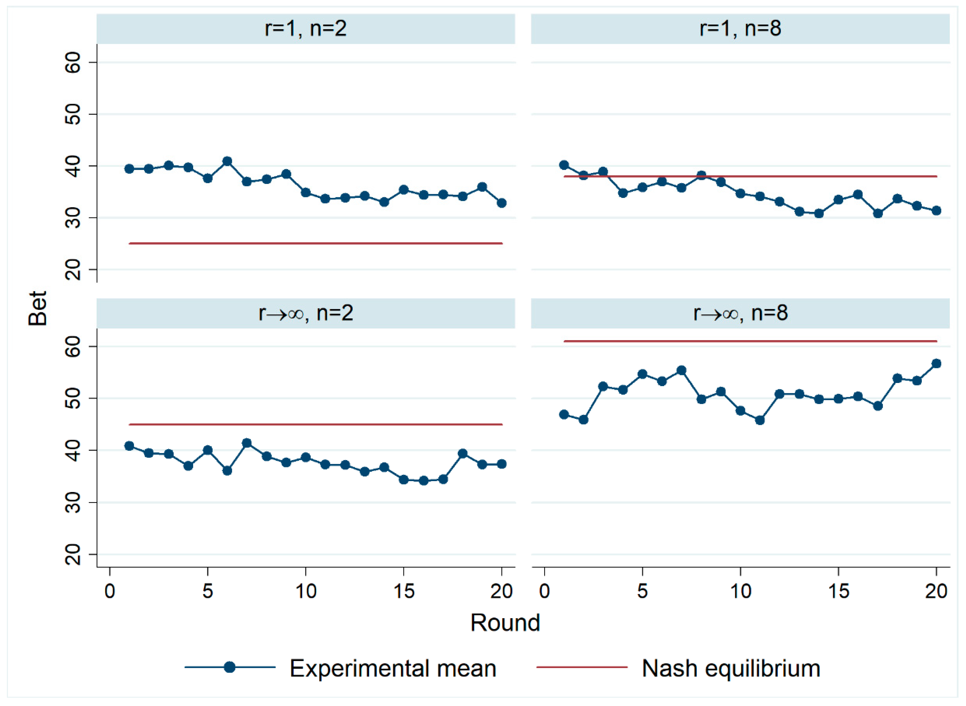
15
At the same time, it can be seen that risk-taking levels increase in the final three rounds in both treatments with r → ∞. This could hint at an end-effect during which collusion breaks down. So, even though from a theoretical perspective collusion should be more difficult to support with r → ∞ than with r = 1, we cannot rule out that some groups manage to attain at least some degree of tacit collusion which then breaks down near the end of the experiment.
16
The CH model assumes that there is distribution of player types with varying levels of cognition. Level-0 types have the lowest level of cognition and are assumed to pick a strategy at random. Level-1 types believe that other players are level-0 and choose a best response to that belief. Level-2 types believe that others players consist of a mixture level-0 and level-1 types and best respond to that belief. Generally, level-k types believe that other players are a mixture of lower types. The CH is then closed by assuming a specific distribution of types, usually a Poison distribution. For our implementation we have used a Poison distribution with parameter τ = 1.5 but the model predictions are quite robust to assuming other values of τ. Details are available from the authors upon request.
17
Note that in our experiment, subjects did not receive feedback on the choices of the other player(s). Hence, learning dynamics based on such information, such as best response learning or fictitious play, are not applicable.
18
The estimates are very similar if we use only the early rounds of the experiments.
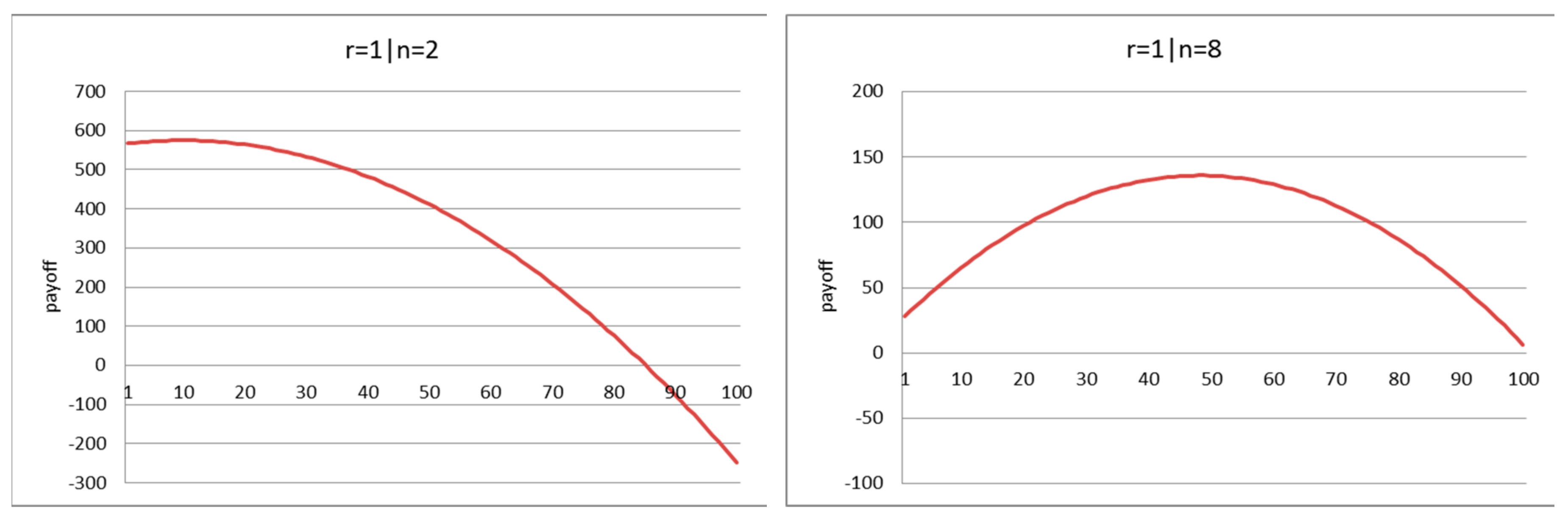
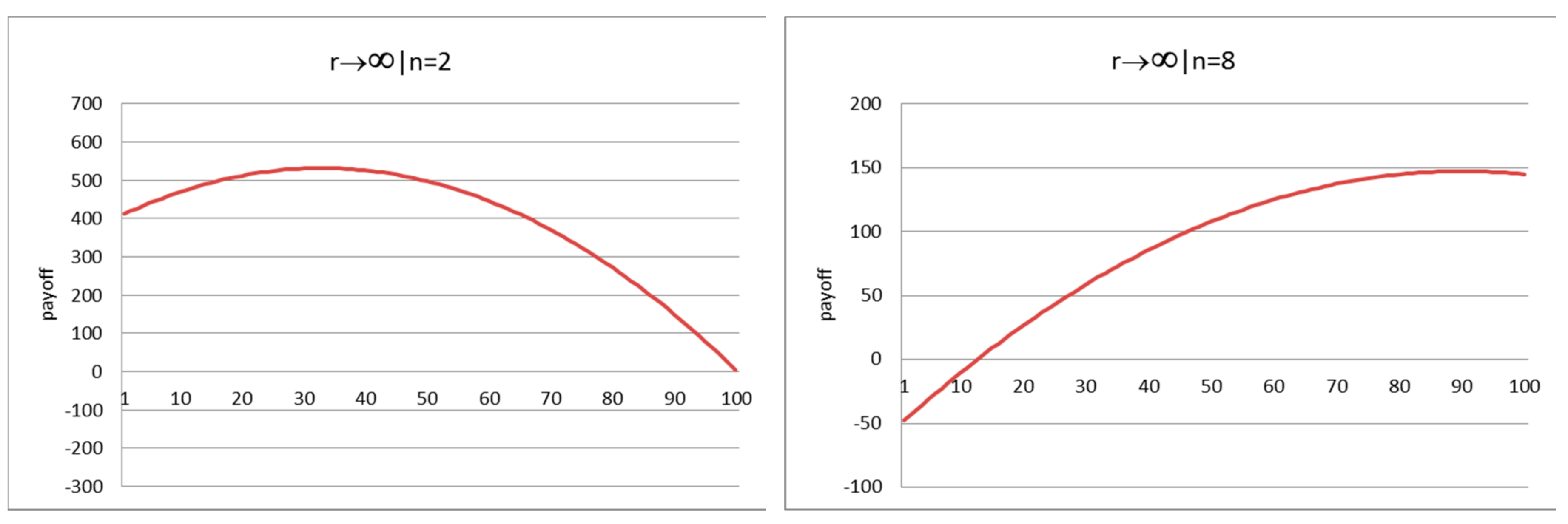
19
Note that these maxima do not necessarily coincide with Nash equilibrium. Still, of course, there is a relationship as both equilibrium and realized payoffs are based on the same payoff structure.
Figure 1. Development of average bets over the rounds.
Games 09 00072 g001
Figure 2. Empirical relationship between payoffs and bets.
Games 09 00072 g002aGames 09 00072 g002b
Table 1. Expected levels of risk taking in the Nash equilibrium.
nr = 1r → ∞
20.250.449
30.310.509
40.340.545
50.360.566
60.370.586
70.380.600
80.380.610
90.390.619
100.390.625
Notes: The value of the prize is v = 1, the cost of a crash is c = 0.05. For r → ∞, we present the expected (average) level of risk taking in the corresponding mixed strategies Nash equilibrium (MSNE).6
Table 2. Average bets by treatment.
TreatmentnM-W TestRow Total
28
r136.33 (8.07) [22]34.76 (5.08) [6]p = 0.95636.00 (7.48) [28]
37.68 (8.90) [19]50.97 (5.63) [6]p = 0.00640.87 (9.98) [25]
M-W testp = 0.583p = 0.004 p = 0.069
Column Total36.96 (8.38) [41]42.86 (9.89) [12]p = 0.04438.29 (9.00) [53]
Notes: Bets are averaged over all players and all rounds in a group. Standard deviations across groups are in parentheses. Numbers of observations (groups) are in brackets. p-values refer to Mann–Whitney U tests of the hypothesis that average bets in one treatment do not differ from average bets in the other treatment. See Appendix C for the corresponding power analyses of these tests. All numbers in square brackets represent numbers of observations.
Table 3. Regression of average bets in treatments and round.
Indep. Variable(1)(2)(3)(4)
r → ∞4.7251.3471.3471.347
(2.303) **(2.631)(2.633)(2.634)
n = 85.736−1.568−1.568−1.568
(2.575) **(2.561)(2.562)(2.564)
r → ∞ × n = 8 14.85514.8510.27
(3.886) ***(3.888) ***(4.301) **
round −0.252−0.301
(0.110) **(0.122) **
round × r → ∞ × n = 8 0.436
(0.175) **
cons34.7736.3338.9839.49
(1.632) ***(1.700) ***(2.164) ***(2.243) ***
R20.0800.1460.1610.165
number of observations1060106010601060
Notes: Ordinary Least Squares (OLS) regression with average bets per group per round as dependent variable. Robust standard errors are reported in parenthesis. Significance of coefficients indicated by ** p < 0.05; *** p < 0.01.
Table 4. Panel regressions of the bets per round and per subject.
Indep. Variable(1)(2)(3)
r → ∞1.3472.7272.631
(2.830)(2.701)(2.701)
n = 8−1.568−1.173−1.091
(2.641)(2.605)(2.608)
r → ∞ × n = 814.8613.13513.276
(4.046) ***(3.923) ***(3.92) ***
round−0.202−0.202−0.197
(0.093) **(0.093) **(0.095) *
female −1.092−0.972
(1.954)(0.196)
age −0.317−0.335
(0.286)(0.281)
find game complex 0. 6380.592
(0.361) *(0.363) *
prone to take risk 1.5111.491
(0.45) ***(0.453) ***
L.redchip 2.298
(0.767) **
L.win 0.575
(0.75)
cons38.4536.8536.113
(1.832) ***(7.65) ***(7.608) ***
R2 (overall)0.1080.1440.165
number of observations356035603382
number of subjects178178178
Notes: linear panel regressions with bet per subject per round as dependent variable. Robust standard errors are reported in parenthesis. Significance of coefficients indicated by * p < 0.1; ** p < 0.05; *** p < 0.01.

