Abstract
Small changes to the parameters of a system can lead to abrupt qualitative changes of its behavior, a phenomenon known as bifurcation. Such instabilities are typically considered problematic, however, we show that their power can be leveraged to design novel types of mechanisms. Hysteresis mechanisms use transient changes of system parameters to induce a permanent improvement to its performance via optimal equilibrium selection. Optimal control mechanisms induce convergence to states whose performance is better than even the best equilibrium. We apply these mechanisms in two different settings that illustrate the versatility of bifurcation mechanism design. In the first one we explore how introducing flat taxation could improve social welfare, despite decreasing agent “rationality,” by destabilizing inefficient equilibria. From there we move on to consider a well known game of tumor metabolism and use our approach to derive potential new cancer treatment strategies.
1. Introduction
The term bifurcation, which means splitting in two, is used to describe abrupt qualitative changes in system behavior due to smooth variation of its parameters. Bifurcations are ubiquitous and permeate all natural phenomena. Effectively, they produce discrete events (e.g., rain breaking out) out of smoothly varying, continuous systems (e.g., small changes to humidity or temperature). Typically, they are studied through bifurcation diagrams, multi-valued maps that prescribe how each parameter configuration translates to possible system behaviors (e.g., Figure 1).
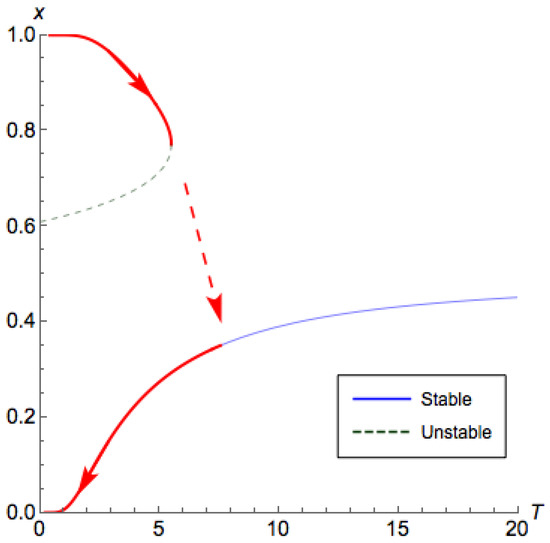
Figure 1.
Bifurcation diagram for a population coordination game. The x axis corresponds to the system temperature T, whereas the y axis corresponds to the projection of the proportion of the first population using the first strategy at equilibrium. For small T, the system exhibits multiple equilibria. Starting at , and by increasing the temperature beyond the critical threshold , and then bringing it back to zero, we can force the system to converge to another equilibrium.
Bifurcations arise in a natural way in game theory. Games are typically studied through their Nash correspondences, a multi-valued map connecting the parameters of the game (i.e., payoff matrices) to system behavior, in this case Nash equilibria. As we slowly vary the parameters of the game, typically the Nash equilibria will also vary smoothly, except at bifurcation points where, for example, the number of equilibria abruptly changes as some equilibria appear/disappear altogether. Such singularities may substantially impact both system behavior and system performance. For example, if the system state was at an equilibrium that disappeared during the bifurcation, then a turbulent transitionary period ensues where the system tries to reorganize itself at one of the remaining equilibria. Moreover, the quality of all remaining equilibria may be significantly worse than the original. Even more disturbingly, it is not a priori clear that the system will equilibrate at all. Successive bifurcations that lead to increasingly more complicated recurrent behavior is a standard route to chaos [1], which may have devastating effects on system performance.
Game theorists are particularly aware of the need to produce “robust" predictions, i.e., predictions that allow for deviations from an idealized exact specification of the parameters of the setting [2]. For example, -approximate Nash equilibria allow for the possibility of computational bounded agents, whereas -regret outcomes allow for persistently non-equilibrating behavior [3]. These approaches, however, do not really address the problem at its core as any solution concept defines a map from parameter space to behavioral space and no such map is immune to bifurcations. If pushed hard enough any system will destabilize. The question is what happens next?
Well, a lot of things may happen. It is intuitively clear that if we are allowed to play around arbitrarily with the payoffs of the agents then we can reproduce any game and no meaningful analysis is possible. Using payoff entries as controlling parameters is problematic for another reason. It is not clear that there exists a compelling parametrization of the payoff space that captures how real life decision-makers deviate from the Platonic ideal of the payoff matrix. Instead, we focus on another popular aspect of economic theory: agent “rationality”.
We adopt a standard model of boundedly rational learning agents. Boltzmann Q-learning dynamics [4,5,6] is a well studied behavioral model in which agents are parameterized by a temperature/rationality term T. Each agent keeps track of the collective past performance of his/her actions (i.e., learns from experience) and chooses an action according to a Boltzmann/Gibbs distribution with parameter T. When applied to a multi-agent game, the behavioral fixed points of Q-learning are known as quantal response equilibria (QREs) [7]. Naturally, QREs depend on the temperature T. As players become perfectly rational, and play approaches a Nash equilibrium,1 whereas as all agents use uniformly random strategies. As we vary the temperature the QRE(T) correspondence moves between these two extremes producing bifurcations along the way at critical points where the number of QREs changes (Figure 1).
Our goal in this paper is to quantify the effects of these rationality-driven bifurcations to the social welfare of two-player two-strategy games. At this point, a moment of pause is warranted. Why is this a worthy goal? Games of small size ( games in particular) are rarely seem like a subject worthy of serious scientific investigation. This, however, could not be further from the truth.
First, the correct way to interpret this setting is from the point of population games where each agent is better understood as a large homogeneous population (e.g., men and women, attackers and defenders, cells of phenotype A, and cells of phenotype B). Each of a handful of different types of users has only a few meaningful actions available to them. In fact, from the perspective of applied game theory, only such games with a small number of parameters are practically meaningful. The reason should be clear by now. Any game theoretic modeling of a real life scenario is invariably noisy and inaccurate. In order for game-theoretic predictions to be practically binding, they have to be robust to these uncertainties. If the system intrinsically has a large number of independent parameters, e.g., 20, then this parameter space will almost certainly encode a vast number of bifurcations, which invalidate any theoretical prediction. Practically useful models need to be small.
Secondly, game theoretic models applied for scientific purposes are often small. Specifically, the exact setting studied here with Boltzmann Q-learning dynamics applied in games has been used to model the effects of taxation to agent rationality [9] (see Section 6.2 for a more extensive discussion) as well as to model the effects of treatments that trigger phase transitions to cancer dynamics [10] (see Section 6.1). Our approach yields insights to explicit open questions in both of these applications areas. In fact, direct application of our analysis can address similar inquiries for any other phenomenon modeled by Q-learning dynamics applied in games.
Finally, the analysis itself is far from straightforward as it requires combining sets of tools and techniques that have so far been developed in isolation from each other. On one hand, we need to understand the behavior of these dynamical systems using tools from topology of dynamical systems, whose implications are largely qualitative (e.g., prove the lack of cyclic trajectories). On the other hand, we need to leverage these tools to quantify at which exact parameter values bifurcations occur and produce price-of-anarchy guarantees, which by definition are quantitative. As far as we know, this is the first instance of a fruitful combination of these tools. In fact, not only do we show how to analyze the effects of bifurcations to system efficiency, we also show how to leverage this understanding (e.g., knowledge of the geometry of the bifurcation diagrams) to design novel types of mechanisms with good performance guarantees.
Our Contribution
We introduce two different types of mechanisms: hysteresis and optimal control mechanisms.
Hysteresis mechanisms use transient changes to the system parameters to induce permanent improvements to its performance via optimal (Nash) equilibrium selection. The term hysteresis is derived from an ancient Greek word that means “to lag behind.” It reflects a time-based dependence between the system’s present output and its past inputs. For example, let’s assume that we start from a game theoretic system of Q-learning agents with temperature and assume that the system has converged to an equilibrium. By increasing the temperature beyond some critical threshold and then bringing it back to zero, we can force the system to provably converge to another equilibrium, e.g., the best (Nash) equilibrium (Figure 1, Theorem 4). Thus, we can ensure performance equivalent to that of the price of stability instead of the price of anarchy. One attractive feature of this mechanism is that from the perspective of the central designer it is relatively “cheap" to implement. Whereas typical mechanisms require the designer to continuously intervene (e.g., by paying the agents) to offset their greedy tendencies, this mechanism is transient with a finite amount of total effort from the perspective of the designer. Further, the idea that game theoretic systems have effectively systemic memory is rather interesting and could find other applications within algorithmic game theory.
Optimal control mechanisms induce convergence to states whose performance is better than even the best Nash equilibrium. Thus, we can at times even beat the price of stability (Theorem 5). Specifically, we show that by controlling the exploration/exploitation tradeoff, we can achieve strictly better states than those achievable by perfectly rational agents. In order to implement such a mechanism, it does not suffice to identify the right set of agents’ parameters/temperatures so that the system has some QRE whose social welfare is better than the best Nash. We need to design a trajectory through the parameter space so that this optimal QRE becomes the final resting point.
2. Preliminaries
2.1. Game Theory Basics: Games
In this paper, we focus on games. We define it as a game with two players, and each player has two actions. We write the payoff matrices of the game for each player as
respectively. The entry denotes the payoff for Player 1 when s/he chooses action i and his/her opponent chooses action j; similarly, denotes the payoff for Player 2 when s/he chooses action i and his/her opponent chooses action j. We define x as the probability that the Player 1 chooses his/her first action, and y as the probability that Player 2 chooses his/her first action. We also define two row vectors and as the strategy for each player. For simplicity, we denote the i-th entry of vector by . We call the tuple as the system state or the strategy profile.
An important solution concept in game theory is the Nash equilibrium, where each user cannot make profit by unilaterally changing his/her strategy, that is
Definition 1 (Nash equilibrium).
A strategy profile is a Nash equilibrium (NE) if
We call a pure Nash equilibrium (PNE) if both and . A Nash equilibrium assumes each user is fully rational. An alternative solution concept is the quantal response equilibrium [7], where it assumes that each user has bounded rationality:
Definition 2 (Quantal response equilibrium).
A strategy profile is a QRE with respect to temperature and if
Analogous to the definition of Nash equilibria, we can consider the QREs as the case where each player is not only maximizing the expected utility but also maximizing the entropy. We can see that the QREs are the solutions to maximizing the linear combination of the following program:
This formulation has been widely seen in Q-learning dynamics literature (e.g., [9,11,12]). With this formulation, we can find that the two parameters and control the weighting between the utility and the entropy. We call and the temperatures, and their values define the level of irrationality. If and are zero, then both players are fully rational, and the system state is a Nash equilibrium. However, if both and are infinity, then each player is choosing his/her action according to a uniform distribution, which corresponds to the fully irrational players.
2.2. Efficiency of an Equilibrium
The performance of a system state can be measured via the social welfare. Given a system state , we define the social welfare as the sum of the expected payoff of all users in the system:
Definition 3.
Given a game with payoff matrices and , and a system state , the social welfare is defined as
In the context of algorithmic game theory, we can measure the efficiency of a game by comparing the best social welfare with the social welfare of equilibrium system states. We call the strategy profile that achieves the maximal social welfare as the socially optimal (SO) strategy profile. The efficiency of a game is often described as the notion of the price of anarchy (PoA) and the price of stability (PoS). Given a set of equilibrium states S, we define the PoA/PoS as the ratio of the social welfare of the socially optimal state to the social welfare of the worst/best equilibrium state in S, respectively. Formally,
Definition 4.
Given a game with payoff matrices A and B, and a set of equilibrium system states , the price of anarchy (PoA) and the price of stability (PoS) are defined as
3. Our Model
3.1. Q-Learning Dynamics
In this paper, we are particularly interested in the scenario when both players’ strategies are evolving under Q-learning dynamics:
Q-learning dynamics has been studied because of its connection with multi-agent learning problems. For example, it has been shown in [13,14] that Q-learning dynamics captures the system evolution of a repeated game, where each player learns his/her strategy through Q-learning and Boltzmann selection rules. More details are provided in Appendix A.
An important observation on the dynamics of Equation (2) is that it demonstrates the exploration/exploitation tradeoff [14]. We can find that the right hand side of Equation (2) is composed of two parts. The first part is exactly the vector field of replicator dynamic [15]. Basically, the replicator dynamics drives the system to the state of higher utility for both players. As a result, we can consider this as a selection process in terms of population evolutionary, or an exploitation process from the perspective of a learning agent. Then, for the second part, we show in the appendix that if the time derivative of contains this part alone, this results in an increase of the system entropy.
The system entropy is a function that captures the randomness of the system. From the population evolutionary perspective, the system entropy corresponds to the variety of the population. As a result, this term can be considered as the mutation process. The level of the mutation is controlled by the temperature parameters and . Besides, in terms of the reinforcement learning, this term can be considered as an exploration process, as it provides the opportunity for the agent to gain information about the action that does not look the best so far.
3.2. Convergence of the Q-Learning Dynamics
By observing the Q-learning dynamics of Equation (2), we can find that the interior rest points for the dynamics are exactly the QREs of the game. It is claimed in [16] (albeit without proof) that the Q-learning dynamics for a game converges to interior rest points of probability simplexes for any positive temperature and . We provide a formal proof in Appendix B. The idea is that, for positive temperatures, the system is dissipative and, by leveraging the planar nature of the system, it can be argued that it converges to fixed points.
3.3. Rescaling the Payoff Matrix
At the end of this section, we discuss the transformation of the payoff matrices that preserves the dynamics in Equation (2). This idea is proposed in [17,18], where the rescaling of a matrix is defined as follows
Definition 5
([18]). and is said to be a rescaling of and if there exist constants , and , such that and .
It is clear that rescaling the game payoff matrices is equivalent to updating the temperature parameters of the two agents in Equation (2). Therefore, it suffices to study the dynamics under the assumption that the payoff matrices and are in the following diagonal form.
Definition 6.
Given matrices and , their diagonal form is defined as
Note that, although rescaling the payoff matrices to their diagonal form preserves the equilibria, it does not preserve the social optimality, i.e., the socially optimal strategy profile in the transformed game is not necessarily the socially optimal strategy profile in the original game.
4. Hysteresis Effect and Bifurcation Analysis
4.1. Hysteresis effect in Q-Learning Dynamics: An Example
We begin our discussion with an example:
Example 1 (Hysteresis effect).
Consider a game with reward matrices
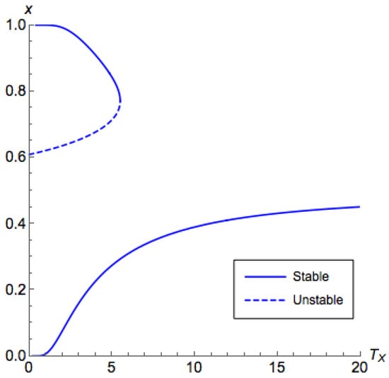
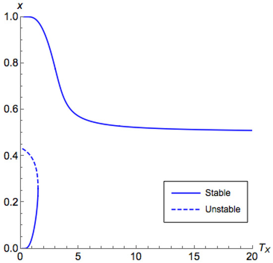
There are two PNEs in this game: and . By fixing different , we can plot different QREs with respect to as in Figure 2 and Figure 3, which we call the bifurcation diagrams. For simplicity, we only show the value of x in the figure, since, according to Equation (4), given x and , the value of y can be uniquely determined. Assuming the system follows the Q-learning dynamics, as we slowly vary , x tends to stay on the line segment that is the closest to where it was originally corresponding to a stable but inefficient fixed point. We consider the following process:

Figure 2.
The bifurcation diagram for Example 1 with . The horizontal axis corresponds to the temperature for the first (row) player and the vertical axis corresponds to the probability that the first player chooses the first action in equilibrium. There exist three branches (two stable and one unstable). For , there are two branches appearing in pairs, and they occur only when is less than some value. For , there is a branch, which we call the principal branch, where the quantal response equilibrium (QRE) always exists for any .

Figure 3.
Bifurcation diagram for Example 1 with . The horizontal axis corresponds to the temperature for the first (row) player and the vertical axis corresponds to the probability that the first player chooses the first action in equilibrium. Similar to Figure 2, there exist three branches (two stable and one unstable). However, unlike Figure 2, now the two branches appearing in pairs happen at , and the principal branch is at .
- 1.
- Where the initial state is , where and , plot x versus by fixing in Figure 3.
- 2.
- Fix and increase to where there is only one QRE correspondence.
- 3.
- Fix and decrease back to 1. Now .
In the above example, we can find that, although at the end the temperature parameters are set back to their initial value, the system state ends up being an entirely different equilibrium. This behavior is known as the hysteresis effect. In this section, we would like to answer the question of when this is going to happen. Further, in the next section, we will show how can we take advantage of this phenomenon.
4.2. Characterizing QREs
We consider the bifurcation diagrams for QREs in games. Without loss of generality, we consider a properly rescaled game with payoff matrices in the diagonal form:
We can also assume that the action indices are ordered properly and rescaled properly so that and . For simplicity, we assume and do not hold at the same time. At QRE, we have
Given and , there could be multiple solutions to Equation (4). However, we find that, if we know the equilibrium states, then we can recover the temperature parameters. We solve for and in Equation (4) and get
We call this the first form of representation, where and are written as functions of x and y. Here the capital subscripts for and indicate that they are considered as functions. A direct observation of Equation (5) is that both of them are continuous function over except for and .
An alternative way to describe the QRE is to write and y as a function of x and parameterize with respect to in the following second form of representation. This will be the form that we use to prove many useful characteristics of QREs.
In this way, if we are given , we are able to analyze how changes with x. This helps us understand how to answer the question of what the QREs are given and in the system.
We also want to analyze the stability of the QREs. From dynamical system theory (e.g., [19]), a fixed point of a dynamical system is said to be asymptotically stable if all of the eigenvalues of its Jacobian matrix have a negative real part; if it has at least one eigenvalue with a positive real part, then it is unstable. It turns out that, under the second form representation, we are able to determine whether a segment in the diagram is stable or not.
Lemma 1.
Given , the system state is a stable equilibrium if and only if
- 1.
- if ;
- 2.
- if .
Proof.
The given condition is equivalent to the case where both eigenvalues of the Jacobian matrix of the dynamics (2) are negative. ☐
Finally, we define the principal branch. In Example 1, we call the branch on the principal branch given , since, for any , there is some such that . Analogously, we can define it formally as in the following definition with the help of the second form representation.
Definition 7.
Given , the region contains the principal branch of QRE correspondence if it satisfies the following conditions:
- 1.
- is continuous and differentiable for .
- 2.
- for .
- 3.
- For any , there exists such that .
Further, for a region that contains the principal branch, is on the principal branch if it satisfies the following conditions:
- 1.
- The equilibrium state is stable.
- 2.
- There is no such that .
4.3. Coordination Games
We begin our analysis with the class of coordination games, where we have all , , , and positive. Additionally, without loss of generality, we assume . In this case, there is no dominant strategy for either player, and there are two PNEs.
- Given , there are three branches. One is the principal branch, while the other two appear in pairs and occur only when is less than some value.
- For small , the principal branch goes toward ; for a large , the principal branch goes toward .
Now, we are going to show that these observations are generally true in coordination games. The proofs in this section are deferred to Appendix D, where we will provide a detailed discussion on the proving techniques.
The first idea we are going to introduce is the inverting temperature, which is the threshold of in Observation (2). We define it as
We note that is positive only if , which is the case where two players have different preferences. When , as the first player increases his/her rationality from fully irrational, i.e., decreases from infinity, s/he is likely to be influenced by the second player’s preference. If is greater than , then the first player prefers to follow his/her own preference, making the principal branch move toward . We formalize this idea in the following theorem:
Theorem 1 (Direction of the principal branch).
Given a coordination game, and given , the following statements are true:
- 1.
- If , then contains the principal branch.
- 2.
- If , then contains the principal branch.
The second idea is the critical temperature, denoted as , which is a function of . The critical temperature is defined as the infimum of such that, for any , there is a unique QRE correspondence under . Generally, there is no close form for the critical temperature. However, we can still compute it efficiently, as we show in Theorem 2. Another interesting value of we should point out is , which is the maximum value of that QREs not on the principal branch are presenting. Intuitively, as goes beyond , the first player ignores the decision of the second player and turns his/her face to what s/he thinks is better. We formalize the idea of and in the following theorem:
Theorem 2 (Properties about the second QRE).
Given a coordination game, and given , the following statements are true:
- 1.
- For almost every , all QREs not lying on the principal branch appear in pairs.
- 2.
- If , then there is no QRE correspondence in .
- 3.
- If , then there is no QRE correspondence for in .
- 4.
- If , then there is no QRE correspondence for in .
- 5.
- is given as , where is the solution to the equality
- 6.
- can be found using binary search.
The next aspect of the QRE correspondence is their stability. According to Lemma 1, the stability of the QREs can also be inspected with the advantage of the second form representation by analyzing . We state the results in the following theorem:
Theorem 3 (Stability).
Given a coordination game, and given , the following statements are true:
- 1.
- If , then the principal branch is continuous.
- 2.
- If , then the principal branch is continuous.
- 3.
- If and , then the principal branch may not be continuous.
- 4.
- If is fixed, for the pairs of QREs not lying on the principal branch, the one with the lowest distance to is unstable, while the other one is stable.
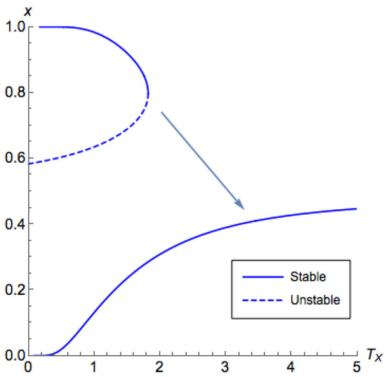
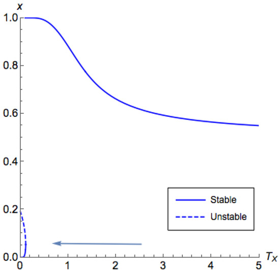
Note that Part 3 in Theorem 3 infers that there is potentially an unstable segment between segments of the principal branch. This phenomenon is illustrated in Figure 4 and Figure 5. Though this case is weaker than other cases, this does not hinder us from designing a controlling mechanism as we are going to do in Section 5.3.
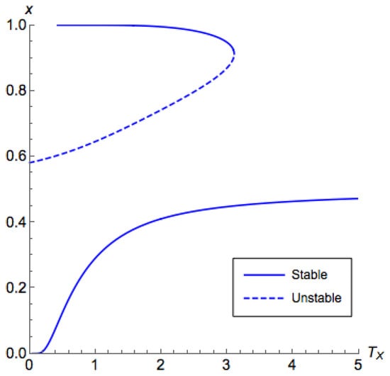
Figure 4.
Bifurcation diagram for a coordination game with and a low . The horizontal axis corresponds to the temperature for the first (row) player and the vertical axis corresponds to the probability that the first player chooses the first action in equilibrium. We can find that the principal branch is contained in .
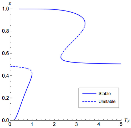
Figure 5.
Bifurcation diagram for a coordination game with and a high . The horizontal axis corresponds to the temperature for the first (row) player and the vertical axis corresponds to the probability that the first player chooses the first action in equilibrium. We can find that the principal branch is contained in . In addition, there is a non-stable segment on the principal branch.
4.4. Non-Coordination Games
Due to space constraints, the analysis for non-coordination games is deferred to Appendix C.
5. Mechanism Design
In this section, we aim to design a systematic way to improve the social welfare in a game by changing the temperature parameters. We focus our discussion on the class of coordination games. Recall that any game has more than one PNE if and only if its diagonal form is a coordination game. This means that, in a coordination game, given any temperature parameters, there could be more than one equilibrium correspondences. In this case, we are not guaranteed to achieve the socially optimal equilibrium state even if we set the system to the correct temperatures due to the hysteresis effects that we have discussed in the previous section. Therefore, the main task for us in this section is to determine when and how we can get to the socially optimal equilibrium state. In Section 5.3, we consider the case when the socially optimal state is one of the PNEs. Since rescaling the payoff matrices to their diagonal form does not preserve the social optimality, in Section 5.1, we generalize our discussion to the case when the social optimal state does not coincide with any PNE.
5.1. Hysteresis Mechanism: Select the Best Nash Equilibrium via QRE Dynamics
First, we consider the case when the socially optimal state is one of the PNEs. The main task for us in this case is to determine when and how we can get to the socially optimal PNE. In Example 1, by sequentially changing , we move the equilibrium state from around to around , which is the social optimum state. We formalize this idea as the hysteresis mechanism and present it in Theorem 4. The hysteresis mechanism mainly takes advantage of the hysteresis effect we have discussed in Section 4—that we use transient changes of system parameters to induce permanent improvements to system performance via optimal equilibrium selection.
Theorem 4 (Hysteresis Mechanism).
Consider a game that satisfies the following properties:
- 1.
- Its diagonal form satisfies .
- 2.
- Exactly one of its pure Nash equilibrium is the socially optimal state.
Without loss of generality, we can assume . Then there is a mechanism to control the system to the social optimum by sequentially changing and if (1) and (2) the socially optimal state is do not hold at the same time.
Proof.
First, note that, if , by Theorem 1, the principal branch is always in the region . As a result, once is increased beyond the critical temperature, the system state will no longer return to at any positive temperature. Therefore, cannot be approached from any state in through the QRE dynamics.
On the other hand, if and the socially optimal state is the PNE , then we can approach that state by first getting onto the principal branch. The mechanism can be described as
| (C1) | (a) | Raise to some value above the critical temperature . |
| (b) | Reduce and to 0. |
Though in this case the initial choice of does not affect the result, if the social designer is taking the costs from assigning large and values into account, s/he is going to trade off between and since a typically smaller induces a larger .
Next, consider . If we are aiming for state , then we can undergo the following procedure:
| (D1) | (a) | Keep at some value below . Now the principal branch is at . |
| (b) | Raise to some value above the critical temperature . | |
| (c) | Reduce to 0. | |
| (d) | Reduce to 0. |
On the other hand, if we are aiming for state , then the following procedure suffices:
| (D2) | (a) | Keep at some value above . Now the principal branch is at . |
| (b) | Raise to some value above the critical temperature . | |
| (c) | Reduce to 0. | |
| (d) | Reduce to 0. |
Note that, in the last two steps, only by reducing after keeps the state around . We recommend that the interested reader refers to Figure 11 for Case (D1) and Figure 12 for Case (D2) for more insights. ☐
5.2. Efficiency of QREs: An Example
A question that arises with the solution concept of QRE is whether QRE improves social welfare? Here we show that the answer is yes. We begin with an example to illustrate:
Example 2.
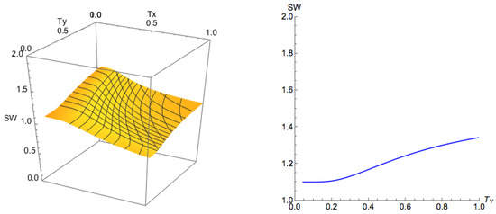
Consider a standard coordination game with the payoff matrices of the form
where are some small numbers. Note that, in this game, there are two PNEs, and , with social welfare values and , respectively. We can see that for small ϵ and values, the socially optimal state is , with social welfare value 2. In this case, the state is the PNE with the best social welfare. However, we are able to achieve a state with better social welfare than any NE through QRE dynamics. We illustrate the social welfare of the QREs with different temperatures of this example in Figure 6. In this figure, we can see that, at PNE, which is the point , the social welfare is . However, we are able to increase the social welfare by increasing . We will show in Section 5.3 a general algorithm for finding particular temperature as well as a mechanism, which we refer to as the optimal control mechanism, that drives the system to the desired state.

Figure 6.
The left figure is the social welfare on the principal branch for Example 2, and the right figure is an illustration when . We can see that by increasing , we can obtain an equilibrium with a social welfare higher than that of the best Nash equilibrium (which is ).
5.3. Optimal Control Mechanism: Better Equilibrium with Irrationality
Here, we show a general approach to improve the PoS bound for coordination games from Nash equilibria by QREs and Q-learning dynamics. We denote as the set of QREs with respect to and . Further, denote as the set of the union of over all positive and . Additionally, denote the set of pure Nash equilibria system states as . Since the set is the limit of as and approach zero, we have the bounds:
Then, we define QRE-achievable states:
Definition 8.
A state is a QRE-achievable state if for every , there is a positive finite and and such that and .
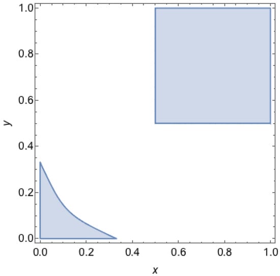
Note that, with this definition, pure Nash equilibria are QRE-achievable states. However, the socially optimal states are not necessarily QRE-achievable. For example, we illustrate in Figure 7 the set of QRE-achievable states for Example 2. We can find that the socially optimal state, , is not QRE-achievable. Nevertheless, it is easy to see from Figure 7 and Figure 8 that we can achieve a higher social welfare at , which is a QRE-achievable state. Formally, we can describe the set of QRE-achievable states as the positive support of and :
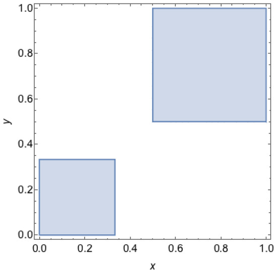
Figure 7.
Set of QRE-achievable states for Example 2. A point represents a mixed strategy profile where the first agent chooses its first strategy with probability x and the second agent chooses its first strategy with probability y. The grey areas depict the set of mixed strategy profiles that can be reproduced as QRE states for Example 2, i.e., these are outcomes for which there are temperature parameters for which the mixed strategy profile is a QRE.
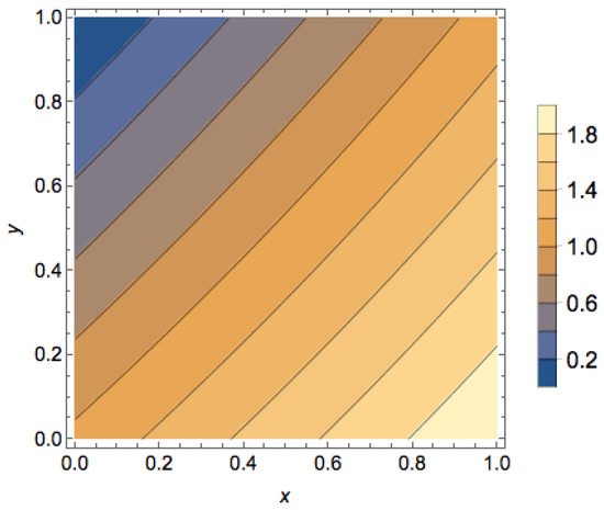
Figure 8.
Social welfare for all states in Example 2. A point represents a mixed strategy profile where the first agent chooses its first strategy with probability x and the second agent chooses its first strategy with probability y. The color of the point corresponds to the social welfare of that mixed strategy profile with states of higher social welfare corresponding to lighter shades. The optimal state is , whereas the worst state is .
An example for the region of a game with is illustrated in Figure 7. For the case , we demonstrate it in Figure 9.
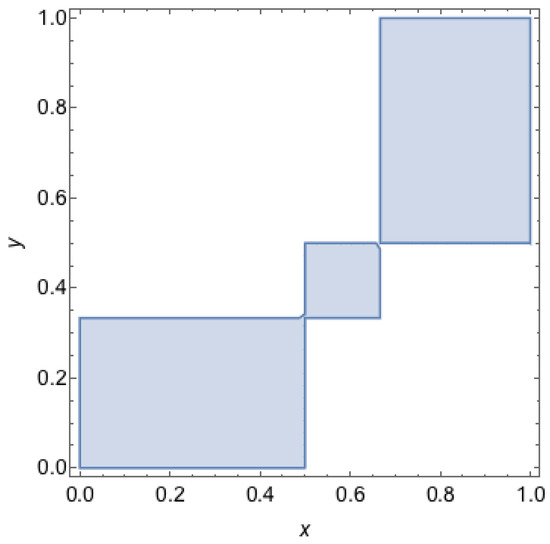
Figure 9.
Set of QRE-achievable states for a coordination game with . A point represents a mixed strategy profile where the first agent chooses its first strategy with probability x and the second agent chooses its first strategy with probability y. The grey areas depict the set of mixed strategy profiles that can be reproduced as QRE states a coordination game with , i.e., these are outcomes for which there exists temperature parameters for which the mixed strategy profile is a QRE.
In the following theorem, we propose the optimal control mechanism for a general process to achieve an equilibrium that is better than the PoS bound from Nash equilibria.
Theorem 5 (Optimal Control Mechanism).
Given a game, if it satisfies the following property:
- 1.
- Its diagonal form satisfies .
- 2.
- None of its pure Nash equilibrium is the socially optimal state.
Without loss of generality, we can assume . Then
- 1.
- there is a stable QRE-achievable state whose social welfare is better than any Nash equilibrium;
- 2.
- there is a mechanism to control the system to this state from the best Nash equilibrium by sequentially changing and .
Proof.
Note that, given those properties, there are two PNEs and . Since we know neither of them is socially optimal, the socially optimal state must be either or .
First, consider . In this case, we know from Theorem 3 that all states belong to a principal branch for some and are stable, while for not all of them are stable. We illustrate the region of stable QRE-achievable states in Figure 10. By Theorems 2 and 3, we can infer that the states near the border are stable. As a result, we can claim that the following states are what we are aiming for:

Figure 10.
Stable QRE-achievable states for a coordination game with . A point represents a mixed strategy profile, where the first agent chooses its first strategy with probability x and the second agent chooses its first strategy with probability y. The grey areas depict the set of mixed strategy profiles that can be reproduced as stable QRE states a coordination game with , i.e., these are outcomes for which there are temperature parameters for which the mixed strategy profile is a stable QRE.
- (A1)
- If is the best NE and is the SO state, then we select .
- (A2)
- If is the best NE and is the SO state, then we select .
- (A3)
- If is the best NE and is the SO state, then we select .
- (A4)
- If is the best NE and is the SO state, then we select .
It is clear that these choices of states improve the social welfare. It is known that for the class of games we are considering, the price of stability is no greater than 2. In fact, in Cases A1 and A2, we reduce this factor to . Additionally, in Cases A3 and A4, we reduce this factor to .
The next step is to show the mechanism to drive the system to the desired state. Due to symmetry, we only discuss Cases A1 and A3, where Cases A2 and A4 can be done analogously. For Case A1, the state corresponds to the temperatures and . For any small , we can always find the state on the principal branch of some . This means that we can achieve this state from any initial state, not only from the NEs. With the help of the first form representation of the QREs in Equation (5), given any QRE-achievable system state , we are able to recover them to corresponding temperatures through and . The mechanism can be described as follows:
| (A1) | (a) | From any initial state, raise to . |
| (b) | Decrease to . |
For Case A3, the state we selected is not on the principal branch. This means that we cannot increase the temperatures too much; otherwise, the system state will move to the principal branch and will never return. We assume initially the system state is at for some small , which is some state close to the best NE. Additionally, we can assume the initial temperatures are and . Our goal is to arrive at the state for some small and such that is stable. We present the mechanism in the following:
| (A3) | (a) | From the initial state , move to . |
| (b) | Increase to . |
Here, note that Step (b) should not proceed before Step (a) because, if we increase first, then we risk leaving the principal branch.
Next, consider the case where . Similarly to the previous case, we know from Theorems 2 and 3 that states near the borders and are basically stable states. Hence, we can claim the following results:
- (B1)
- If is the best NE and is the SO state, then we select .
- (B2)
- If is the best NE and is the SO state, then we select .
- (B3)
- If is the best NE and is the SO state, then we select .
- (B4)
- If is the best NE and is the SO state, then we select .
It is clear that these choices of states create improvement on the social welfare. An interesting result for this case is that basically these desired states can be reached from any initial state. Due to symmetry, we demonstrate the mechanisms for Cases (B3) and (B4), and the remaining ones can be done analogously.
For Case (B3), we are aiming for the state for some small and . We propose the following mechanism:
| (B3) | Phase 1: Getting to the principal branch.
|
Phase 2: Staying at the current branch.
|
This process is illustrated in Figure 11 and Figure 12. In Phase 1, as we are keeping low , meaning the second player is of more rationality. As the first player getting more rational, s/he is more likely to be influenced by the second player’s preference, and eventually getting to a Nash equilibrium. In phase 2, we make the second player more irrational to increase the social welfare. The level of irrationality we add in phase 2 should be capped to prevent the first player to deviate his/her decision.

Figure 11.
Illustration for Phase 1 in Case (B3), where we keep low but increase and then decrease back to a small value. In this phase, the equilibrium state moves from the branch where to the principal branch (the branch where ).

Figure 12.
Illustration for Phase 2 in Case (B3). In this phase, we increase to . The principal branch switches from to and the equilibrium state stays on the branch (the branch pointed out by the blue arrow) only if is low.
For Case (B4), since our desired state is on the principal branch, the mechanism will be similar to Case (A1).
☐
| (B4) | (a) | From any initial state, raise to . |
| (b) | Decrease to . |
As a remark, in Cases (A3) and (A4), if we do not start from but from some other states on the principal branch, we can instead aim for state . This state is not better than the best Nash equilibrium, but still makes improvements over the initial state. The process can be modified as
| (A3’) | (a) | From any initial state, raise to (above ). |
| (b) | Reduce to . |
6. Applications
6.1. Evolution of Metabolic Phenotypes in Cancer
Evolutionary game theory (EGT) has been instrumental in studying evolutionary aspects of the somatic evolution that characterizes cancer progression. As opposed to conventional game theory, in evolutionary game theory, the strategies are fixed for the player and constitute its phenotype. Tumors are very heterogeneous, and frequency-dependent selection is a driving force in somatic evolution. While evolutionary outcomes can change depending on initial conditions or on the exact features and microenvironment of the relevant tumor phenotypes, evolutionary game theory can explain why certain clonal populations, usually the more aggressive and faster proliferating ones, emerge and overtake the previous ones. Tomlinson and Bodmer were the first to explore the role of cell–cell interactions in cancer using EGT [20]. This pioneering work was followed by others that built on those initial ideas to study the role of key aspects of cancer evolution, such as the role of space [21] treatment [22,23] or metabolism [10,24].
Work by Kianercy and colleagues [10] shows how microenvironmental heterogeneity impacts somatic evolution. Kianercy and colleagues show how the tumor’s genetic instability adapts to the heterogeneous microenvironment (with regard to oxygen concentration) to better tune metabolism to the dynamic microenvironment. While evolutionary dynamics can help a tumor population evolve to acquire all relevant mutations to become an aggressive cancer [25], they also help them become treatment-resistant, which leads to treatment failure as well as increased toxicity for the patient, which can result in patient death. Researchers such as Axelrod and colleagues [26] have speculated that tumor cells do not need to acquire all the hallmarks of cancer to become an aggressive cancer but that the cooperation between different cells with different abilities might allow the tumor as a whole to acquire all the hallmarks. A few years ago, Hanahan and Weinberg updated their original research to include disregulated metabolisms as one of the hallmarks of cancer [27]. Here we suggest that cooperation between cells with different metabolic needs and abilities could allow the tumor to grow faster but also present a new therapeutical target that could be clinically exploited. Namely, this cooperation, as described by Kinaercy and colleagues, allows for hypoxic cells to benefit from the presence of oxygenated non-glycolytic cells with modest glucose requirements, whereas cells with aerobic metabolism can benefit from the lactic acids that are the byproduct of anaerobic metabolism (see Figure 13).
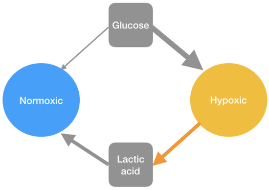
Figure 13.
Interaction diagram between different type of cells. The hypoxic cells can benefit from the presence of oxygenated non-glycolytic cells with modest glucose requirements, whereas cells with aerobic metabolism can benefit from the lactic acids that are the byproduct of anaerobic metabolism.
By targeting this cooperation, a tumor’s growth and progression could be disrupted using novel microenvironmental pH normalizers. What our work suggests is that small perturbations could return the system back to a state different from the one it started so that the microenvironmental impact does not need to be too substantial for the therapy to have an impact. The work we have described here supports the hypothesis that hysteresis would allow us to apply treatments for a short duration of time with the aim of changing the nature of the game instead of killing tumor cells. This would have the combined advantages of reducing toxicity and side effects and decreasing selection for resistant tumor phenotypes and thus reducing the emergence of resistance to the treatment. For instance, treatments that aim to reduce the acidity of the environment [28] would impact not only acid producing cells but also the acid-resistant normoxic ones.
Our techniques (the hysteresis mechanism and the optimal control mechanism) can be applied to the cancer game [10] with two types of tumor phenotypic strategies: hypoxic cells and oxygenated cells (Table 1). These cells inhabit regions where oxygen could be either abundant or lacking. In the former, oxygenated cells with regular metabolism thrive but in the latter, hypoxic cells whose metabolism is less reliant on the presence of oxygen (but more on the presence of glucose) have higher fitness.

Table 1.
Payoff matrix for the cancer game in [10], where . This game represents the tumor metabolic symbiosis rewards (ATP generation). The row agent represents hypoxic cells, and the column one represents oxygenated cell energy generation values based on their collective actions. Specifically, oxygenated cells can use both glucose and lactate for energy generation, whereas the hypoxic cells can use only glucose. Empirical data as discussed in [10] suggests that .
6.2. Taxation
A direct application for the solution concept of QRE is to analyze the effect of taxation, which has been discussed in [9]. Unlike Nash equilibria, for QREs, if we multiply the payoff matrix by some factor , the equilibrium does change. This is because, by multiplying , effectively we are dividing the temperature parameters by . This means that, if we charge taxes to the players with some flat tax rate , the QREs will differ. Formally, we define the base temperature as the temperature when no tax is applied for both players. Then, we can define the tax rate for each player as , respectively.
We demonstrate how the hysteresis mechanism can be applied in a game via taxation with Example 1. Recall that in Example 1, we have two types of agents. We can consider these two types of agents as corresponding to two different sectors of the economy (e.g., aircraft manufacturing versus car manufacturing), which need to coordinate on their choice between two different competing technologies that are related to both sectors (e.g., 3D-printing). We can consider the row player as being the aircraft manufacturer and the column player as being the car manufacturer, with payoff matrices specified in Table 2. By assuming both players are of bounded rationality with temperature 1, we assume the base temperatures for both players are . In this game, the equilibrium where both players choose Technology 1 has greater social welfare than the equilibrium where both players choose Technology 2. Consider the situation where, initially, the system is in an equilibrium state where both players choose Technology 2 with high probability. Then, with taxation, we have shown in the previous sections that we are able to increase the social welfare via the hysteresis mechanism or the optimal control mechanism. Here, we demonstrate how the simplified process that we have described in Example 1 can improve the social welfare in this game (see Figure 2 for the bifurcation diagram of this game):

Table 2.
Payoff matrix for a coordination game between two agents where neither of the two pure Nash Pareto dominates the other. States where both agents play the first strategy (Technology 1) are nearly socially optimal and they can be selected via a bifurcation argument.
- The initial state is , where the row agent chooses Technology 1 with probability and the column agent chooses Technology 1 with probability . This is an equilibrium state when we impose the tax rate to the row agent and the tax rate to the column agent (where and ).
- Fix the tax rate for the column agent at (where ) and increase the tax rate for the row agent to (where ). Under this assignment of tax rates, there is only one QRE correspondence.
- Fix the tax rate for the column agent at (where ) and decrease the tax rate for the row agent back to 0 (where ). Now , where both agents choose Action 1 with high probability.
In [9], they considered three approaches—“anarchy,” “socialism,” and “market”—of how the taxes can be dynamically adjusted by the society, depending on whether the taxes are determined in a decentralized manner, by an external regulator, or through bargaining, respectively. The concept of our mechanisms is a variant of the “socialism” scheme since in our model the mechanism, who can be thought as an external regulator, determines the tax rates. Our mechanisms are systematic approaches that optimize an objective where, in [9], the trajectories toward maximizing expected utilities are considered.
7. Connection to Previous Works
Recently, there has been a growing interplay between game theory, dynamical systems, and computer science. Examples include the integration of replicator dynamics and topological tools [29,30,31] in algorithmic game theory, and Q-learning dynamics [5] in multi-agent systems [6]. Q-learning dynamics has been studied extensively in game settings, e.g., by Sato et al. in [13] and Tuyls et al. in [14]. In [12], Q-learning dynamics is considered as an extension of replicator dynamics driven by a combination of payoffs and entropy. Recent advances in our understanding of evolutionary dynamics in multi-agent learning can be found in the survey in [32].
We are particularly interested in the connection between Q-learning dynamics and the concept of QRE [7] in game theory. In [11], Cominetti et al. study this connection in traffic congestion games. The hysteresis effect of Q-learning dynamics was first identified in 2012 by Wolpert et al. [9]. Kianercy et al. in [16] observed the same phenomenon and provided discussions on bifurcation diagrams in games. The hysteresis effect has also been highlighted in recent follow-up work by [10] as a design principle for future cancer treatments. It was also studied in [33] in the context of minimum-effort coordination games. However, our current understanding is still mostly qualitative and in this work we have pushed towards a more practically applicable, quantitative, and algorithmic analysis.
Analyzing the characteristics of various dynamical systems has also been attracting the attention of computer science community in recent years. For example, besides the Q-learning dynamics, the (simpler) replicator dynamics has been studied extensively due to its connections [30,34,35] to the multiplicative weight update (MWU) algorithm in [36].
Much attention has also been devoted to biological systems and their connections to game theory and computation. In recent work by Mehta et al. [37], the connection with genetic diversity was discussed in terms of the complexity of predicting whether genetic diversity persists in the long run under evolutionary pressures. This paper builds upon a rapid sequence of related results [38,39,40,41,42,43]. The key result is [39,40], where it was made clear that there is a strong connection between studying replicator dynamics in games and standard models of evolution. Follow-up works show how dynamics that incorporate errors (i.e., mutations) can be analyzed [44] and how such mutations can have a critical effect on ensuring survival in the presence of dynamically changing environments. Our paper makes progress along these lines by examining how noisy dynamics can introduce, for example, bifurcations.
We were inspired by recent work by Kianercy et al. establishing a connection between cancer dynamics and cancer treatment and studying Q-learning dynamics in games. This is analogous to the connections [39,40,45] between MWU and evolution detailed above. It is our hope that by starting off a quantitative analysis of these systems we can kickstart similarly rapid developments in our understanding of the related questions.
8. Conclusions
In this paper, we perform a quantitative analysis of bifurcation phenomena connected to Q-learning dynamics in games. Based on this analysis, we introduce two novel mechanisms, the hysteresis mechanism and the optimal control mechanism. Hysteresis mechanisms use transient changes to the system parameters to induce permanent improvements to its performance via optimal (Nash) equilibrium selection. Optimal control mechanisms induce convergence to states whose performance is better than the best Nash equilibrium, showing that by controlling the exploration/exploitation tradeoff, we can achieve strictly better states than those achievable by perfectly rational agents.
We believe that these new classes of mechanisms could lead to interesting new questions within game theory. Importantly they could also lead to a more thorough understanding of cancer biology and how treatments could be designed not to kill tumor cells but to induce transient changes in the game with long-lasting consequences, impacting the equilibrium in ways that would be therapeutically useful.
Author Contributions
G.Y. worked on the analysis, experiments, figures and writeup, D.B. worked on the writeup, G.P. proposed the research direction and worked on the analysis and writeup.
Acknowledgments
Georgios Piliouras would like to acknowledge SUTD grant SRG ESD 2015 097 and MOE AcRF Tier 2 Grant 2016-T2-1-170 and an NRF 2018 Fellowship (NRF-NRFF2018-07). Ger Yang is supported in part by NSF grant numbers CCF-1216103, CCF-1350823, CCF-1331863, and CCF-1733832. David Basanta is partly funded by an NCI U01 (NCI) U01CA202958-01. Part of the work was completed while Ger Yang and Georgios Piliouras were visiting scientists at the Simons Institute for the Theory of Computing.
Conflicts of Interest
The authors declare no conflict of interest.
Appendix A. From Q-Learning to Q-Learning Dynamics
In this section, we provide a quick sketch on how we can get to the Q-learning dynamics from Q-learning agents. We start with an introduction to the Q-learning rule. Then, we discuss the multi-agent model when there are multiple learners in the system. The goal of this section is to identify the dynamics of the system in which there are two learning agents playing a game repeatedly over time.
Appendix A.1. Q-Learning Introduction
Q-learning [4,5] is a value-iteration method for solving the optimal strategies in Markov decision processes. It can be used as a model where users learn about their optimal strategy when facing uncertainties. Consider a system that consists of a finite number of states and there is one player who has a finite number of actions. The player is going to decide his/her strategy over an infinite time horizon. In Q-learning, at each time t, the player stores a value estimate for the payoff of each state–action pair . S/he chooses his/her action that maximizes the Q-value for time , given the system state is at time t. In the next time step, if the agent plays action , s/he will receive a reward , and the value estimate is updated according to the rule:
where is the step size, and is the discount factor.
Appendix A.2. Joint-Learning Model
Next, we consider the joint learning model as in [16]. Suppose there are multiple players in the system that are learning concurrently. Denote the set of players as P. We assume the system state is a function of the action each player is playing, and the reward observed by each player is a function of the system state. Their learning behaviors are modeled as simplified models based on the Q-learning algorithm described above. More precisely, we consider the case where each player assumes the system is only of one state, which corresponds to the case where the player has very limited memory and has discount factor . The reward observed by player given s/he plays action a at time t is denoted as . We can write the updating rule of the Q-value for agent i as follows:
For the selection process, we consider the mechanism that each player selects his/her action according to the Boltzmann distribution with temperature :
where is the probability that agent i chooses action a at time t. The intuition behind this mechanism is that we are modeling the irrationality of the users by the temperature parameter . For small , the selection rule corresponds to the case of more rational agents. We can see that for , (A1) corresponds to the best-response rule, that is, each agent selects the action with the highest Q-value with probability one. On the other hand, for , we can see that Equation (A1) corresponds to the selection rule of selecting each action uniformly at random, which models the case of fully irrational agents.
Appendix A.3. Continuous-Time Dynamics
This underlying Q-learning model has been studied in the previous decades. It is known that if we take the time interval to be infinitely small, this sequential joint learning process can be approximated as a continuous-time model ([13,14]) that has some interesting characteristics. To see this, consider the game as we have described in Section 2.1. The expected payoff for the first player at time t given s/he chooses action a can be written as ; similarly, the expected payoff for the second player at time t given s/he chooses action a is . The continuous-time limit for the evolution of the Q-value for each player can be written as
Then, we take the time derivative of Equation (A1) for each player to obtain the evolution of the strategy profile:
Putting these together, and rescaling the time horizon to and respectively, we obtain the continuous-time dynamics:
Appendix A.4. The Exploration Term Increases Entropy
Now, we show that the exploration term in the Q-learning dynamics results in the increase of the entropy:
Lemma A1.
Suppose and . The system entropy
Proof of Lemma A1.
It is equivalent that we consider the single agent dynamics:
Taking the derivative of the entropy , we have
and since we have , by Jensen’s inequality, we can find that
where equality holds if and only if is a uniform distribution. Consequently, if we have , and is not a uniform distribution, is strictly positive, which means that the system entropy increases with time. ☐
Appendix B. Convergence of Dissipative Learning Dynamics in 2 × 2 Games
Appendix B.1. Liouville’s Formula
Liouville’s formula can be applied to any system of autonomous differential equations with a continuously differentiable vector field V on an open domain of . The divergence of V at is defined as the trace of the corresponding Jacobian at x, i.e., . Since divergence is a continuous function we can compute its integral over measurable sets (with respect to Lebesgue measure on ). Given any such set A, let be the image of A under map at time t. is measurable and its measure is . Liouville’s formula states that the time derivative of the volume exists and is equal to the integral of the divergence over : Equivalently,
Theorem A1
([46], p. 356). .
A vector field is called divergence free if its divergence is zero everywhere. Liouville’s formula trivially implies that volume is preserved in such flows.
This theorem extends in a straightforward manner to systems where the vector field is defined on an affine set with tangent space . In this case, represents the Lebesgue measure on the (affine hull) of X. Note that the derivative of V at a state must be represented using the derivate matrix , which by definitions has rows in . If is a extension of V, then , where is the orthogonal projection2 of onto the subspace .
Appendix B.2. Poincaré–Bendixson Theorem
The Poincaré–Bendixson theorem is a powerful theorem that implies that two-dimensional systems cannot effectively exhibit chaos. Effectively, the limit behavior is either going to be an equilibrium, a periodic orbit, or a closed loop, punctuated by one (or more) fixed points. Formally, we have
Theorem A2
([47,48]). Given a differentiable real dynamical system defined on an open subset of the plane, then every non-empty compact ω-limit set of an orbit, which contains only finitely many fixed points, is either a fixed point, a periodic orbit, or a connected set composed of a finite number of fixed points together with homoclinic and heteroclinic orbits connecting these.
Appendix B.3. Bendixson–Dulac Theorem
By excluding the possibility of closed loops (i.e., periodic orbits, homoclinic cycles, and heteronclinic cycles) we can effectively establish global convergence to equilibrium. The following criterion, which was first established by Bendixson in 1901 and further refined by French mathematician Dulac in 1933, allows us to do that. It is typically referred to as the Bendixson–Dulac negative criterion. It focuses exactly on the planar system where the measure of initial conditions always shrinks (or always increases) with time, i.e., dynamical systems with vector fields whose divergence is always negative (or always positive).
Theorem A3
([49], p. 210). Let be a simply connected region and in with being not identically zero and without a change of sign in D. Then the system
has no loops lying entirely in D.
The function is typically called the Dulac function.
Remark A1.
This criterion can also be generalized. Specifically, it holds for the system:
if is continuously differentiable. Effectively, we are allowed to rescale the vector field by a scalar function (as long as this function does not have any zeros), before we prove that the divergence is positive (or negative). That is, it suffices to find continuously differentiable, such that possesses a fixed sign.
By [16], after a change of variables, , for , the replicator system transforms to the following system:
where , .
In the case of games, we can apply both the Poincaré–Bendixson theorem as well as the Bendixson–Dulac theorem, since the resulting dynamical system is planar and . Hence, for any initial condition system, (II) converges to equilibria. The flow of the original replicator system in the game is diffeomorhpic3 to the flow of System (II); thus, the replicator dynamics with positive temperatures converges to equilibria for all initial conditions as well.
Appendix C. Bifurcation Analysis for Games with Only One Nash Equilibrium
In this section, we present the results for the class of games with only one Nash equilibrium, where it can be either a pure one or a mixed one, where the mixed Nash equilibrium is defined as follows.
Definition A1 (Mixed Nash equilibrium).
A strategy profile is a mixed Nash equilibrium if
This corresponds to the case where , , or is negative. Similarly, our analysis is based on the second form representation described in Equations (6) and (7), which demonstrates insights from the first player’s perspective.
Appendix C.1. No Dominating Strategy for the First Player
More specifically, this is the case when there is no dominating strategy for the first player, i.e., both and are positive. From Equation (7), we can presume that the characteristics of the bifurcation diagrams depend on the value of since it affects whether is increasing with x or not. Additionally, we can find some interesting phenomenon from the discussion below.
First, we consider the case when . This can be considered as a more general case as we have discussed in Section 4.3. In fact, the statements we have made in Theorems 1–3 applies to this case. However, there are some subtle difference that should be noticed. If , where we can assume , then by the second part of Theorem 2, there are no QREs in , since is now a negative number. This means that we always only have the principal branch. On the other hand, if , where we can assume , then, similar to the example in Figure 4 and Figure 5, there could still be two branches. However, we can presume that the second branch vanishes before actually goes to zero, as the state is not a Nash equilibrium.
Theorem A4.
Given a game in which the diagonal form has , , and , and given , if , where , then there is no QRE correspondence in .
The proof of the above theorem directly follows from Proposition A4 in the appendix. An interesting observation here is that we can still make the first player achieve his/her desired state by changing to some value that is greater than .
Next, we consider . The bifurcation diagram is illustrated in Figure A1 and Figure A2. We can find that in this case the principal branch directly goes toward its unique Nash equilibrium. We present the results formally in the following theorem, where the proof follows from Appendix D.1.2 in the appendix.
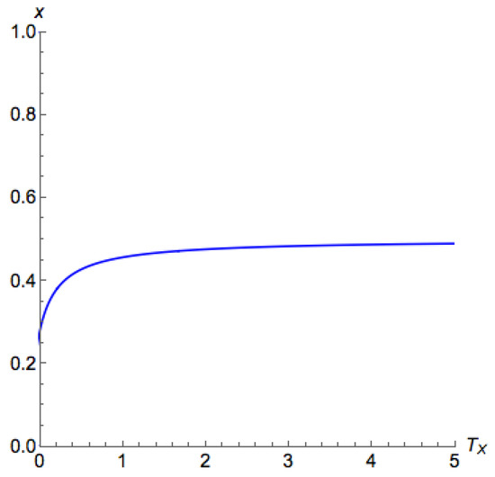
Figure A1.
Bifurcation diagram for a game with no dominating strategy for the first player, , and a low .
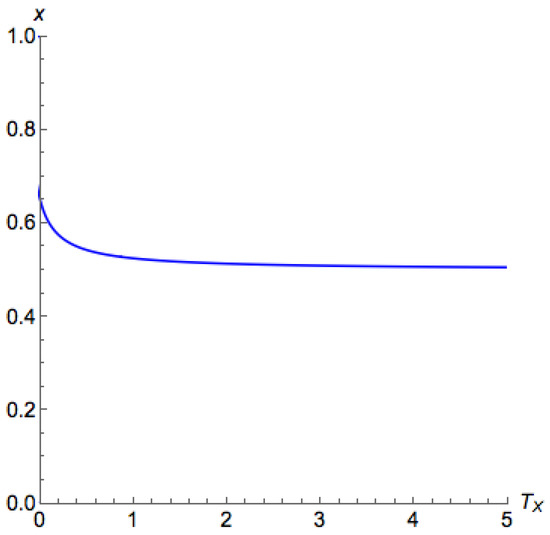
Figure A2.
Bifurcation diagram for a game with no dominating strategy for the first player, , and a high .
Theorem A5.
Given a game in which the diagonal form has , , QRE is unique given and .
Appendix C.2. Dominating Strategy for the First Player
Finally, we consider the case when there is a dominating strategy for the first player, i.e., . According to Figure A3 and Figure A4, the principal branch seems always goes towards . This means that the first player always prefers his/her dominating strategy. We formalize this observation, as well as some important characteristics for this case in the theorem below, where the proof can be found in Appendix D.2 in the appendix.

Figure A3.
Bifurcation diagram for a game with one dominating strategy for the first player and .
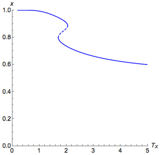
Figure A4.
Bifurcation diagram for a game with one dominating strategy for the first player, , and .
Theorem A6.
Given a game in which the diagonal form has , , , and, given , the following statements are true:
- 1.
- The region contains the principal branch.
- 2.
- There is no QRE correspondence for .
- 3.
- If or , then the principal branch is continuous.
- 4.
- If and , then the principal branch may not be continuous.
As we can see from Theorem A6, for most cases, the principal branch is continuous. One special case is when with . In fact, this can be seen as a duality, i.e., flipping the role of two players, of the case we have discussed in Part 3 of Theorem A4, where, if is within and , there can be three QRE correspondences.
Appendix D. Detailed Bifurcation Analysis for General 2 × 2 Game
In this section, we provide technical details for the results we stated in Section 4.3 and Appendix C. Before we get into details, we state some results that will be useful throughout the analysis in the following lemma. The proof of this lemma is straightforward and we omit it in this paper.
Lemma A2.
The following statements are true.
- 1.
- The derivative of is given aswhere
- 2.
- The derivative of is given as
- 3.
- For , if and only if ; on the other hand, if and only if .
Appendix D.1. Case 1: bX ≥ 0
First, we consider the case . As we are going to show in Proposition A1, the direction of the principal branch relies on , which is the strategy the second player is performing, assuming the first player is indifferent to his/her payoff. The idea is that if is large, then it means that the second player pays more attention to the action that the first player thinks is better. This is more likely to happen when the second player has less rationality, i.e., high temperature . On the other hand, if the second player pays more attention to the other action, the first player is forced to choose that as it gets more expected payoff.
We show that, for , the principal branch lies on ; otherwise, the principal branch lies on . This result follows from the following proposition:
Proposition A1.
For Case 1, if , then ; hence,
On the other hand, if , then ; hence,
Proof.
First, consider the case where , then, for ,
Then, for the case where ,
For the case where , since we assumed ,
As a result, the numerator of Equation (6) at is negative for , which proves the first two limits.
For the remaining two limits, we only need to consider the case ; otherwise, , which is meaningless. For and ,
This makes the numerator of Equation (6) at positive and proves the last two limits.
Appendix D.1.1. Case 1a: bX ≥ 0, aY + bY > 0
In this section, we consider a relaxed version of the class of coordination game as in Section 4.3. We prove theorems presented in Section 4.3, showing that these results can in fact be extended to the case where , instead of requiring and .
First, , is an increasing function of x, meaning
This implies that both players tend to agree to each other. Intuitively, if , then both players agree that the first action is the better one. For this case, we can show that, no matter what is, the principal branch lies on . In fact, this can be extended to the case whenever , which is the first part of Theorem 1.
Proof of Part 1 of Theorem 1.
We can find that, for , for any according to Proposition A1. Since is monotonically increasing with x, for . This means that for any . Additionally, it is easy to see that . As a result, contains the principal branch. ☐
For Case 1a with , on the principal branch, the lower the , the closer x is to 1. We are able to show these monotonicity characteristics in Proposition A2, and they can be used to justify the stability owing to Lemma 1.
Proposition A2.
In Case 1a, if , then for .
Proof.
It suffices to show that for . Note that, according to Proposition A1, if ,
Since is monotonically increasing when , for . As a result, ; hence, we can see that, for ,
Consequently, for , ; hence, according to Lemma A2.
Proof of Part 1 of Theorem 3.
According to Lemma 1, Proposition A2 implies that all is on the principal branch. This directly leads us to Part 1 of Theorem 3. ☐
Next, if we look into the region , we can find that, in this region, QREs appears only when and are low. This observation can be formalized in the proposition below. We can see that this proposition directly proves Parts 2 and 3 of Theorem 2, as well as Part 2 of Theorem 3.
Proposition A3.
Consider Case 1a. Let and . The following statements are true for :
- 1.
- If , then .
- 2.
- If , then if and only if .
- 3.
- for .
- 4.
- If , then .
- 5.
- If , then there is a nonnegative critical temperature such that for . If , then is given as , where is the unique solution to .
Proof.
For the first and second part, consider any and we can see that
Note that for , we have ; hence, .
From the above derivation, for all such that , since . Then
Further, when , . This implies that, for , . Since , and L is continuous, for . This implies the fourth part of the proposition.
Next, if we look at the derivative of ,
We can see that any critical point in must satisfy . When , , and . If , then . Hence, there is exactly one critical point for for , which is a local maximum for . If , then we can see that is always negative, in which case the critical temperature is zero. ☐
The results in Proposition A3 not only apply for the case but also general cases about the characteristics on . According to this proposition, we can conclude the following for the case , as well as the case when :
- The temperature determines whether there is a branch appears in .
- There is some critical temperature . If we raise above , then the system is always on the principal branch.
- The critical temperature is given as the solution to the equality .
When there is a positive critical temperature, though it has no closed form solution, we can perform a binary search to look for that satisfies .
Another result we are able to obtain from Proposition A3 is that the principal branch for Case 1a when lies on .
Proof of Part 2 of Theorem 1.
First, we note that is meaningful only when , for which case we always have . From Proposition A3, we can see that for , we have ; hence, for . From Proposition A1, we already have . Additionally, it is easy to see that . As a result, since is continuously differentiable over , for any , there exists such that . ☐
What remains to be shown is the characteristics on the side when . In Figure 4 and Figure 5, for low , the branch on the side demonstrated a similar behavior as what we have shown in Proposition A3 for the side . However, for a high , while we still can find that contains the principal branch, the principal branch is not continuous. These observations are formalized in the following proposition. From this proposition, the proof of Part 4 of Theorem 2 directly follows.
Proposition A4.
Consider Case 1a with . Let and . The following statements are true for .
- If , then .
- If , then if and only if .
- For , we have .
- If , then there is a positive critical temperature such that for , given as , where is the unique solution of .
Proof.
For the first part and the second part, consider , and we can find that
Note that, for , . Additionally, if , then for all .
For the third part, for all and . Thus,
For the fourth part, we can find that any critical point of in must be either or satisfies the following equation:
Consider . For , is strictly less than . Additionally, . Now, and . Next, we can see that is monotonically decreasing with respect to x for by looking at its derivative:
As a result, there is some such that . This implies that has exactly one critical point for . Additionally, if , ; if , then . Therefore, is a local minimum for L.
From the above arguments, we can conclude that the shape of for is as follows:
- There is a local maximum at , where .
- L is decreasing on the interval , where is the unique solution to Equation (A7).
- L is increasing on the interval . If , then .
Finally, we can claim that there is a unique solution to , and such a point gives a local maximum to . ☐
The above proposition suggests that, for , we are able to use binary search to find the critical temperature. For , unfortunately, with a similar argument of Proposition A4, we can find that there are potentially at most two critical points for on , as shown in Figure 5, which may induce an unstable segment between two stable segments. This also proves Part 3 of Theorem 3.
Now, we have enough materials to prove the remaining statements in Section 4.3.
Proof of Parts 1, 5, and 6 of Theorem 2, Part 4 of Theorem 3.
For , by Proposition A3, we can conclude that, for , we have , for which the QREs are stable by Lemma 1. With similar arguments, we can conclude that the QREs on are unstable. Additionally, given , the stable QRE and the unstable that satisfies appear in pairs. For , with the same technique and by Proposition A4, we can claim that the QREs in are unstable, while the QREs in are stable. This proves the first part of Theorem 2 and Part 4 of Theorem 3.
Parts 5 and 6 of Theorem 2 are corollaries of Part 5 of Proposition A3 and Part 4 of Proposition A4. ☐
Appendix D.1.2. Case 1b: bX > 0, aY + bY < 0
In this case, both players have different preferences. For the game within this class, there is only one Nash equilibrium (either pure or mixed). We presented examples in Figure A1 and Figure A2. We can see that, in these figures, there is only one QRE given and . We show in the following two propositions that this observation is true for all instances.
Proposition A5.
Consider Case 1b. Let . If , then the following statements are true:
- 1.
- for .
- 2.
- for .
- 3.
- for .
- 4.
- contains the principal branch.
Proof.
Note that, if , . Additionally, according to Proposition A2, . Since is continuous and monotonically decreasing with x, for . Therefore, the numerator of Equation (6) is always positive for , which makes negative. This proves the first part of the proposition.
For the second part, observe that, for , if and only if . This is equivalent to .
For the third part, note that, for , . This implies for , from which we can conclude that .
Finally, we note that if , then . If , we have . As a result, we can conclude that contains the principal branch. ☐
With the similar arguments, we are able to show the following proposition for :
Proposition A6.
Consider Case 1b. Let . If , then the following statements are true:
- 1.
- for .
- 2.
- for .
- 3.
- for .
- 4.
- contains the principal branch.
Appendix D.1.3. Case 1c: aY + b + Y = 0
In this case, we have , and is a constant with respect to x. The proof of Theorem A5 for directly follows from the following proposition.
Proposition A7.
Consider Case 1c. The following statements are true:
- 1.
- If , then for , and for .
- 2.
- If , then for , and for .
- 3.
- If , then for .
- 4.
- If , then for .
Proof.
Note that .
First consider the case when . In this case, and . Therefore, , from which we can conclude that for and for , for any positive .
Now consider the case where . If , ; hence, we get for and for , which is the first part of the proposition statement. Similarly, if , , from which the second part of the proposition follows.
For the third part and the fourth part, note that in this case, as as per Equation (A5), and the sign of the derivative of can be seen from Lemma A2. ☐
Appendix D.2. Case 2: bX < 0
In this case, the first action is a dominating strategy for the first player. Note that both and are not positive, which means that the numerator of Equation (6) is always smaller than or equal to zero. This implies that all QRE correspondences appear on . In fact, since for , the numerator of Equation (6) is always negative, we have for . Additionally, we can easily see that
This implies that contains the principal branch. First, we show the result when in the following proposition. Additionally, the bifurcation diagram is presented in Figure A3.
Proposition A8.
For Case 2, if , then for , .
Proof.
In this case, is monotonically decreasing with x. We can see that
since is positive for . Bringing this back to Equation (A4), we have . ☐
For , if , the bifurcation diagram has the similar trend as in Figure A3; while, if , we lose the continuity on the principal branch.
Proposition A9.
For Case 2, if , then for , we have
- 1.
- if , then .
- 2.
- if , then has at most two local extrema.
Proof.
In this case, is monotonically increasing with x. For , we can find that and . Additionally, we can obtain that L is monotonically increasing for by inspecting
Hence, for , . This implies for .
For the second part, we can find that, for , . Let . First note that, if , then, for , we have , and further we can get for . We use the same technique as in the proof of Proposition A4. Let . Note that and . Next, observe that is monotonically decreasing for . Hence, there is an such that . This is a local minimum for L. We can conclude that, for , L has the following shape:
- There is a local maximum at , where .
- L is decreasing on the interval , where is the solution to .
- L is increasing on the interval . Note that .
As a result, if , then is monotonically decreasing; otherwise, has a local minimum and a local maximum on . ☐
References
- Devaney, R.L. A First Course in Chaotic Dynamical Systems; Westview Press: Boulder, CO, USA, 1992. [Google Scholar]
- Roughgarden, T. Intrinsic robustness of the price of anarchy. In Proceedings of the 41st Annual ACM Symposium on Theory of Computing (STOC 2009), Bethesda, MD, USA, 31 May–2 June 2009; pp. 513–522. [Google Scholar]
- Palaiopanos, G.; Panageas, I.; Piliouras, G. Multiplicative weights update with constant step-size in congestion games: Convergence, limit cycles and chaos. In Proceedings of the Advances in Neural Information Processing Systems, Long Beach, CA, USA, 4–9 December 2017; pp. 5874–5884. [Google Scholar]
- Watkins, C.J.C.H. Learning from Delayed Rewards. Ph.D Thesis, University of Cambridge, Cambridge, UK, 1989. [Google Scholar]
- Watkins, C.J.; Dayan, P. Q-learning. Mach. Learn. 1992, 8, 279–292. [Google Scholar] [CrossRef]
- Tan, M. Multi-agent reinforcement learning: Independent vs. cooperative agents. In Proceedings of the tenth international conference on machine learning, Amherst, MA, USA, 27–29 June 1993; pp. 330–337. [Google Scholar]
- McKelvey, R.D.; Palfrey, T.R. Quantal response equilibria for normal form games. Games Econ. Behav. 1995, 10, 6–38. [Google Scholar] [CrossRef]
- Nash, J. Equilibrium points in n-person games. Proc. Natl. Acad. Sci. USA 1950, 36, 48–49. [Google Scholar] [CrossRef] [PubMed]
- Wolpert, D.H.; Harré, M.; Olbrich, E.; Bertschinger, N.; Jost, J. Hysteresis effects of changing the parameters of noncooperative games. Phys. Rev. E 2012, 85, 036102. [Google Scholar] [CrossRef] [PubMed]
- Kianercy, A.; Veltri, R.; Pienta, K.J. Critical transitions in a game theoretic model of tumour metabolism. Interface Focus 2014, 4, 20140014. [Google Scholar] [CrossRef] [PubMed]
- Cominetti, R.; Melo, E.; Sorin, S. A payoff-based learning procedure and its application to traffic games. Games Econ. Behav. 2010, 70, 71–83. [Google Scholar] [CrossRef]
- Coucheney, P.; Gaujal, B.; Mertikopoulos, P. Entropy-Driven Dynamics and Robust Learning Procedures in Games. Available online: https://hal.inria.fr/hal-00790815/document (accessed on 25 April 2018).
- Sato, Y.; Crutchfield, J.P. Coupled replicator equations for the dynamics of learning in multiagent systems. Phys. Rev. E 2003, 67, 015206. [Google Scholar] [CrossRef] [PubMed]
- Tuyls, K.; Verbeeck, K.; Lenaerts, T. A selection-mutation model for q-learning in multi-agent systems. In Proceedings of the 2nd international joint conference on Autonomous agents and multiagent systems, Melbourne, Australia, 14–18 July 2003; pp. 693–700. [Google Scholar]
- Sandholm, W.H. Evolutionary game theory. In Encyclopedia of Complexity and Systems Science; Springer: Berlin, Germany, 2009; pp. 3176–3205. [Google Scholar]
- Kianercy, A.; Galstyan, A. Dynamics of Boltzmann q learning in two-player two-action games. Phys. Rev. E 2012, 85, 041145. [Google Scholar] [CrossRef] [PubMed]
- Hofbauer, J.; Hopkins, E. Learning in perturbed asymmetric games. Games Econ. Behav. 2005, 52, 133–152. [Google Scholar] [CrossRef][Green Version]
- Hofbauer, J.; Sigmund, K. Evolutionary Games and Population Dynamics; Cambridge University Press: Cambridge, UK, 1998. [Google Scholar]
- Perko, L. Differential Equations and Dynamical Systems, 3rd ed.; Springer: Berlin, Germany, 1991. [Google Scholar]
- Tomlinson, I.; Bodmer, W. Modelling the consequences of interactions between tumour cells. Br. J. Cancer 1997, 75, 157–160. [Google Scholar] [CrossRef] [PubMed]
- Kaznatcheev, A.; Scott, J.G.; Basanta, D. Edge effects in game-theoretic dynamics of spatially structured tumours. J. R. Soc. Interface 2015, 12, 20150154. [Google Scholar] [CrossRef] [PubMed]
- Basanta, D.; Scott, J.G.; Fishman, M.N.; Ayala, G.; Hayward, S.W.; Anderson, A.R. Investigating prostate cancer tumour–stroma interactions: Clinical and biological insights from an evolutionary game. Br. J. Cancer 2012, 106, 174–181. [Google Scholar] [CrossRef] [PubMed]
- Kaznatcheev, A.; Velde, R.V.; Scott, J.G.; Basanta, D. Cancer treatment scheduling and dynamic heterogeneity in social dilemmas of tumour acidity and vasculature. arXiv, 2016; arXiv:1608.00985. [Google Scholar]
- Basanta, D.; Simon, M.; Hatzikirou, H.; Deutsch, A. Evolutionary game theory elucidates the role of glycolysis in glioma progression and invasion. Cell Prolif. 2008, 41, 980–987. [Google Scholar] [CrossRef] [PubMed]
- Hanahan, D.; Weinberg, R.A. The hallmarks of cancer. Cell 2000, 100, 57–70. [Google Scholar] [CrossRef]
- Axelrod, R.; Axelrod, D.E.; Pienta, K.J. Evolution of cooperation among tumor cells. Proc. Natl. Acad. Sci. USA 2006, 103, 13474–13479. [Google Scholar] [CrossRef] [PubMed]
- Hanahan, D.; Weinberg, R.A. Hallmarks of cancer: The next generation. Cell 2011, 144, 646–674. [Google Scholar] [CrossRef] [PubMed]
- Ribeiro, M.; Silva, A.S.; Bailey, K.M.; Kumar, N.B.; Sellers, T.A.; Gatenby, R.A.; Ibrahim-Hashim, A.; Gillies, R.J. Buffer Therapy for Cancer. J. nutr. Food Sci. 2012, 2, 6. [Google Scholar] [CrossRef] [PubMed]
- Piliouras, G.; Nieto-Granda, C.; Christensen, H.I.; Shamma, J.S. Persistent Patterns: Multi-agent Learning Beyond Equilibrium and Utility. In Proceedings of the 2014 international conference on Autonomous agents and multi-agent systems (AAMAS), Paris, France, 5–9 May 2014; pp. 181–188. [Google Scholar]
- Papadimitriou, C.; Piliouras, G. From Nash Equilibria to Chain Recurrent Sets: Solution Concepts and Topology. In Proceedings of the 2016 ACM Conference on Innovations in Theoretical Computer Science, Cambridge, MA, USA, 14–16 January 2016; pp. 227–235. [Google Scholar]
- Panageas, I.; Piliouras, G. Average case performance of replicator dynamics in potential games via computing regions of attraction. In Proceedings of the 2016 ACM Conference on Economics and Computation, Maastricht, The Netherlands, 24–28 July 2016; pp. 703–720. [Google Scholar]
- Bloembergen, D.; Tuyls, K.; Hennes, D.; Kaisers, M. Evolutionary dynamics of multi-agent learning: A survey. J. Artif. Intell. Res. 2015, 53, 659–697. [Google Scholar]
- Romero, J. The effect of hysteresis on equilibrium selection in coordination games. J. Econ. Behav. Organ. 2015, 111, 88–105. [Google Scholar] [CrossRef]
- Kleinberg, R.; Ligett, K.; Piliouras, G.; Tardos, É. Beyond the Nash equilibrium barrier. In Proceedings of the Symposium on Innovations in Computer Science (ICS), Beijing, China, 7–9 January 2011. [Google Scholar]
- Piliouras, G.; Shamma, J.S. Optimization Despite Chaos: Convex Relaxations to Complex Limit Sets via Poincaré Recurrence. In Proceedings of the Symposium of Discrete Algorithms (SODA), Portland, OR, USA, 5–7 January 2014. [Google Scholar]
- Kleinberg, R.; Piliouras, G.; Tardos, É. Multiplicative Updates Outperform Generic No-Regret Learning in Congestion Games. In Proceedings of the ACM Symposium on Theory of Computing (STOC), Bethesda, MD, USA, 31 May–2 June 2009. [Google Scholar]
- Mehta, R.; Panageas, I.; Piliouras, G.; Yazdanbod, S. The Computational Complexity of Genetic Diversity. In Proceedings of the 24th Annual European Symposium on Algorithms (ESA 2016), Aarhus, Denmark, 22–24 August 2016; Sankowski, P., Zaroliagis, C., Eds.; Leibniz International Proceedings in Informatics (LIPIcs). Schloss Dagstuhl–Leibniz-Zentrum fuer Informatik: Dagstuhl, Germany, 2016; Volume 57, p. 65. [Google Scholar]
- Livnat, A.; Papadimitriou, C.; Dushoff, J.; Feldman, M.W. A mixability theory for the role of sex in evolution. Proc. Natl. Acad. Sci. USA 2008, 105, 19803–19808. Available online: http://www.pnas.org/content/105/50/19803.full.pdf+html (accessed on 20 April 2018). [CrossRef] [PubMed]
- Chastain, E.; Livnat, A.; Papadimitriou, C.H.; Vazirani, U.V. Multiplicative updates in coordination games and the theory of evolution. In Proceedings of the 4th Innovations in Theoretical Computer Science (ITCS) conference, Berkeley, CA, USA, 10–12 January 2013; pp. 57–58. [Google Scholar]
- Chastain, E.; Livnat, A.; Papadimitriou, C.; Vazirani, U. Algorithms, games, and evolution. Proc. Natl. Acad. Sci. USA 2014, 111, 10620–10623. Available online: http://www.pnas.org/content/early/2014/06/11/1406556111.full.pdf+html (accessed on 20 April 2018). [CrossRef] [PubMed]
- Livnat, A.; Papadimitriou, C.; Rubinstein, A.; Valiant, G.; Wan, A. Satisfiability and evolution. In Proceedings of the 2014 IEEE 55th Annual Symposium on Foundations of Computer Science (FOCS), Philadelphia, PA, USA, 18–21 October 2014; pp. 524–530. [Google Scholar]
- Meir, R.; Parkes, D. A Note on Sex, Evolution, and the Multiplicative Updates Algorithm. In Proceedings of the 12th International Joint Conference on Autonomous Agents and Multiagent Systems (AAMAS 15), Istanbul, Turkey, 4–8 May 2015. [Google Scholar]
- Mehta, R.; Panageas, I.; Piliouras, G. Natural Selection as an Inhibitor of Genetic Diversity: Multiplicative Weights Updates Algorithm and a Conjecture of Haploid Genetics. In Proceedings of the 2015 Conference on Innovations in Theoretical Computer Science, ITCS 2015, Rehovot, Israel, 11–13 January 2015. [Google Scholar]
- Mehta, R.; Panageas, I.; Piliouras, G.; Tetali, P.; Vazirani, V.V. Mutation, Sexual Reproduction and Survival in Dynamic Environments. In Proceedings of the 2017 Conference on Innovations in Theoretical Computer Science (To Appear), ITCS’ 17, Berkeley, CA, USA, 9–11 January 2017. [Google Scholar]
- Livnat, A.; Papadimitriou, C. Sex as an algorithm: The theory of evolution under the lens of computation. Commun. ACM (CACM) 2016, 59, 84–93. [Google Scholar] [CrossRef]
- Sandholm, W.H. Population Games and Evolutionary Dynamics; MIT Press: Cambridge, MA, USA, 2010. [Google Scholar]
- Bendixson, I. Sur les courbes définies par des équations différentielles. Acta Math. 1901, 24, 1–88. [Google Scholar] [CrossRef]
- Teschl, G. Ordinary Differential Equations and Dynamical Systems; American Mathematical Soc.: Providence, RI, USA, 2012; Volume 140. [Google Scholar]
- Müller, J.; Kuttler, C. Methods and Models in Mathematical Biology; Springer: Berlin, Germany, 2015. [Google Scholar]
- Meiss, J. Differential Dynamical Systems; SIAM: Philadelphia, PA, USA, 2007. [Google Scholar]
| 1 | Mixed strategies in the QRE model are sometimes interpreted as frequency distributions of deterministic actions in a large population of users. This population interpretation of mixed strategies is standard and dates back to Nash [8]. Depending on context, we will use either the probabilistic interpretation or the population one. |
| 2 | To find the matrix of the orthogonal projection onto (or any subspace Y of ) it suffices to find a basis (). Let B be the matrix with columns ; then . |
| 3 | A function f between two topological spaces is called a diffeomorphism if it has the following properties: f is a bijection, f is continuously differentiable, and f has a continuously differentiable inverse. Two flows and are diffeomorhpic if there exists a diffeomorphism such that for each and . If two flows are diffeomorphic, then their vector fields are related by the derivative of the conjugacy. That is, we get precisely the same result that we would have obtained if we simply transformed the coordinates in their differential equations [50]. |
© 2018 by the authors. Licensee MDPI, Basel, Switzerland. This article is an open access article distributed under the terms and conditions of the Creative Commons Attribution (CC BY) license (http://creativecommons.org/licenses/by/4.0/).