Evolution of Decisions in Population Games with Sequentially Searching Individuals

Abstract

In many social situations, individuals endeavor to find the single best possible partner, but are constrained to evaluate the candidates in sequence. Examples include the search for mates, economic partnerships, or any other long-term ties where the choice to interact involves two parties. Surprisingly, however, previous theoretical work on mutual choice problems focuses on finding equilibrium solutions, while ignoring the evolutionary dynamics of decisions. Empirically, this may be of high importance, as some equilibrium solutions can never be reached unless the population undergoes radical changes and a sufficient number of individuals change their decisions simultaneously. To address this question, we apply a mutual choice sequential search problem in an evolutionary game-theoretical model that allows one to find solutions that are favored by evolution. As an example, we study the influence of sequential search on the evolutionary dynamics of cooperation. For this, we focus on the classic snowdrift game and the prisoner’s dilemma game.

1. Introduction

The problem of mutual choice was first introduced in the economic literature by [1], who studied how to pair students with colleges so that the preference of both sides would be satisfied. Their framework, further developed in [2,3,4,5,6,7], assumes that there exists a sort of central processor that carries out the pairing. In natural populations, and often in human societies, however, the pairing of individuals happens in a more decentralized and random fashion [8]. For example, the composition of the employee-employer pair who end up concluding a contract depends on who happens to read the job advertisement and in which order the applicants come for the interview. To account for this, theoretical work on sequential and random encounters has been developed and applied to mutual choice problems, such as mate choice [9,10,11,12,13,14] and labor markets [15,16,17,18]. The main focus in sequential search problems, either with mutual or one-sided choice (e.g., female choice only) is to find decision rules that determine the acceptance or rejection of possible partners in such a way that no individual is better off by changing its rule. Thus, if the search season is finite, individuals must find a balance between waiting for a beneficial interaction by rejecting unfavorable ones, while not waiting too long so as not to remain without a partner and no payoff [19,20,21,22,23,24]. However, if the choice is mutual, the model is not a mere optimization problem, and so, there may be multiple solutions [12]. The drawback here is that there is no way of knowing which solution populations will actually reach, if any. That is, we may be able to calculate what individuals should do, but we do not know the solution followed by evolution.

On the other end of the spectrum, we have evolutionary game theory, which has been specifically developed to address evolutionary properties of decisions (e.g., whether to cooperate or defect). However, even though previous work has explored various forms of optional interactions and partner choice, particularly in the theory of the evolution of cooperation [25,26,27,28,29,30,31,32], trade-offs arising from sequential search problems have not been studied. In this paper, we address this issue by embedding a mutual choice sequential search problem to an evolutionary game-theoretical framework, and look for decisions that are favored by evolution. Moreover, we investigate how such social situations affect the evolution of cooperation.

We assume that all individuals are one of two types, cooperators or defectors, where each individual is equipped with a decision rule that dictates throughout the search season whether an encountered individual will be accepted or rejected for an interaction. The search season is assumed to consist of discrete time steps, or rounds, such that at each round, all individuals are being paired. Once an interaction is mutually accepted the interacting individuals drop out of the game pool and will not be available for future rounds. We look for decisions that are favored by evolution and study, on the one hand, how costs are associated with the search process and, on the other hand, how mistakes in evaluating the type of the opponent influence the results. For analytical results, we work out an example where we consider a search season with two rounds and give conditions for which we find unique, multiple or no stable dynamic equilibria, in which case, an evolutionary cycling occurs. Furthermore, similarly to the previous work on optional interactions and partner choice, we find that the option to refuse an interaction always favors cooperators. Interestingly, if the search for new opponents is considered to be costly, high levels of cooperation may evolve even in the prisoner’s dilemma, where for obligatory interactions, defection yields the highest payoff. This is because discriminated defectors have to on average search longer for an accepted interaction than cooperators and, thus, pay higher costs associated with search. However, mistakes in evaluating the type of opponent favor defection, because even if defectors are being discriminated against, they may be accepted by mistake.

2. The General Model

Consider an infinitely large and well-mixed population where each individual is either a cooperator (C) or a defector (D). In every generation, each individual is about to enter a maximum of $M\in N_{+}$ rounds, such that at each round, individuals are pitted against each other and given a choice to interact. Encountered players are said to interact if they both decide to accept an offer from each other, in which case their search for new opponents is terminated, and they receive a strictly positive payoff according to a payoff matrix (see the section below). If, however, at least one of the two individuals decides not to interact, i.e., she declines the offer from the opponent, both will move to the next round and will be randomly assigned a new opponent. If an individual declines all of the offers or if she will be declined, she will receive a zero payoff. In every generation, all individuals thus participate in at most one interaction (i.e., play at most one one-shot game). The frequency distribution of the next generation is updated based on the payoffs received in the parent generation.

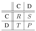
2.1. Payoffs

Individuals that engage in an interaction, i.e., accept an offer from each other) receive a payoff according to their types: if at least one of the two interacting individuals is a cooperator, a benefit $2b$ is produced and shared equally (b for each player). A cooperator pays a cost c for his cooperation, which is divided if both individuals are cooperators, in which case each pays $\frac{c}{2}$. Defectors do not pay costs, but if both individuals are defectors, then no benefit is produced. In addition, we assume that playing a game, even if against an unfavorable opponent, is more beneficial than remaining without an opponent. We implement this by considering an additional payoff u (see, e.g., [31]) so that all individuals that play a game receive a strictly positive payoff. For example, we may think of interactions that themselves have a value, such as offspring production. Clearly, individuals that produce offspring, even with a defector, are better off than when not reproducing at all.

By setting $c=kb$, where k describes how many times the cost of cooperation is greater than the benefit, we recover the snowdrift game (SD) for $0<k<1$ (i.e., $0<c<b$) and the prisoner’s dilemma (PD) for $1<k<2$ (i.e., $b<c<2b$). The payoff matrix for an accepted game is thus:

where $T=b,R=b(1-\frac{1}{2}k),S=b(1-k)$, $P=0$, with the additional payoff u, so that all the payoffs are strictly positive. Finally, entering each new round may be costly (e.g., the cost of search), and therefore, a will be subtracted per each entered (not necessarily accepted) round. Throughout the paper, we will use k as our main model parameter.

2.2. Decisions, Types and Strategies

For both games, SD and PD, the ideal opponent is a cooperator (i.e., $R>S$ and $T>P$), and so the best decision, for both types C and D, is to always accept an opponent of type C. The question is therefore in which rounds an encountered type D should be accepted for the payoff to be maximized. This is not trivial for two reasons. First, there is a trade-off between interacting with an encountered type D in the current round and the costs associated with waiting to encounter type C in future rounds. Second, since interacting individuals drop out of the game pool, the frequency distribution and hence the expected payoff may change throughout the search season. Therefore, an individual may want to accept (decline) type D in one round, but decline (accept) him in the next.

A decision may be represented as a vector, where each entry is either zero or one, depending on whether in that round an opponent of type D is rejected or accepted, respectively. If M is the maximum number of rounds, then the maximum number of decisions in the population is $N_s=2^M$. We may therefore write the complete set of decisions as:

$$Q=\{q_1,\cdots ,q_{N_s}\},$$

(1)

where $q_j=(q_{j_1},\cdots ,q_{j_M})\in Q$, $1\le j\le N_s$, is a decision vector and where each element $q_{j_i}$ is either a zero or one (i.e., say no or yes, respectively, to an encountered D) at round $1\le i<M$. Each individual possesses a decision vector, and we will denote with $C_i=C_{q_i}$ and $D_j=D_{q_j}$ types C and D, respectively, who use decisions $q_i,q_j\in Q$. We call $C_i,D_j$ strategies that individuals are identified with, and the set of all strategies we denote with S.

2.3. Expected Payoffs and Game Probabilities

Consider maximum M rounds per generation. The expected payoff per generation for strategies $C_j,D_j\in S$ may be written as:

$$\begin{array}{cc}& E_{C_j}=R\sum _{q_i\in Q}{\pi }_{C_j{C}_i}+S\sum _{q_i\in Q}{\pi }_{C_j{D}_i}-a{n}_{C_j},1\le j\le N_s\hfill \end{array}$$

(2a)

$$\begin{array}{cc}& E_{D_j}=T\sum _{q_i\in Q}{\pi }_{D_j{C}_i}+P\sum _{q_i\in Q}{\pi }_{D_j{D}_i}-a{n}_{D_j},1\le j\le N_s,\hfill \end{array}$$

(2b)

where $n_{C_j},n_{D_j}$ are the expected number of rounds that strategies $C_j,D_j$, respectively, have entered and ${\pi }_{C_j{C}_i}$ is the probability that strategy $C_j$ will play against $C_i$. The expected number of rounds may be expressed as:

$$n_A=1·(1-r_{A,1})+2·r_{A,1}(1-r_{A,2})+\cdots =\sum _{i=1}^M\left(i(1-r_{A_i})\prod _{j=1}^{i-1}{r}_{A,j}\right),A\in S,$$

(3)

where $r_{A,i}$ is the probability that in round i, strategy $A\in S$ does not play a game, that is strategy A encounters an opponent who is either not going to be accepted by A and/or who would not accept strategy A. We may write this as:

$$r_{A,i}=\sum _{B\in S}{p}_{B,i}{v}_{AB,i}$$

(4)

where $p_{B,i}$ is the frequency of $B\in S$ in round i and $v_{AB,i}$ is the probability that in round i, upon an encounter between A and B, either strategy A does not accept strategy B and/or B does not accept strategy A (notice that $v_{AB,i}=v_{BA,i}$). This depends on the decision vector, but also on how accurately an individual evaluates the type of opponent. This is model dependent and may, for example, be a function of the reputation of the individuals type or the quality of the signal. In the next section, we analyze a model where in each round, there is a fixed probability ε that a mistake is made in correctly evaluating the type of the opponent (C vs. D). If there is a strictly positive probability $\epsilon >0$ that a mistake is made, we say that the signal of the opponent is imperfect. We assume that the opponent’s decision $q_i\in Q$ is unknown to the individual.

As indicated in Equation (4), frequencies of C and D change from round to round. This is because in each round, some players may accept each other for an interaction and, thus, drop out of the game pool. Since $r_{A,i}$ in Equation (4) can also be interpreted as the fraction of A in round i who enter round $i+1$, we can write the frequency of $A\in S$ at round $i+1$, where $1\le i<M$, as:

$$p_{A,i+1}=p_{A,i}\frac{r_{A,i}}{\overline{p}}$$

(5)

where $\overline{p}={\sum }_{B\in S}{p}_{B,i}{r}_{B,i}$ is the mean absolute frequency. We may now write out the probability that a game is played between strategies $A\in S$ and $B\in S$:

$$\begin{array}{cc}\hfill {\pi }_{AB}& =p_{B,1}(1-v_{AB,1})+r_{A,1}{p}_{B,2}(1-v_{AB,2})+r_{A,1}{r}_{A,2}{p}_{B,3}(1-v_{AB,3})+\cdots \hfill \\ & =\sum _{i=1}^M\left(p_{B,i}(1-v_{AB,i})\prod _{j=1}^{i-1}{r}_{A,j}\right).\hfill \end{array}$$

(6)

2.4. Replicator Equation

We study the evolution of strategies $A\in S$ by applying replicator equations:

$${\dot{p}}_A=p_A\left(E_A-\overline{E}\right),A\in S,$$

(7)

where the dot represents a time derivative, $\overline{E}={\sum }_{B\in S}{p}_B{E}_B$ is the mean expected payoff and ${\sum }_A{p}_A=1$. Notice, that the dynamical system Equation (7) is fully characterized by the functions $v_{AB,i}$. After $v_{AB,i}$ has been found, we can simply substitute it into Equations (2)–Equation (6), and the system Equation (7) is obtained. Furthermore, note that the frequencies at the start of each generation are the frequencies in the first round of the game, i.e., $p_A=p_{A,1}$.

3. The Results

In this section, we look for (pure) strategies $C_i,D_j$, as well as their frequencies $p_{C_i},p_{D_j}$ that are favored by evolution. We analyze the existence of strategies that are uninvadable (evolutionarily-stable strategies or ESS) or that can only be invaded by neutral drift. Since, in the latter case, no other strategy has a selective advantage, i.e., strictly positive growth rate, we call it a best selective strategy (BSS). Jointly with ESS, we call them best strategies. We define a best strategy solution as the frequency distribution over a set of strategies, such that no deviation from this state increases individuals’ payoff. In other words, when the population is at the best strategy solution, no individual is (strictly) better off by changing its strategy. Note that this concept satisfies the conditions of a Nash equilibrium. Moreover, we are interested whether choosy decisions (i.e., decisions where individuals decline interactions) evolve, which best strategy solution, if any, is reached and whether evolution increases the level of cooperation.

To facilitate the analytical treatment, we focus on generations with two rounds ($M=2$). In the final Section 4, we discuss what happens when this assumption is relaxed. Because every mutually-accepted interaction yields a strictly positive payoff (see the payoff matrix in Section 2.1) and declined interaction yields a zero payoff, then at least in the final round, all individuals should accept their opponent. This reduces the number of decisions to only two decisions: either accept or decline a D at Round 1 and accept everyone at Round 2, i.e., $q_1=(1,1)$ and $q_2=(0,1)$. There are thus only four strategies $C_{(1,1)},D_{(1,1)},C_{(0,1)}$ and $D_{(0,1)}$, and we write for short $C_1,D_1,C_0$ and $D_0$, respectively, so that $S=\{C_1,D_1,C_0,D_0\}.$ The dynamical model we will study is:

$$\left\{\begin{array}{cc}& {\dot{p}}_{C_1}=p_{C_1}\left(E_{C_1}-\overline{E}\right)\hfill \\ & {\dot{p}}_{D_1}=p_{D_1}\left(E_{D_1}-\overline{E}\right)\hfill \\ & {\dot{p}}_{C_0}=p_{C_0}\left(E_{C_0}-\overline{E}\right)\hfill \\ & {\dot{p}}_{D_0}=p_{D_0}\left(E_{D_0}-\overline{E}\right)\hfill \end{array}\right.$$

(8)

with ${\sum }_A{p}_A=1$ and where the expected payoffs $E_A$ are obtained from Equation (2) by first calculating $v_{AB,i}$ and then substituting this into Equations (3)–(6). Since, in the last round, everyone is accepted, we have $v_{AB,2}=0$, and for $v_{AB,1}$, we find:

$$\begin{array}{cc}& v_{C_1{C}_1}=0\hfill \\ & v_{C_1{C}_0}=\epsilon \hfill \\ & v_{C_1{D}_1}=0\hfill \\ & v_{C_1{D}_0}=\epsilon \hfill \end{array}\begin{array}{cc}& v_{D_1{C}_1}=0\hfill \\ & v_{D_1{C}_0}=1-\epsilon \hfill \\ & v_{D_1{D}_0}=1-\epsilon \hfill \\ & v_{D_1{D}_1}=0\hfill \end{array}\begin{array}{cc}& v_{C_0{C}_1}=\epsilon \hfill \\ & v_{C_0{C}_0}=1-{(1-\epsilon )}^2\hfill \\ & v_{C_0{D}_0}=1-\epsilon (1-\epsilon )\hfill \\ & v_{C_0{D}_1}=1-\epsilon \hfill \end{array}\begin{array}{cc}& v_{D_0{C}_1}=\epsilon \hfill \\ & v_{D_0{C}_0}=1-\epsilon (1-\epsilon )\hfill \\ & v_{D_0{D}_0}=1-{\epsilon }^2\hfill \\ & v_{D_0{D}_1}=1-\epsilon \hfill \end{array}$$

(9)

where $v_{AB}=v_{AB,1}$.

The best strategies are found by calculating the (dynamic) equilibria of system Equation (8) and analyzing their stability. Asymptotically-stable equilibria are the uninvadable strategies (ESS), and stable, but not asymptotically-stable equilibria are the best selective strategies (BSS). In our model, all BSS are stable, but not asymptotically stable, because they form a (continuous) line of equilibria, so that the dynamics is neutral in one direction of the phase plane, but asymptotically stable in all other directions. We will denote equilibrium frequencies with ${\widehat{p}}_{(·)}$, such that, for example, ${\widehat{p}}_{C_1{D}_0}=(0,p_{C_1},p_{D_0},0)$ denotes an equilibrium where only strategies $C_1$ and $D_0$ have strictly positive frequencies. If there is more than one equilibrium, we enumerate them.

To study whether an evolutionary trajectory converges to a particular best strategy solution, we assume that a new strategy appearing in the population is a much rarer event than other demographic processes, such as strategy inheritance. We thus assume that the population settles at an attractor before a new strategy is introduced into the population. An evolutionary trajectory is thus a sequence of successful invasion events, which we simply call an invasion-substitution sequence. We assume that each invasion-substitution sequence starts from a population where everyone uses non-choosy decisions $q_1=(1,1)$. Since all individuals accept the first encountered interaction, we obtain as the initial state the solutions of the one-shot snowdrift game and the prisoner’s dilemma: for the snowdrift game $0<k<1$, the initial frequency distribution is:

$${\widehat{p}}_{C_1{D}_1}=\left(2\frac{1-k}{2-k},\frac{k}{2-k}\right)$$

(10a)

and for the prisoner’s dilemma $1<k<2$, it is:

$${\widehat{p}}_{D_1}=1.$$

(10b)

In Section 3.1, we analyze a basic model, which assumes no search costs and where the type of opponent is evaluated correctly ($a=0,\epsilon =0$). In Section 3.2, we relax the assumptions by considering the effect of imperfect signals ($\epsilon >0$, with $a=0$), and in Section 3.3, we consider the effect of search costs ($a>0$, with $\epsilon =0$). Lastly, in Section 3.4, we discuss the full model ($\epsilon >0,a>0$). For all models, we first find analytical conditions for choosy strategies $C_0$ and $D_0$ to invade a population that uses only non-choosy decisions (see Equation (10)). If choosy strategies are not able to invade, the initial state given in Equation (10) is the best strategy solution. Next, we find all of the (remaining) best strategy solutions, and investigate to which best strategy solution invasion-substitution sequence converges. The results are summarized in Figure 1, Figure 2, Figure 3 and Figure 4, where each model has its own figure and where each panel gives a simplex spanned by strategies in S with arrows that indicate the direction of the evolutionary dynamics. In addition, we draw grey dashed arrows for each qualitatively different invasion-substitution sequence that our model contains. See the captions, Section 3.1, Section 3.2, Section 3.3 and Section 3.4 and the Appendix for further explanations and discussions.

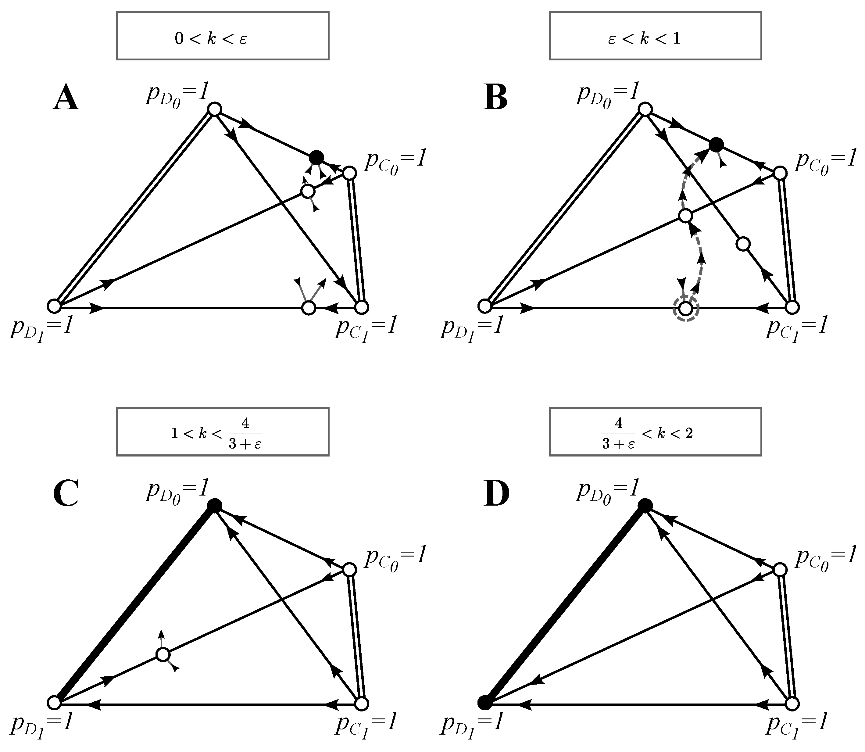
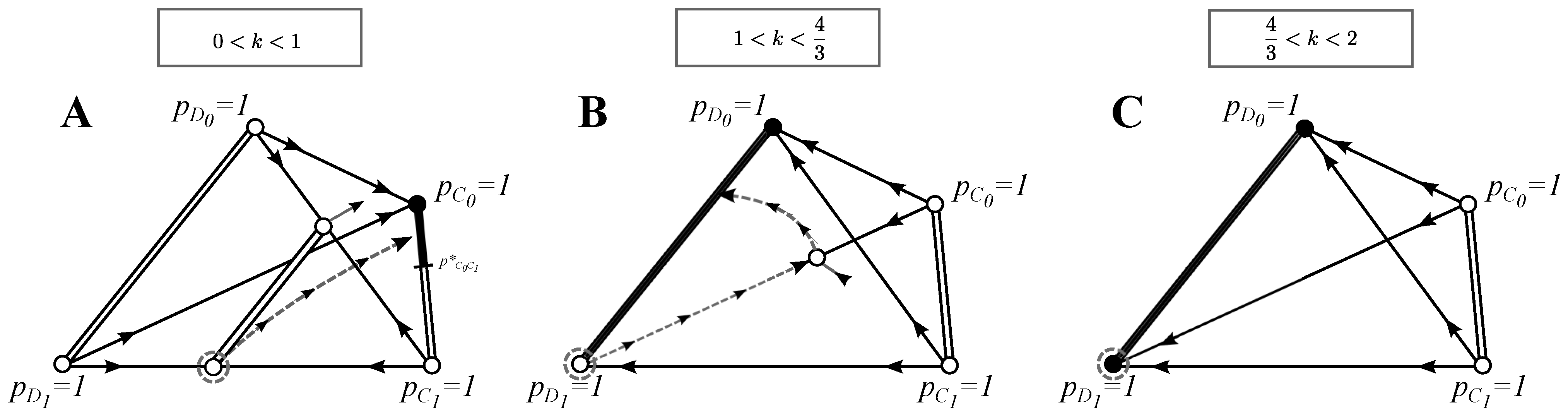
3.1. (A) The Basic Model

In the basic model, we suppose that entering a new round is not costly, $a=0$, and that the type of the opponent (C vs. D) is evaluated correctly, $\epsilon =0$. This model can be fully analyzed analytically. Figure 1 summarizes the results (see Appendix for the full analysis).

Our general finding is that if the benefit from mutual cooperation is high enough (parameter k is not too large), optional interactions favor choosy decisions. This is because by rejecting encountered defectors in the first round, choosy individuals have a chance to interact with a cooperator in the second round. For the snowdrift game, the payoff matrix favors choosy cooperators over choosy (and non-choosy) defectors, and so, cooperation is the winning strategy. In the prisoner’s dilemma, choosy defectors do better than choosy cooperators, and so, defection takes over, even if initially choosy cooperators have an advantage over non-choosy defectors.

Figure 1. Phase plane analysis for the basic model: Each panel presents a simplex where each point is a frequency distribution at some point in time with ${\sum }_A{p}_A=1$. With double-lines, we indicate the set of frequencies where each point is an equilibrium; with black color, we show which equilibrium is stable (not necessarily asymptotically stable) and with white color, which equilibria are unstable. Arrows indicate the direction of the dynamics along each eigenvector. Grey dashed arrows give an example of an invasion-substitution sequence. See Section 3.1 for the discussion of the evolutionary properties of this model and the Appendix for the full analytical treatment.

Figure 1. Phase plane analysis for the basic model: Each panel presents a simplex where each point is a frequency distribution at some point in time with ${\sum }_A{p}_A=1$. With double-lines, we indicate the set of frequencies where each point is an equilibrium; with black color, we show which equilibrium is stable (not necessarily asymptotically stable) and with white color, which equilibria are unstable. Arrows indicate the direction of the dynamics along each eigenvector. Grey dashed arrows give an example of an invasion-substitution sequence. See Section 3.1 for the discussion of the evolutionary properties of this model and the Appendix for the full analytical treatment.

3.1.1. Invasion of Choosy Decisions

Choosy decisions $q_2=(0,1)$ can evolve if rare choosy strategies $C_0$ and/or $D_0$ can invade a non-choosy population Equation (10). We find that for all $0<k<2$, choosy defectors $D_0$ have a zero growth rate and can thus increase in frequency only via neutral drift (see the Appendix and Figure 1). This is simply because the only pairs who go to the second round are defectors $D_0$ and $D_1$, and thus, rejecting a defector in the first round yields no payoff advantage. However, when choosy cooperators $C_0$ are introduced to the population, then in the second round, half of the individuals are choosy cooperators (the other half are defectors), and so, rejecting a defector in the first round gives cooperators an equal chance to eventually interact with a cooperator. We get that $C_0$ can invade the initial population whenever $0<k<\frac{4}{3}$. For $\frac{4}{3}<k<2$, the initial state given in Equation (10) is the best strategy solution. Within this parameter range, the benefit from mutual cooperation is too low to outweigh the fact that with probability one half, a $C_0$ ends up interacting with a D in the second round.

3.1.2. Best Strategies

In this section, we look for best strategy solutions. Each enumeration corresponds to the panels of Figure 1:

(A) $0<k<1$: The best selective strategy is a strategy pair ($C_0,C_1$) that lies on the line of equilibria ${\widehat{p}}_{C_1{C}_0}$ with $k<p_{C_0}\le 1$. This line of equilibria exists because $C_0$ has the same payoff against $C_1$ and vice versa. Interestingly, defectors can invade the strategy pair ($C_0,C_1$) if population drifts past the point $p_{C_0{C}_1}^{*}=k$ (see Figure 1A). Eventually, however, the dynamics will lead defectors to extinction, and a mix of cooperative strategies $(C_0,C_1)$ is again established. This evolutionary cycle, which relies on the absence of selection on the effect of neutral drift, can be written symbolically as $(C_0,C_1)\stackrel{\text{drift}}{\to }(C_0,C_1)\stackrel{\text{invasion}\text{by}{D}_0/D_1}{\to }(C_0,C_1)$. We thus have that a strategy pair $(C_0,C_1)$ can drift from one fully-cooperative equilibrium to another, but after passing a certain threshold value, it can be temporarily invaded by defectors.

(B) $1<k<\frac{4}{3}$: A strategy pair of defectors ($D_0,D_1$) that lies on the line of equilibria ${\widehat{p}}_{D_1{D}_0}$, with $0<p_{D_0}\le 1$, is the best selective strategy. This solution can only be escaped if strategy $D_0$ drifts to complete extinction ($p_{D_0}=0$), after which strategy $C_0$ can invade, and the coexistence of $(D_1,C_0)$ is established at ${\widehat{p}}_{D_1{C}_0}=(p_{D_1},p_{C_0})=(\frac{2(k-1)}{2-k},\frac{4-3k}{2-k})$. However, this state can be invaded by $D_0$, and the strategy pair ($D_0,D_1$) is established again as a BSS, i.e., we have $(D_0,D_1)\stackrel{\text{drift}}{\to }{D}_1\stackrel{\text{invasion}\text{by}{C}_0}{\to }(C_0,D_1)\stackrel{\text{invasion}\text{by}{D}_0}{\to }(D_0,D_1)$.

(C) $\frac{4}{3}<k<2$: Any strategy pair ($D_0,D_1$) that lies on the line of equilibria ${\widehat{p}}_{D_1{D}_0}$ for all $0\le p_{D_0}\le 1$ is a BSS.

3.1.3. Evolution of Cooperation and Choosy Decisions

In this section, we describe all of the invasion-substitution sequences (see the Appendix for the full analysis). As in the previous section, each enumeration corresponds to the panels of Figure 1:

(A) $0<k<1$: The initial population $(C_1,D_1)$, indicated by a grey dashed circle, can be (selectively) invaded by a choosy cooperator $C_0$, but not by a choosy defector $D_0$ (see Section 3.1.1 and Figure 1A). If $C_0$ succeeds at invading, a strategy pair ($C_0$, $C_1$) at ${\widehat{p}}_{C_1{C}_0}$, with $k<p_{C_0}\le 1$, is established as a BSS. The invasion-substitution sequence is thus $(C_1,D_1)\stackrel{\text{invasion}\text{by}{C}_0}{\to }(C_0,C_1)$ (see the dashed grey trajectory drawn in Figure 1A). Recall that this solution can be escaped by neutral drift (see Section 3.1.2).

(B) $1<k<\frac{4}{3}$: The initial population consist of defectors $D_1$ only. If choosy strategies are introduced, $C_0$ may invade and can be established at an equilibrium together with $D_1$, at least, until $D_0$ is introduced, and a strategy pair of defectors $(D_0,D_1)$ at ${\widehat{p}}_{D_1{D}_0}$ with $0<p_{D_0}\le 1$, will be established as a BSS. Interestingly, pure defection takes over the coexistence of ($C_0$, $D_1$) at ${\widehat{p}}_{D_1{C}_0}$ only if defectors start to be choosy against themselves. We have $D_1\stackrel{\text{invasion}\text{by}{C}_0}{\to }(D_1,C_0)\stackrel{\text{invasion}\text{by}{D}_0}{\to }(D_1,D_0)$. This solution may be escaped by drift (see Section 3.1.2).

(C) $\frac{4}{3}<k<2$: No strategy can selectively invade the initial state ${\widehat{p}}_{D_1}=1$. Due to drift, any best strategy solution on the line of equilibria ${\widehat{p}}_{D_1,D_0}$ with $0\le p_{D_1}\le 1$ may be reached.

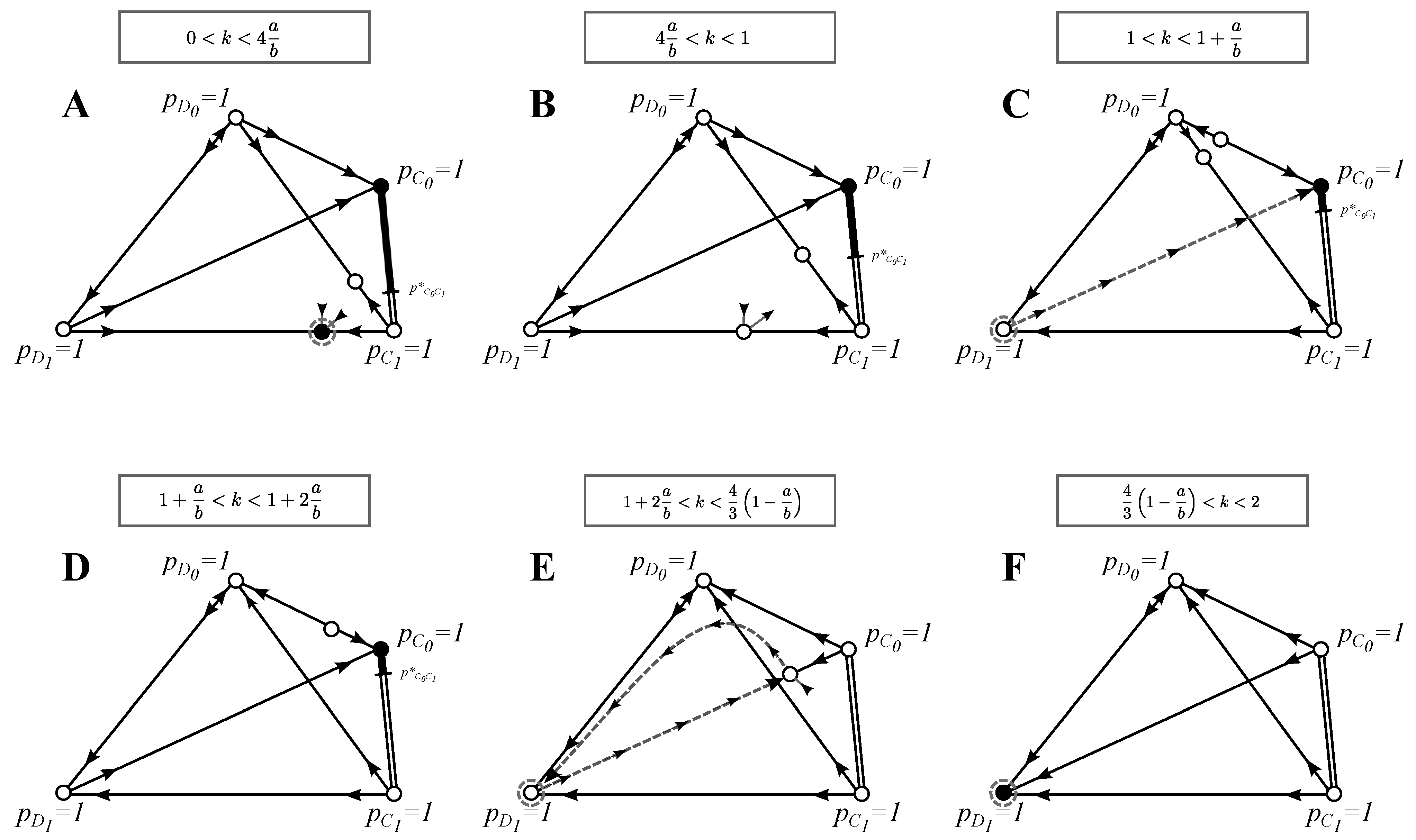
3.2. (B) Imperfect Signals

In this model, we suppose that individuals make a mistake with probability $\epsilon >0$ in evaluating whether the encountered opponent is a cooperator or a defector. We suppose there are no search costs, $a=0$.

The basic model unfolds in three ways when $\epsilon >0$. Firstly, for $0<k<1$, the equilibrium ${\widehat{p}}_{C_0}=1$ becomes unstable. This is because, when most of the individuals are of type $C_0$, i.e., $p_{C_0}$ is close to one, and mistakes are being made, then most of the declined individuals are $C_0$’s, but only mistaken as D’s. Therefore, most of the individuals in the first and second round are $C_0$, and so, defectors, being rare, will end up playing against the common C. Since the payoff for D against C is always greater than C against C, i.e., $R<T$ for all $0<k<2$, defectors can always invade $C_0$ when rare. The reason why this is not true in the basic model for $0<k<1$, is that since no mistakes are made and D’s are rare, only the defector-cooperator pairs go to the second round. Since D’s play in the second round against D and C with equal probability, then for $0<k<1$ we have $\frac{1}{2}(T+P)<R$, and so, defectors cannot invade $C_0$.

The second unfolding happens at $p_{C_1}=1$. In the model with imperfect signals, the equilibrium ${\widehat{p}}_{C_1}=1$ is stable in the direction of $p_{D_0}=1$, for $0<k<\epsilon$, whereas in the basic model, this is always unstable. Because near $p_{C_1}=1$, the choosy defectors $D_0$ encounter mainly $C_1$’s, then fraction $1-\epsilon$ is being accepted, and the game is played. However, fraction ε is declined, and so, in the second round with probability half, the game will be played against another defector. In the basic model, all $D_0$’s play against $C_1$. Thus, in the imperfect signal model, for $0<k<\epsilon$, the cost of playing against another D is greater than the benefit of playing against a C, and so, a rare $D_0$ is not able to invade $C_1$.

Finally, numerical analysis shows that an unstable trimorphic equilibrium ${\widehat{p}}_{C_1{C}_0{D}_0}$ exists for $0<k<1$ (see the Appendix). As it is not the best strategy solution and it does not affect the invasion-substitution dynamics, it is not drawn in Figure 2.

Figure 2. Phase-plane analysis for the model with imperfect signals: see Figure 1 for explanations. In this slightly more complicated model, arrows are not drawn for the dimorphic equilibria (equilibria on the edges) that are not best strategy solutions or that do not affect the invasion substitution sequence. Trimorphic equilibria that are not the best strategy solutions or that do not affect the invasion-substitution sequence are not drawn at all. We found no four-morphic equilibria. Grey dashed arrows give an example of an invasion-substitution sequence. We only draw the sequences that are qualitatively different from the ones presented in Figure 1. See Section 3.2 for the discussion of the evolutionary properties of this model and the Appendix for further analysis.

Figure 2. Phase-plane analysis for the model with imperfect signals: see Figure 1 for explanations. In this slightly more complicated model, arrows are not drawn for the dimorphic equilibria (equilibria on the edges) that are not best strategy solutions or that do not affect the invasion substitution sequence. Trimorphic equilibria that are not the best strategy solutions or that do not affect the invasion-substitution sequence are not drawn at all. We found no four-morphic equilibria. Grey dashed arrows give an example of an invasion-substitution sequence. We only draw the sequences that are qualitatively different from the ones presented in Figure 1. See Section 3.2 for the discussion of the evolutionary properties of this model and the Appendix for further analysis.

3.2.1. Invasion of Choosy Decisions

We find that for $0<k<1$, the initial non-choosy population given in Equation (10) can never be invaded by $D_0$ because its growth rate is negative. For $1<k<2$, the strategy $D_0$ has a zero growth rate and can thus increase in frequency only by neutral drift (Appendix). Strategy $C_0$ can invade ${\widehat{p}}_{C_1{D}_1}$ for all $0<k<1$, and it can invade ${\widehat{p}}_{D_1}$ whenever $1<k<\frac{4}{3+\epsilon }$.

3.2.2. Best Strategies

All of the best strategy solutions (besides the solution ${\widehat{p}}_{D_1}$; see above) are found numerically (see the Appendix for the numerical analysis). Below, the enumeration corresponds to the panels of Figure 2.

(A)–(B) $0<k<1$: Strategy pair ($C_0,D_0$) at the equilibrium ${\widehat{p}}_{C_0{D}_0}$ is an ESS. No other best strategy solutions are found.

(C) $1<k<\frac{4}{3+\epsilon }$: A strategy pair ($D_0,D_1$) on the line of equilibria ${\widehat{p}}_{D_0{D}_1}$, for $0<p_{D_0}\le 1$, is a BSS and the only best strategy solution. A population may move between different values of ${\widehat{p}}_{D_0,D_1}$ due to drift. If $D_0$ becomes extinct, a $C_0$ may invade, and the coexistence of $D_1$ and $C_0$ at ${\widehat{p}}_{D_1{C}_0}$ is established. However, $D_0$ can invade this state, and the best selective strategy solution ($D_0,D_1$) is again established. Neutral drift may thus cause the following cycle: $(D_0,D_1)\stackrel{\text{drift}}{\to }{D}_1\stackrel{\text{invasion}\text{by}{C}_0}{\to }(C_0,D_1)\stackrel{\text{invasion}\text{by}{D}_0}{\to }(D_0,D_1)$.

(D) $\frac{4}{3+\epsilon }<k<2$: A strategy pair ($D_0,D_1$) at any point on the line of equilibria ${\widehat{p}}_{D_0{D}_1}$, $0\le p_{D_0}\le 1$ is a BSS and the only best strategy solution.

3.2.3. Evolution of Cooperation and Choosy Decisions

All of the invasion-substitution sequences were found numerically (see the Appendix). The enumeration corresponds to the panels of Figure 2:

(A)–(B) $0<k<1$: Of the choosy strategies, only $C_0$ is able to invade the initial resident population ${\widehat{p}}_{C_1{D}_1}$, after which a strategy pair $(D_1,C_0)$ is established at ${\widehat{p}}_{D_1{C}_0}$. This state can be invaded by $D_0$, and a stable coexistence of choosy strategies ($C_0,D_0$) is established at ${\widehat{p}}_{C_0,D_0}$. As this is an ESS, it is an evolutionary end point. We have: $(C_1,D_1)\stackrel{\text{invasion}\text{by}{C}_0}{\to }(D_1,C_0)\stackrel{\text{invasion}\text{by}{D}_0}{\to }(C_0,D_0)$.

(C) $1<k<\frac{4}{3+\epsilon }$: Only $C_0$ can selectively invade the initial population ${\widehat{p}}_{D_1}=1$, after which $D_0$ can invade, and a BSS solution ${\widehat{p}}_{D_0,D_1}$, with $0<p_{D_0}\le 1$, is reached. We have $D_1\stackrel{\text{invasion}\text{by}{C}_0}{\to }(D_1,C_0)\stackrel{\text{invasion}\text{by}{D}_0}{\to }(D_1,D_0)$ (the invasion-substitution sequence is qualitatively similar to the one in Figure 1B). This state can only be escaped by neutral drift (see Section 3.2.2).

(D) $\frac{4}{3+\epsilon }<k<2$: No strategy can selectively invade the initial state ${\widehat{p}}_{D_1}=1$. Due to drift, any BSS at equilibrium ${\widehat{p}}_{D_1,D_0}$, with $0\le p_{D_1}\le 1$, may be reached (this case is similar to Figure 1C).

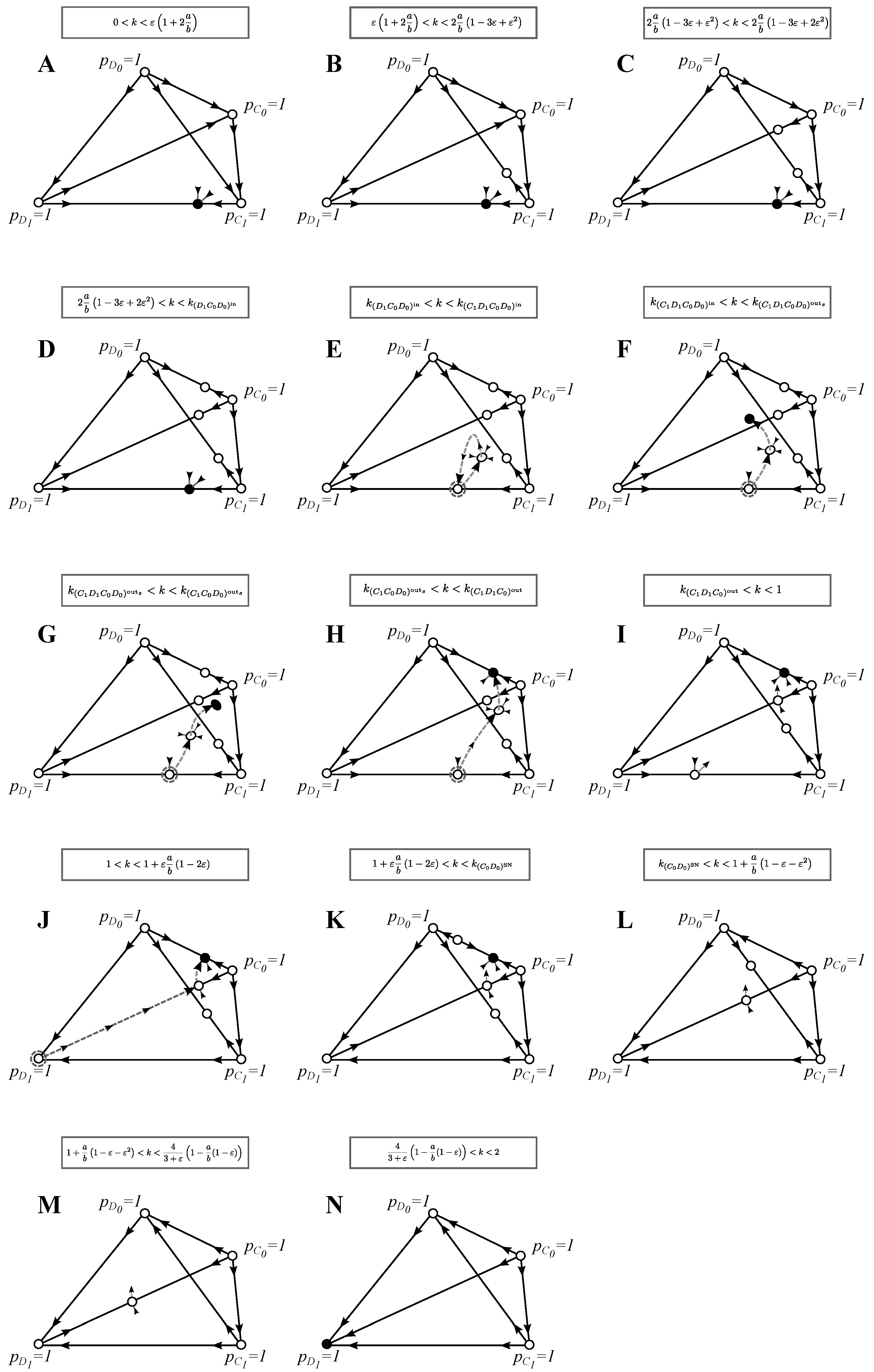
3.3. (C) Search Costs

In this section, we suppose that searching for a new opponent is costly $a>0$, but that no mistakes are made $\epsilon =0$. We analyze in detail a case $0<a<\frac{1}{10}b$ where costs are relatively small compared to the benefit from cooperation. The effect of higher costs is briefly discussed in the paragraph below. When analytical treatment was not possible, we resorted to numerical investigations (see the Appendix).

Search costs bring out a richer bifurcation structure than the basic model (see Figure 3). First of all, the line of equilibria $(p_{D_0},p_{D_1})$ unfolds to a one-directional flow towards $p_{D_1}=1$. This is simply because rounds are costly, and so, accepting a D in the first round is better than accepting D in the second round. This does not happen to the other line of equilibria with only cooperators, because a population of cooperators plays only one round (since $\epsilon =0$, no cooperators are mistaken for defectors). Secondly, the non-choosy population ${\widehat{p}}_{C_1,D_1}$ for $k<4\frac{a}{b}$ cannot be invaded by $C_0$, because the costs of going to the second round are too high compared to the benefit gain from cooperation. Furthermore, numerical analysis shows that there are several trimorphic equilibria, but since they are all unstable and they do not affect the invasion substitution sequence, they are not drawn in Figure 3. We found no four-morphic equilibria.

Figure 3. Phase-plane analysis for the model with search costs: see Figure 1 for explanations. In this model, we draw separate phase planes only for qualitatively different best strategy solutions or invasion-substitution sequences and when the stability of the monomorphic equilibria changes. Similarly to Figure 2, arrows are not drawn for the dimorphic equilibria (equilibria on the edges) that are not best strategy solutions or that do not affect the invasion substitution sequence. Trimorphic equilibria that are not the best strategy solutions or that do not affect the invasion-substitution sequence are not drawn at all. We found no four-morphic equilibria. As before, we only draw the invasion-substitution sequences that are qualitatively different from the ones presented in previous figures. See Section 3.3 for the discussion of the evolutionary properties of this model and the Appendix for further analysis.

Figure 3. Phase-plane analysis for the model with search costs: see Figure 1 for explanations. In this model, we draw separate phase planes only for qualitatively different best strategy solutions or invasion-substitution sequences and when the stability of the monomorphic equilibria changes. Similarly to Figure 2, arrows are not drawn for the dimorphic equilibria (equilibria on the edges) that are not best strategy solutions or that do not affect the invasion substitution sequence. Trimorphic equilibria that are not the best strategy solutions or that do not affect the invasion-substitution sequence are not drawn at all. We found no four-morphic equilibria. As before, we only draw the invasion-substitution sequences that are qualitatively different from the ones presented in previous figures. See Section 3.3 for the discussion of the evolutionary properties of this model and the Appendix for further analysis.

We observe from Figure 3 (and the Appendix) that increasing search costs affects the order in which monomorphic equilibria change stability. In this paper, we present only the case $0<a<\frac{1}{10}b$, but all of the other cases can be derived in a straightforward fashion by swapping the order in which these bifurcations occur.

3.3.1. Invasion of Choosy Decisions

Rare defectors $D_0$ have for all $0<k<2$ a negative growth rate and, thus, are not able to invade the initial population given in Equation (10) (see the Appendix). However, rare cooperators $C_0$ can invade the initial state ${\widehat{p}}_{C_1{D}_1}$ whenever:

$$4\frac{a}{b}<k<1,$$

and the initial state ${\widehat{p}}_{D_1}$ whenever:

$$1<k<\frac{4}{3}\left(1-\frac{a}{b}\right).$$

We therefore have that for $0<k<4\frac{a}{b}$, the state ${\widehat{p}}_{C_1{D}_1}$ is the best strategy solution and for $\frac{4}{3}\left(1-\frac{a}{b}\right)<k<2$, the state ${\widehat{p}}_{D_1}$ is the best strategy solution.

3.3.2. Best Strategies

The enumeration corresponds to the panels of Figure 3. We only describe the intervals of k with qualitatively different best strategies.

(A) $0<k<4\frac{a}{b}$: There exist two best strategies: the equilibrium ${\widehat{p}}_{C_1,D_1}$ is an ESS, and every equilibrium ${\widehat{p}}_{C_1,C_0}$ where $\frac{b}{b+2a}k<p_{C_0}\le 1$ is a BSS.

(B)–(D) $4\frac{a}{b}<k<1+2\frac{a}{b}$: In Figure 3B–D, the only best strategy is a BSS pair $(C_1,C_0)$ at ${\widehat{p}}_{C_1{C}_0}$ with $\frac{b}{b+2a}k<p_{C_0}\le 1$. Interestingly, this cooperative state is the best selective strategy also in the prisoner’s dilemma when $1<k<1+2\frac{a}{b}$.

(E) $1+2\frac{a}{b}<k<\frac{4}{3}(1-\frac{a}{b})$: There are no best strategies.

(F) $\frac{4}{3}(1-\frac{a}{b})<k<2$: The only best strategy is $D_1$, and it is an ESS.

3.3.3. Evolution of Cooperation and Choosy Decisions

Below, the enumeration corresponds to the panels of Figure 3. We only describe the intervals of k with qualitatively different invasion-substitution sequences.

(A) $0<k<4\frac{a}{b}$: The initial state $(C_1,D_1)$ at ${\widehat{p}}_{C_1{D}_1}$ is also the evolutionary endpoint.

(B) $4\frac{a}{b}<k<1$: In Figure 3B–C, a strategy $C_0$ can invade the pair $(C_1,D_1)$, after which a BSS pair $(C_1,C_0)$ at ${\widehat{p}}_{C_1{C}_0}$ with $\frac{b}{b+2a}k<p_{C_0}\le 1$ gets established. We get $(C_1,D_1)\stackrel{\text{invasion}\text{by}{C}_0}{\to }(C_1,C_0)$ (this is similar to Figure 1A).

(C)–(D) $1<k<1+2\frac{a}{b}$: An initial population $D_1$ can be invaded and substituted by $C_0$, which is at ${\widehat{p}}_{C_0}=1$ a BSS. Neutral drift may establish a pair $(C_1,C_0)$ at ${\widehat{p}}_{C_1{C}_0}$ with any $\frac{b}{b+2a}k<p_{C_0}\le 1$ as a BSS.

(E) $1+2\frac{a}{b}<k<\frac{4}{3}(1-\frac{a}{b})$: We get an evolutionary cycle: $D_1\stackrel{\text{invasion}\text{by}{C}_0}{\to }(D_1,C_0)\stackrel{\text{invasion}\text{by}{D}_0}{\to }{D}_0\stackrel{\text{invasion}\text{by}{D}_1}{\to }{D}_1$, etc.

(F) $\frac{4}{3}(1-\frac{a}{b})<k<2$: The initial state $D_1$ is also an ESS and, thus, an endpoint of evolution.

3.4. (D) The Full Model: Imperfect Signals and Search Costs

In this section, we discuss the full model for $a<\frac{1}{7}b$ and for mistakes that are sufficiently smaller than the ratio between search costs and benefits, i.e., $\epsilon <<\frac{a}{b}$. If this assumption is relaxed, it affects the order in which the stability of monomorphic equilibria changes (of course, other changes in the interior of the space are possible, as well). To give a complete analysis of this full model is out of the scope of this paper, and so, in cases where analytical results could not be obtained, we use $b=15,a=1,\epsilon =0.01$ and where $0<k<2$.

3.4.1. Invasion of Choosy Decisions

We find that choosy defectors $D_0$ can never invade the initial population given in Equation (10), but that choosy cooperators $C_0$ can invade ${\widehat{p}}_{C_1{D}_1}$ whenever:

$$\frac{2}{b(1-\epsilon )}\left[a(1-3\epsilon )+\sqrt{9a^2{\epsilon }^2-2ab{\epsilon }^2-6a^2\epsilon +2ab\epsilon +a^2)}\right]<k<1$$

(11)

and ${\widehat{p}}_{D_1}$ whenever:

$$1<k<\frac{4}{3+\epsilon }\left[1-\frac{a}{b}(1-\epsilon )\right].$$

(12)

The opposite conditions say for which parameter values the corresponding initial states are best strategy solutions.

3.4.2. Best Strategies and the Evolution of Cooperation and Choosy Decisions

In this section, we deal simultaneously with the best solutions and invasion-substitutions sequences. The enumeration corresponds to the panels of Figure 4:

(A)–(D) $0<k<\epsilon (1+2\frac{a}{b})$: The strategy pair $(C_1,D_1)$ at ${\widehat{p}}_{C_1{D}_1}=(2\frac{1-k}{2-k},\frac{k}{2-k})$ is the only ESS and the end point of evolution.

(E) $k_{{\left(C_1{D}_1{C}_0\right)}^{\text{in}}}<k<k_{{\left(C_1{D}_1{C}_0{D}_0\right)}^{\text{in}}}$: A trimorphic equilibrium ${\widehat{p}}_{C_1{D}_1{C}_0}$ enters the interior of the phase space by passing through ${\widehat{p}}_{C_1{D}_1}$, which becomes unstable in the $C_0$-direction. The strategy pair $(C_1,D_1)$ can thus be invaded by $C_0$, and a trimorphism $(C_1,D_1,C_0)$ is established at ${\widehat{p}}_{C_1{D}_1{C}_0}$. Interestingly, $D_0$ can invade this state, but the dynamics will lead the population back to the initial state ${\widehat{p}}_{C_1{D}_1}$. After $D_1$ becomes completely extinct $p_{D_1}=0$, choosy cooperators $C_0$ can invade again, and an evolutionary cycle occurs: $(C_1,D_1)\stackrel{\text{invasion}\text{by}{C}_0}{\to }(C_1{D}_1,C_0)\stackrel{\text{invasion}\text{by }{D}_0}{\to }(C_1,D_1)$, etc.

(F) $k_{{\left(C_1{D}_1{C}_0{D}_0\right)}^{\text{in}}}<k<k_{{\left(C_1{D}_1{C}_0{D}_0\right)}^{{\text{out}}_s}}$: A pair of four-morphic equilibria ${\widehat{p}}_{C_1{D}_1{C}_0{D}_0}^{\text{s}}$ and ${\widehat{p}}_{C_1{D}_1{C}_0{D}_0}^{\text{u}}$ appear via a saddle-node bifurcation. We get that a trimorphic population $(C_1,D_1,C_0)$ at ${\widehat{p}}_{C_1{D}_1{C}_0}$ that is invaded by $D_0$ is in the basin of attraction of the stable four-morphic equilibrium ${\widehat{p}}_{C_1{D}_1{C}_0{D}_0}^{\text{s}}$, which is an ESS and, thus, also the end point of evolution. We have: $(C_1,D_1)\stackrel{\text{invasion}\text{by}{C}_0}{\to }(C_1{D}_1,C_0)\stackrel{\text{invasion}\text{by}{D}_0}{\to }(C_1,D_1,C_0,D_0)$.

Within this parameter range, a pair of trimorphic equilibria ${\widehat{p}}_{C_1{C}_0{D}_0}^{\text{s}}$ and ${\widehat{p}}_{C_1{C}_0{D}_0}^{\text{u}}$ appear via a saddle bifurcation. Both equilibria are unstable in the $D_1$-direction, and thus, neither of them is an ESS (and hence, not drawn).

(G) $k_{{\left(C_1{D}_1{C}_0{D}_0\right)}^{{\text{out}}_s}}<k<k_{{\left(C_1{C}_0{D}_0\right)}^{{\text{out}}_s}}$: The stable equilibrium ${\widehat{p}}_{C_1{D}_1{C}_0{D}_0}^{\text{s}}$ exits the interior state space by passing through ${\widehat{p}}_{C_1{C}_0{D}_0}^{\text{s}}$, which becomes stable also in the $D_1$-direction and, thus, becomes an ESS. Because the neighborhood of ${\widehat{p}}_{C_1{D}_1{C}_0}$ lies in the basin of attractions of ${\widehat{p}}_{C_1{C}_0{D}_0}^{\text{s}}$, we have: $(C_1,D_1)\stackrel{\text{invasion}\text{by}{C}_0}{\to }(C_1{D}_1,C_0)\stackrel{\text{invasion}\text{by}{D}_0}{\to }(C_1,C_0,D_0)$.

(H) $k_{{\left(C_1{C}_0{D}_0\right)}^{{\text{out}}_s}}<k<k_{{\left(C_1{D}_1{C}_0\right)}^{\text{out}}}$: the equilibrium ${\widehat{p}}_{C_1{C}_0{D}_0}$ exits the interior state space by passing through ${\widehat{p}}_{D_0{C}_0}$, which becomes stable. We get: $(C_1,D_1)\stackrel{\text{invasion}\text{by}{C}_0}{\to }(C_1{D}_1,C_0)\stackrel{\text{invasion}\text{by}{D}_0}{\to }(C_0,D_0)$.

(I) $k_{{\left(C_1{D}_1{C}_0\right)}^{\text{out}}}<k<1$: The trimorphic equilibrium ${\widehat{p}}_{C_1{D}_1{C}_0}$ exits the interior state space by passing through ${\widehat{p}}_{D_1{C}_0}$, which becomes stable in the $C_1$-direction, but is unstable in the $D_0$-direction, and we get: $(C_1,D_1)\stackrel{\text{invasion}\text{by}{C}_0}{\to }(D_1,C_0)\stackrel{\text{invasion}\text{by}{D}_0}{\to }(C_0,D_0)$.

(J) $1<k<1+\epsilon \frac{a}{b}\left(1-2\epsilon \right)$: The strategy $D_1$ at ${\widehat{p}}_{D_1}=1$ is the initial non-choosy population. Otherwise, the invasion-substitution sequence is not altered: $D_1\stackrel{\text{invasion}\text{by}{C}_0}{\to }(D_1,C_0)\stackrel{\text{invasion}\text{by}{D}_0}{\to }(C_0,D_0)$.

(K) $1+\epsilon \frac{a}{b}\left(1-2\epsilon \right)<k<k_{{\left(C_0{D}_0\right)}^{\text{SN}}}$: An unstable equilibrium ${\widehat{p}}_{C_0{D}_0}^{\text{u}}$ enters the interior of the phase space by passing through ${\widehat{p}}_{D_1}=1$, which becomes stable in the $C_0$-direction. The dynamics is the same as above: $D_1\stackrel{\text{invasion}\text{by}{C}_0}{\to }(D_1,C_0)\stackrel{\text{invasion}\text{by}{D}_0}{\to }(C_0,D_0)$.

(L) $k_{{\left(C_0{D}_0\right)}^{\text{SN}}}<k<1+\frac{a}{b}\left(1-\epsilon -{\epsilon }^2\right)$: The equilibria ${\widehat{p}}_{C_0{D}_0}^{\text{u}}$ and ${\widehat{p}}_{C_0{D}_0}^{\text{s}}$ disappear via a saddle-node bifurcation. This results in an evolutionary cycle: $D_1\stackrel{\text{invasion}\text{by}{C}_0}{\to }(D_1,C_0)\stackrel{\text{invasion}\text{by}{D}_0}{\to }{D}_1$, etc.

(M) $1+\frac{a}{b}\left(1-\epsilon -{\epsilon }^2\right)<k<\frac{4}{3+\epsilon }\left(1-\frac{a}{b}(1-\epsilon )\right)$: The equilibrium ${\widehat{p}}_{C_1{D}_0}$ exits the interior state space, but the invasion-substitution sequence is not affected: $D_1\stackrel{\text{invasion}\text{by}{C}_0}{\to }(D_1,C_0)\stackrel{\text{invasion}\text{by}{D}_0}{\to }{D}_1$ etc.

(N) $\frac{4}{3+\epsilon }\left(1-\frac{a}{b}(1-\epsilon )\right)<k<2$: The equilibrium ${\widehat{p}}_{D_1{C}_0}$ exits the interior state space by passing through ${\widehat{p}}_{D_1}$, which becomes stable in all directions and, thus, becomes an ESS and an evolutionary endpoint.

4. Discussion

In this paper, we have presented an evolutionary game-theoretical model, where individuals search for a single long-term interaction. At each encounter an opponent may be rejected, which opens up the opportunity for individuals to find a more beneficial interaction in the future. The search time being finite, the decision is conditioned not only by the payoff matrix and interacting individuals, but also by the point in time of the search season. We embedded our model in the classic games of cooperation and studied the coevolution of cooperative behavior and decisions to accept/decline an interaction. We then analyzed the model’s consequences when individuals face costs associated with the search and when mistakes occur in interpreting the type of encountered individual.

Figure 4. Phase plane analysis for the full model: Similarly to Figure 3, in order to reduce the number of panels, we draw separate phase planes only for qualitatively different best strategy solutions or invasion-substitution sequences and when the stability of the monomorphic equilibria changes. In contrast to previous models, trimorphic and four-morphic ESS solutions were found, see (G) and (F), respectively. As before, we only draw the invasion-substitution sequences that are qualitatively different from the ones presented in previous figures. See Section 3.4 for the discussion of the evolutionary properties of this model and the Appendix for further analysis.

Figure 4. Phase plane analysis for the full model: Similarly to Figure 3, in order to reduce the number of panels, we draw separate phase planes only for qualitatively different best strategy solutions or invasion-substitution sequences and when the stability of the monomorphic equilibria changes. In contrast to previous models, trimorphic and four-morphic ESS solutions were found, see (G) and (F), respectively. As before, we only draw the invasion-substitution sequences that are qualitatively different from the ones presented in previous figures. See Section 3.4 for the discussion of the evolutionary properties of this model and the Appendix for further analysis.

In Table 1, we have summarized the results presented in Section 3.1, Section 3.2, Section 3.3 and Section 3.4 and in Figure 1, Figure 2, Figure 3 and Figure 4. We list for each model the set of strategies that are reached by evolution when initially all individuals are assumed to be non-choosy, and to simplify, we group the results according to the game that is played (snowdrift vs. prisoner’s dilemma). Note that for each parameter value, there is only one evolutionary endpoint, but within a range of values, there may be many. Our general finding is that optional interactions and search costs facilitate cooperation, while mistakes have a counteracting effect. The reasoning is as follows. When the benefit from mutual cooperation is high enough (parameter k is not too large), optional interactions favor choosy decisions. This is due to the fact that cooperators and even defectors benefit from rejecting a defector in the first round in order to find a cooperator in the second round. Notice a subtlety here: choosy defectors do not have a payoff advantage over non-choosy defectors unless there exist (choosy) cooperators in the population to be taken advantage of in the second round.

Table 1. A summary of the best strategy solutions that are reached by an invasion-substitution sequence starting from a non-choosy population. We collect all solutions for each model, and we group them according to the game that is played: snowdrift game ($0<k<1$) and a prisoner’s dilemma ($1<k<2$). Note that for each parameter value, there is only one evolutionary endpoint, but each model for each game may have many evolutionary endpoints. ESS, evolutionarily-stable strategy; BSS, best selective strategy.

	Best Strategy Solutions (reached by evolution)
	Snowdrift game ($0<k<1$)	Prisoner’s dilemma ($1<k<2$)
Non-choosy Population	ESS: $(C_1,D_1)$	ESS: $D_1$
Basic Model ($a=0,\epsilon =0$)	BSS: $(C_0,C_1)$	BSS: $(D_0,D_1)$
Imperfect Signals ($a=0,\epsilon >0$)	ESS: $(C_0,D_0)$	BSS: $(D_0,D_1)$
Search Costs ($a>0,\epsilon =0$)	ESS: $(C_1,D_1)$ BSS: $(C_0,C_1)$	BSS: $(C_0,C_1)$ BSS: $(D_0,D_1)$ Evolutionary Cycle
Full Model ($a>0,\epsilon >0$)	ESS: $(C_1,D_1)$ ESS: $(C_0,D_0)$ ESS: $(C_1,C_0,D_0)$ ESS: $(C_1,D_1,C_0,D_0)$ Evolutionary Cycle	ESS: $(C_0,D_0)$ ESS: $D_1$ Evolutionary Cycle

Table 1. A summary of the best strategy solutions that are reached by an invasion-substitution sequence starting from a non-choosy population. We collect all solutions for each model, and we group them according to the game that is played: snowdrift game ($0<k<1$) and a prisoner’s dilemma ($1<k<2$). Note that for each parameter value, there is only one evolutionary endpoint, but each model for each game may have many evolutionary endpoints. ESS, evolutionarily-stable strategy; BSS, best selective strategy.

	Best Strategy Solutions (reached by evolution)
	Snowdrift game ($0<k<1$)	Prisoner’s dilemma ($1<k<2$)
Non-choosy Population	ESS: $(C_1,D_1)$	ESS: $D_1$
Basic Model ($a=0,\epsilon =0$)	BSS: $(C_0,C_1)$	BSS: $(D_0,D_1)$
Imperfect Signals ($a=0,\epsilon >0$)	ESS: $(C_0,D_0)$	BSS: $(D_0,D_1)$
Search Costs ($a>0,\epsilon =0$)	ESS: $(C_1,D_1)$ BSS: $(C_0,C_1)$	BSS: $(C_0,C_1)$ BSS: $(D_0,D_1)$ Evolutionary Cycle
Full Model ($a>0,\epsilon >0$)	ESS: $(C_1,D_1)$ ESS: $(C_0,D_0)$ ESS: $(C_1,C_0,D_0)$ ESS: $(C_1,D_1,C_0,D_0)$ Evolutionary Cycle	ESS: $(C_0,D_0)$ ESS: $D_1$ Evolutionary Cycle

In the snowdrift game, the payoff matrix is such that choosy cooperators do better than choosy defectors, and so, evolution favors cooperation. In the prisoner’s dilemma, this is the other way round, and so, even if initially choosy cooperators have an advantage over non-choosy defectors, choosy defectors take over and pure defection is established. However, this is not necessarily true when the search is costly, because cooperators play on average less rounds than defectors and, thus, may outcompete defectors by paying less costs. Therefore, in the prisoner’s dilemma, optional interactions together with search costs may lead to high levels of cooperation. However, if mistakes are made in evaluating the type of opponent, then defectors may be accepted, while they would normally be rejected. Thus, with a sufficiently high probability of making mistakes, the advantage of cooperation is lost, and evolution may lead to defection (compare Figure 3 and Figure 4).

To facilitate the analytical treatment, we made several simplifying assumptions. Firstly, we considered each search season to be only two rounds long. Since the number of decisions grows exponentially as a function of the number of rounds, our assumption keeps the number of equations manageable. However, dealing with a greater number of rounds is a straightforward task and is readily integrated in our general model. Moreover, since it is the cooperators that benefit from optional interactions (see above), we expect that the more rounds there are, the less stringent are the conditions for the evolution of cooperation [31]. Secondly, we only deal with two types of individuals. It would be again straightforward to extend this model to any number of types. Complexity arises when introducing continuous distributions, because not only does it lead to infinite dimensional dynamical systems (e.g., partial differential equations), but also to function-valued strategies where the inheritance mechanism remains largely an open question. Another direction for future work is to consider the number of rounds as random, thereby introducing the uncertainty of knowing whether the encountered opponent is the last one before the end of a search season. We expect this to benefit defectors, as it becomes increasingly risky to reject an interaction. Finally, we note that another way of carrying out errors would be to introduce the possibility of mistakes in implementing the strategies of individuals [33]. However, as we study games with long social ties, we view strategies as an inherent property of an individual and, thus, static. Therefore, we find it unlikely that a strategy would be executed by a mistake, and hence, such stochasticity is not considered here.

Our results are in line with previous models that have incorporated optional interactions or partner choice allowing cooperative individuals to refuse non-beneficial interactions [27,28,29,30,31]. The most notable work is by [31], where, similarly to our study, the coevolution of choosiness and cooperation was examined. However, they investigated the effect of mortality, which influences the length of the game (corresponding to the parameter M in our model; see above), but did not consider mistakes nor the effect of search costs (this parameter was fixed). Importantly, since in their work, non-beneficial interactions could be terminated and partner switching was allowed, the nature of social ties under consideration was different than in the present paper.

To conclude, we feel that the class of games that considers trade-offs arising from the problems of sequential search, a commonly-assumed context in mate choice and economics, has been largely overlooked in the theoretical literature of cooperation. We believe, however, that this direction of research not only broadens the work on games with partner choice and optional interactions, but also keeps the models simple enough to reach general conclusions as to why in many species, individuals work together for a common purpose or benefit.