Article

Indirect Reciprocity with Optional Interactions and Private Information

1
Program for Evolutionary Dynamics, Harvard University, One Brattle Square, Cambridge, MA 02138, USA
2
Department of Mathematics, Harvard University, One Oxford Street, Cambridge, MA 02138, USA
3
National Institute for Mathematical Sciences, Daejeon 34047, Korea
4
Department of Organismic and Evolutionary Biology, Harvard University, 26 Oxford Street, Cambridge, MA 02138, USA
*
Author to whom correspondence should be addressed.
These authors contributed equally to this work.
Games 2015, 6(4), 438-457; https://doi.org/10.3390/g6040438
Submission received: 19 June 2015 / Revised: 17 September 2015 / Accepted: 24 September 2015 / Published: 30 September 2015
(This article belongs to the Special Issue Cooperation, Trust, and Reciprocity)

Abstract

:
We consider indirect reciprocity with optional interactions and private information. A game is offered between two players and accepted unless it is known that the other person is a defector. Whenever a defector manages to exploit a cooperator, his or her reputation is revealed to others in the population with some probability. Therefore, people have different private information about the reputation of others, which is a setting that is difficult to analyze in the theory of indirect reciprocity. Since a defector loses a fraction of his social ties each time he exploits a cooperator, he is less efficient at exploiting cooperators in subsequent rounds. We analytically calculate the critical benefit-to-cost ratio above which cooperation is successful in various settings. We demonstrate quantitative agreement with simulation results of a corresponding Wright–Fisher process with optional interactions and private information. We also deduce a simple necessary condition for the critical benefit-to-cost ratio.

1. Introduction

The evolution of human cooperation is an intensely researched topic in the biological and economic sciences [1,2,3,4]. In the classic prisoner’s dilemma game, the rational choice for either player is to defect regardless of the other player’s choice of strategy. Even in the repeated prisoner’s dilemma with exactly m rounds, defection on every round is the only strict Nash equilibrium strategy and the only evolutionarily stable strategy. Indirect reciprocity is an important mechanism for the evolution of cooperation [1]. The basic setting of indirect reciprocity is repeated interactions in a group of players [5,6,7]. My behavior toward you depends on what you have done to me and to others [8,9,10].
Indirect reciprocity is a generalization of direct reciprocity [1]. Direct reciprocity is the phenomenon in which a person behaves toward another individual based on prior personal experience with that individual. For example, if Individual A had a positive interaction with Individual B, then Individual A would be more inclined to cooperate with Individual B in subsequent encounters. Indirect reciprocity works via reputation [11,12,13]. For example, if Individual A had a positive interaction with Individual B, then Individual B would achieve a good reputation also in the eyes of an observer, Individual C. Individual C would remember Individual B’s good score and be more likely to cooperate with Individual B in subsequent encounters. In this way, people help those who help others, and helpful people have a higher payoff in the end, as is shown in experimental studies [14,15,16,17,18,19,20,21,22]. One sees that indirect reciprocity can foster cooperation in the long run because cooperators are able to channel benefits primarily toward other cooperators.
Many theoretical studies have focused primarily on the case of public information [23,24,25]. In this setting, all individuals in the population have the same opinion about the reputation of any particular individual. Various subtopics have been researched, including the effects of image scoring and good standing strategies [23], the reputation dynamics that lead to evolution of indirect reciprocity [24,25], involuntary defection [26], games among more than two players [27,28], the ability of cheaters to disrupt stable strategies [29], costly information transfer [30], trinary (instead of binary) reputation models [31], mixing of social norms [32], and others. Public information is a nice modeling simplification, and it can serve as a powerful promoter for the evolution and maintenance of cooperation.
But the original and more general formulation of indirect reciprocity allows for private information, where players differ in their opinion concerning the reputation of others [33,34,35,36,37,38,39]. Some of the original studies of indirect reciprocity via image scoring have explored the evolutionary dynamics with private information [38,39]. More recent studies have discussed topics of indirect reciprocity with private information, such as the effects of private information on assessment rules [40,41], incomplete observation [42], and assessment errors [43], among others. Importantly, the distribution of reputations in the population, which specifies how individuals perceive each other, can be evolving over time. Basic analytical results with private information—and with an evolving distribution of reputations—are typically difficult to achieve.

2. Model

We investigate a simple model of indirect reciprocity with private reputation. The identity of a defector may be known to some people, but not to others. We consider a prisoner’s dilemma with two strategies: cooperation, C, and defection, D. The payoff matrix is given by
C D C ( b - c - c ) D b 0
Consider a population of N = N C + N D individuals, in which N C individuals are cooperators, and N D individuals are defectors. In a single round, two individuals are chosen randomly, and they are offered a game. A cooperator always plays with a cooperator, and each receives payoff b - c . If a cooperator and a defector are chosen in a round, then the cooperator accepts to play the game only if he or she is unaware of the defector’s identity. If the cooperator is cognizant of the defector’s identity, then the potential game is rejected. Thus, our model features optional interactions between players [44]. If a game is played between an unknowing cooperator and a defector, then the cooperator receives payoff - c , while the defector receives payoff b. If two defectors are chosen in a round, then they play, and each receives payoff 0. (Alternately, one could consider that two defectors simply do not play a game together; since a game between two defectors has no effect on payoffs and results in no information transfer, such a distinction is inconsequential for our model.) Each time a defector plays a game with a cooperator, his or her identity is revealed to each of the N C cooperators in the population with probability p. We assume that this information transfer about the identity of the defector between cooperators is not costly [30].
A total of M rounds occur in a single generation. We use k to denote one of the N individuals in the population. The payoffs from all games of individual k over M rounds are added to obtain that individual’s total payoff, S k . Individual k’s fitness is computed as F k = exp ( β S k ) , where β represents the intensity of selection. After M rounds, Wright–Fisher updating is performed. For each individual in the next generation, a parent is chosen from the current generation proportional to fitness. Mutation occurs with probability μ and leads equiprobably either to a cooperator or to a defector. Then M rounds are played in the new generation. Payoff does not accumulate from one generation to the next, but is always reset to zero.
What is the critical value of b / c above which cooperators are more abundant than defectors when their numbers, N C and N D , are averaged over many successive generations of the mutation–selection dynamics? What is the critical value of b / c above which, with no mutation, defection fixes in the population with probability less than 1 / N when starting with a single defector? Can these questions be answered analytically?

3. Results

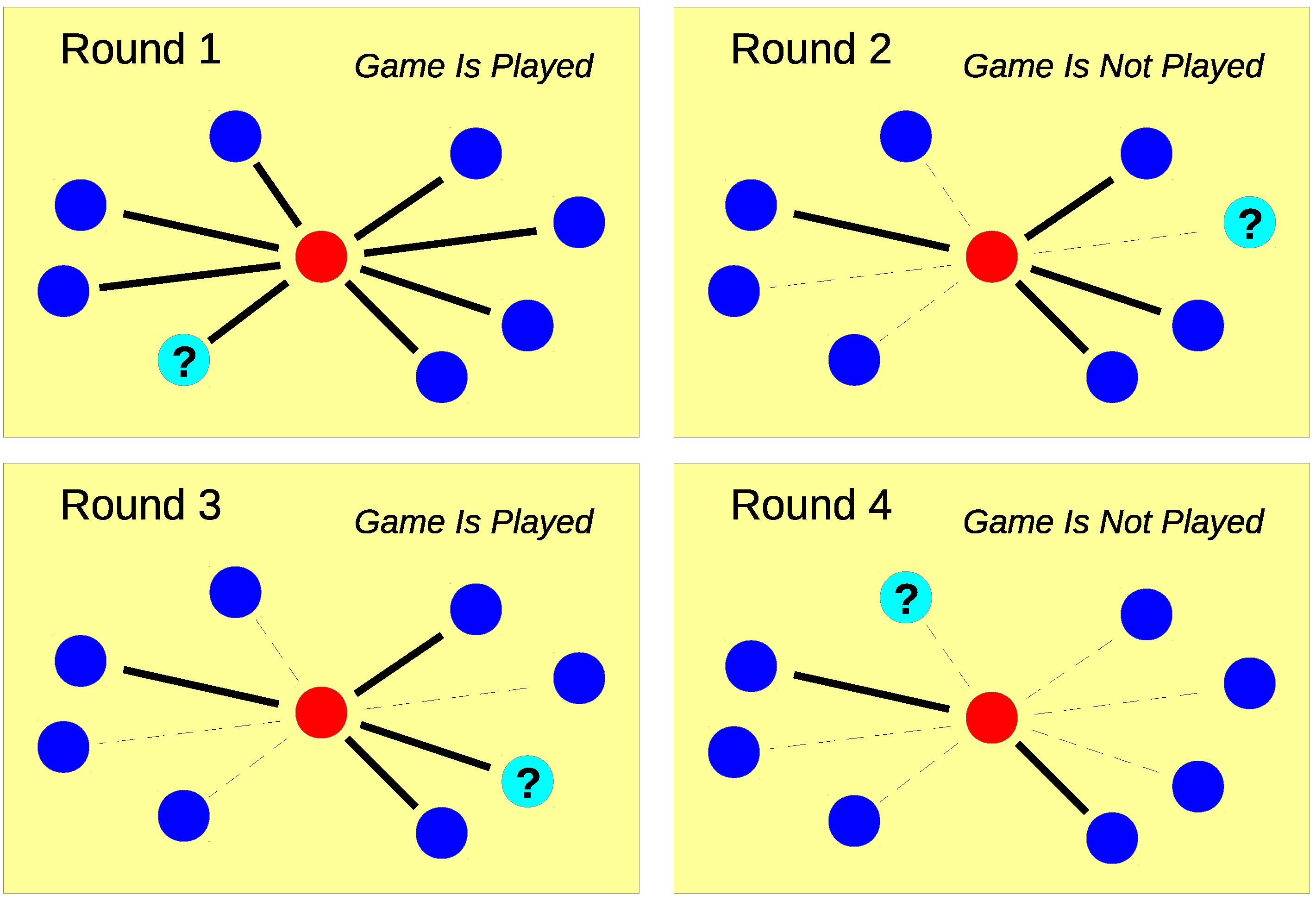
3.1. Single Defector

To make progress analytically, imagine the simpler case of a single defector in an infinitely large population of cooperators. In this simplified setting, the defector participates in m rounds and therefore is offered to play a game m times, each time with a random cooperator. (Note that in the dynamical model, M rounds are run in total between randomly selected pairs of individuals, but the number of rounds that a particular defector in the population participates in is a random variable. In the simplified static model, the sole defector participates in exactly m rounds.) After each exploitation of a cooperator, the exploited cooperator shares the identity of the solitary defector with each of the other uninformed cooperators with probability p = 1 - q . Thus, with probability q, each defector–cooperator link remains active after an exploitation of a cooperator by a defector. Informed cooperators always refuse a potential game with the defector. The fraction of cooperators in the population that are aware of the defector’s identity increases with the number of games played. Since informed cooperators always reject a game with the defector, cooperators can achieve a higher total payoff than the defector if many rounds are offered. A sample sequence of rounds is shown in Figure 1. Changes in the fraction of active links to cooperators as games are played are shown schematically in Figure 2.
Figure 1. Schematic illustrating indirect reciprocity with optional interactions and private information in a population with eight cooperators (blue) and a single defector (red). The population size is N = 9 . The defector is at the center of each image of the population. Each solid black line connecting the defector with a cooperator represents an active link. In the first round, the defector is offered a game with a random cooperator (light blue with a “?”), and the game is played. The defector gains payoff b. Each of the defector’s links is removed with probability p = 0 . 5 . After the first round, four of the defector’s links with cooperators are eliminated (thin dotted lines). In the second round, the defector is offered a game with a cooperator that knows the defector’s identity, so the potential game is rejected. In the third round, the defector again exploits an ignorant cooperator, and the defector again receives payoff b. Two of the remaining active links are eliminated. In the fourth round, the defector is offered a game with an informed cooperator, and the potential game is rejected. After this sequence of four rounds, the defector gains total payoff 2 b .
Games 06 00438 g001
Figure 2. Schematic showing how the fraction of active links between the defector and cooperators decreases as additional exploitations occur. At the start of a generation, all links to cooperators are active. On the first round, the defector plays a game, and a fraction q of the links remain active after the game. On each round thereafter, the defector plays another game with probability q i , where i is the number of games that have been played to that point.
Games 06 00438 g002
We denote the average number of games played in m rounds by a solitary defector in a population of infinitely many cooperators by F m ( q ) . We must find an expression for F m ( q ) . First, let us derive an expression for x i , m —the probability that the defector plays i games in m rounds. Suppose that the defector plays i times in m rounds. There are two possible cases: (i) the defector plays i times in the first m - 1 rounds and is rejected for play in round m; and (ii) the defector plays i - 1 times in the first m - 1 rounds and is accepted for play in round m. The probability for the first case is ( 1 - q i ) x i , m - 1 . The probability for the second case is q i - 1 x i - 1 , m - 1 . Therefore, the probability that the defector plays i times in m rounds is
x i , m = ( 1 - q i ) x i , m - 1 + q i - 1 x i - 1 , m - 1
This expression holds for any m i 2 with the convention that x m , m - 1 = 0 . For i = 1 , the second case does not occur and we have the recurrence formula
x 1 , m = ( 1 - q ) x 1 , m - 1 m 2
Since x 1 , 1 = 1 , we have
x 1 , m = ( 1 - q ) m - 1 m 1

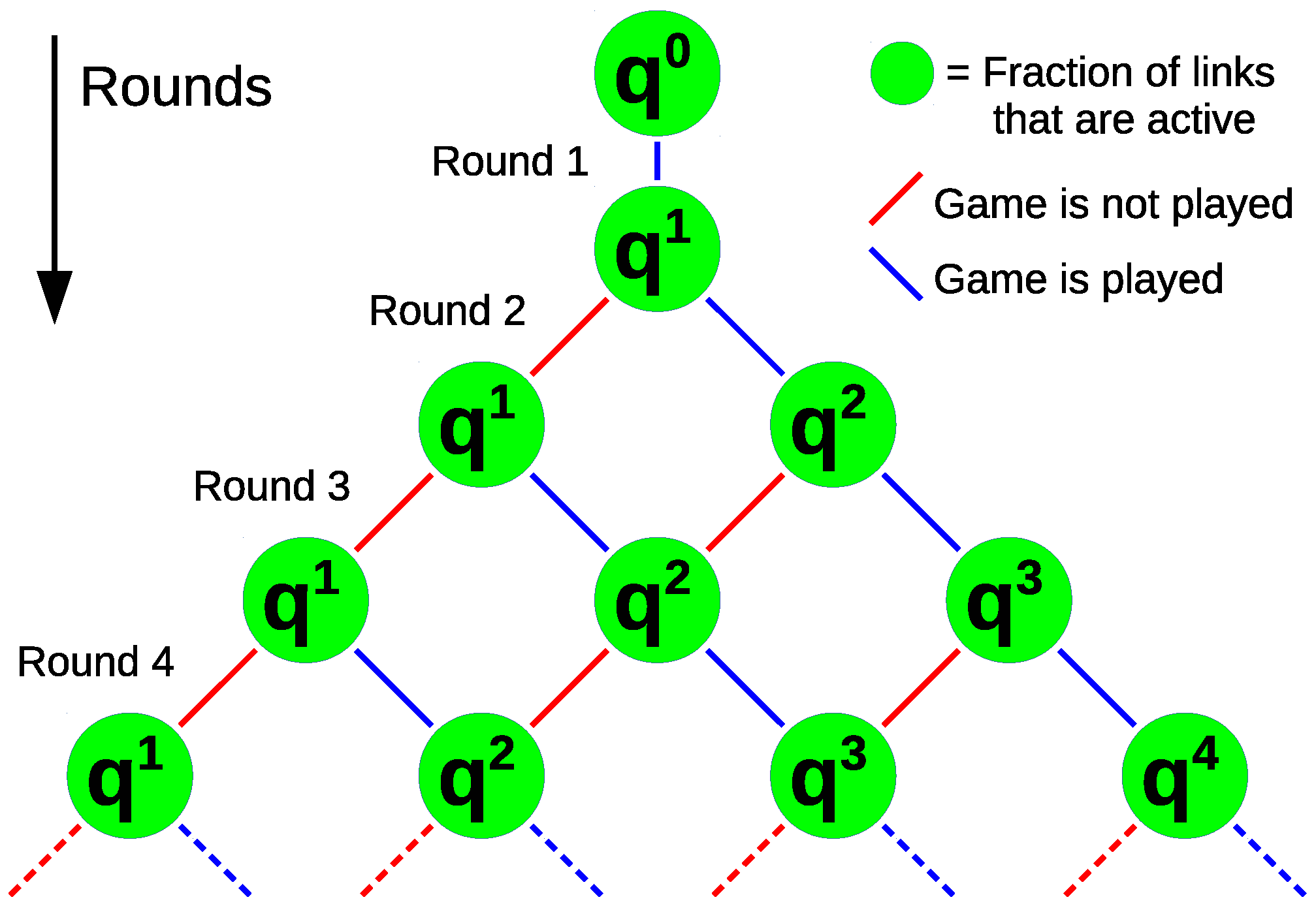
3.1.1. Probability of i Games in m Rounds

To solve the recurrence, Equation (1), for x i , m , it is helpful to first solve for its z-transform, which we write as
x ˜ i ( z ) = m = 0 z - m x i , m
From Equation (3) and Equation (2), the z-transform of x 1 , m is
x ˜ 1 ( z ) = 1 z m = 0 1 - q z m
We can consider the summation as a geometric series (with region of convergence | z | > 1 - q ), and we obtain
x ˜ 1 ( z ) = 1 z - ( 1 - q )
From Equation (3) and Equation (1), the z-transform of x i , m with i 2 is
x ˜ i ( z ) = ( 1 - q i ) z - 1 x ˜ i ( z ) + q i - 1 z - 1 x ˜ i - 1 ( z )
We see that x ˜ i ( z ) can be expressed recursively in terms of x ˜ i - 1 ( z ) :
x ˜ i ( z ) = q i - 1 z - ( 1 - q i ) x ˜ i - 1 ( z )
Iterating Equation (5) and substituting Equation (4), we find
x ˜ i ( z ) = n = 1 i q n - 1 z - ( 1 - q n )
Thus, the z-transformed quantity x ˜ i ( z ) has a simple, closed-form expression in terms of q, i, and z. All that remains is to invert the z-transform to obtain x i , m . Intuitively, Equation (6) has exactly i simple poles, and each simple pole corresponds to a separate term in the evaluation of x i , m . We have
x i , m = 1 2 π I C d z z m - 1 x ˜ i ( z ) = 1 2 π I C d z z m - 1 n = 1 i q n - 1 z - ( 1 - q n )
(I denotes the imaginary unit.) Here, C represents a counterclockwise closed contour encircling the origin and enclosing all poles of the integrand. For example, we can take a unit circle for C as all the zeros and poles have modulus less than 1. From the residue theorem, we have
x i , m = k = 1 i Res z = 1 - q k z m z n = 1 i q n - 1 z - ( 1 - q n )
We evaluate this as
x i , m = k = 1 i lim z 1 - q k [ z - ( 1 - q k ) ] z m z n = 1 i q n - 1 z - ( 1 - q n )
Simplifying Equation (7), we obtain
x i , m = k = 1 i ( - 1 ) i - k q i ( i - 1 ) / 2 ( 1 - q k ) m 1 - q k n = 1 k - 1 1 q n ( 1 - q n ) n = 1 i - k 1 q k ( 1 - q n )
This can be rearranged slightly as
x i , m = k = 1 i ( - 1 ) i - k q k + i ( i - 1 ) / 2 ( 1 - q k ) m n = 1 k 1 q n ( 1 - q n ) n = 1 i - k 1 q k ( 1 - q n )
Collecting factors of q, we have
x i , m = k = 1 i ( - 1 ) i - k q ( i - k ) ( i - k - 1 ) / 2 ( 1 - q k ) m n = 1 k 1 1 - q n n = 1 i - k 1 1 - q n
We make the substitution i = j + k . We also define
Q k = i = 1 k 1 1 - q i
Equation (8) can then be simplified as
x i , m = j = 0 i - 1 ( - 1 ) j q j ( j - 1 ) / 2 ( 1 - q i - j ) m Q i - j Q j
Equation (9) is proven using an alternative method in Appendix A.

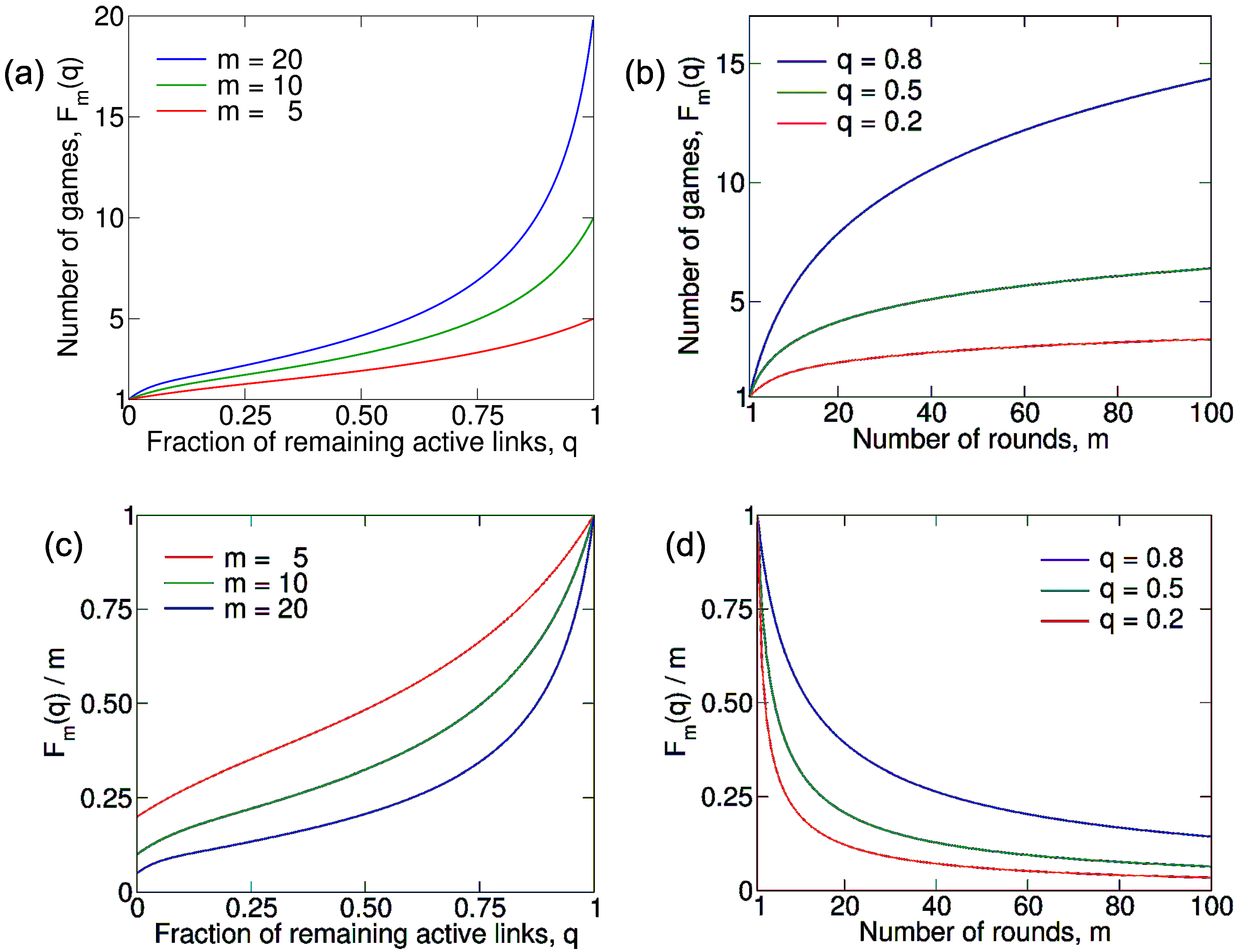
3.1.2. Average Number of Games

The average number of games played by the defector, F m ( q ) , is given by
F m ( q ) = i = 1 m i x i , m
From Equation (9) and Equation (10), and after rewriting the summations, we have
F m ( q ) = j = 1 m ( 1 - q j ) m Q j k = 0 m - j ( - 1 ) k ( j + k ) q k ( k - 1 ) / 2 Q k
In Figure 3, we plot Equation (11) in several ways.

3.2. Fixed Number of Rounds per Generation

More generally, consider that there are N C cooperators and N D defectors. Two players are selected randomly in each round and are offered a game. Each individual is selected, on average, m times in M total rounds. The total number of rounds, M, is a constant for each generation.

3.2.1. Average Number of Games

Define by f = N C / N the fraction of individuals in the population that are cooperators. A total of M rounds are run in each generation in a population of size N. Here, M can be expressed in terms of m (the average number of rounds that each individual engages in) as M = m N / 2 . The probability that a given defector engages in a particular round is 2 / N . In the limit N , the binomial distribution for the number of rounds that a given defector engages in becomes Poisson-distributed with expected value ( m N / 2 ) ( 2 / N ) = m . Moreover, the average number of times that a defector is selected for a possible game with a cooperator is f m , and this quantity is Poisson-distributed with expected value f m . Thus, we can write the average number of games played by a defector with cooperators in a generation as
G ( f , m ; p ) = e - f m k = 1 f k m k k ! F k ( 1 - p )
Here, p = 1 - q is the probability that a link between a cooperator and a defector is eliminated after the defector exploits a cooperator.
Figure 3. Average number of games that the defector plays. (a) Expected number of exploitations, F m ( q ) , against the probability, q, to maintain each link when m = 5 , 10, and 20 (bottom to top); (b) F m ( q ) against the number of rounds, m, when q = 0 . 2 , 0 . 5 , and 0 . 8 (bottom to top); (c) Expected number of exploitations normalized by the number of rounds, F m ( q ) / m , against the probability, q, to maintain each link when m = 5 , 10, and 20 (top to bottom); (d) F m ( q ) / m against the number of rounds, m, when q = 0 . 2 , 0 . 5 , and 0 . 8 (bottom to top).
Games 06 00438 g003

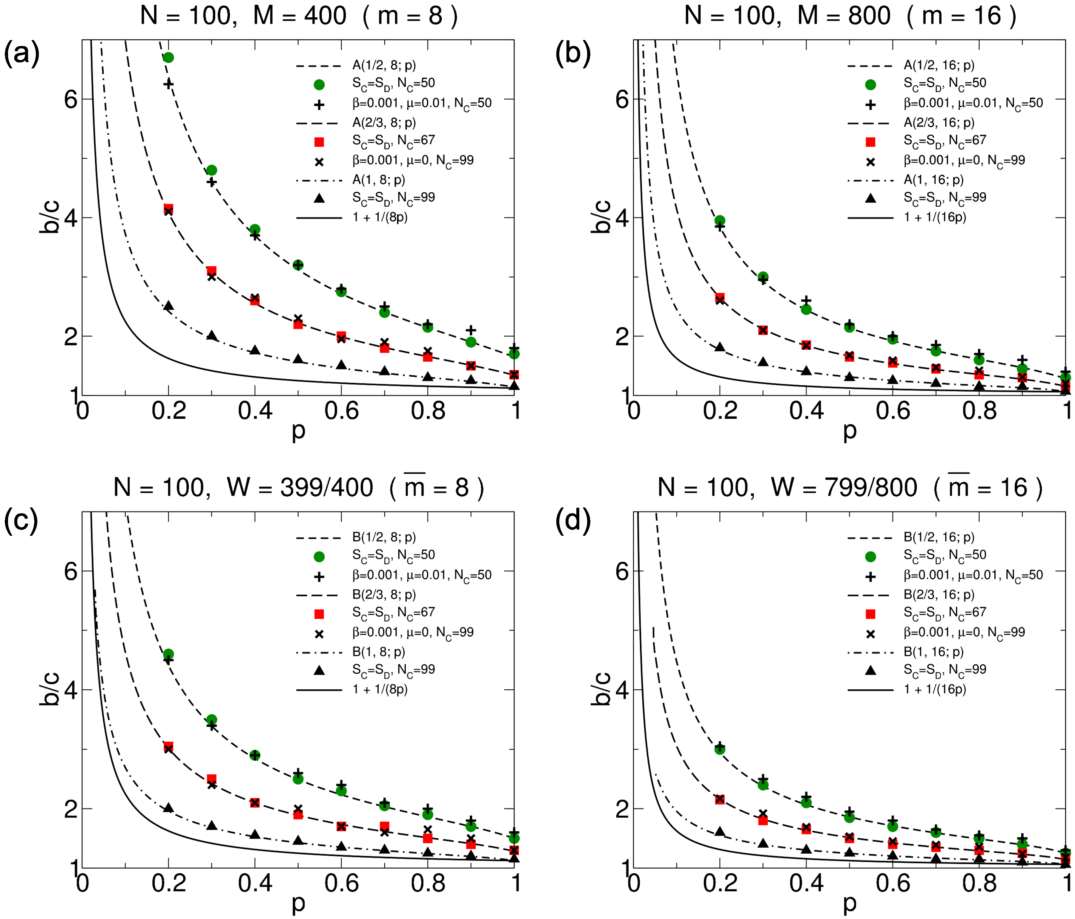
3.2.2. Critical Benefit-to-Cost Ratio

What is the critical benefit-to-cost ratio, b / c , needed to ensure that cooperators receive a higher payoff, on average, than defectors? We reason as follows: Each cooperator plays an average of f m games with other cooperators in a generation, so each cooperator receives a contribution to its payoff in the amount f m ( b - c ) . Each defector plays, on average, G ( f , m ; p ) games in a generation, so each defector receives average payoff b G ( f , m ; p ) . Each exploitation by a defector corresponds to a cost incurred by a cooperator without any compensating benefit. The total number of games that are played by defectors, on average, is N ( 1 - f ) G ( f , m ; p ) . Therefore, the average cost incurred by a cooperator due to exploitations by defectors is ( - c ) ( ( N ( 1 - f ) ) / ( N f ) ) G ( f , m ; p ) . Putting these pieces together, we find that the average cooperator payoff in a generation exceeds the average defector payoff in a generation if
f m ( b - c ) - c 1 - f f G ( f , m ; p ) > b G ( f , m ; p )
Rearranging Equation (12), we find that cooperators achieve a higher payoff that defectors, on average, if
b c > 1 + f f m G ( f , m ; p ) - 1 - 1 A ( f , m ; p )

3.2.3. Simulation Results

We next perform simulations for which the total number of rounds per generation, M, is fixed. The success of cooperation depends on the rate, p, at which information about the defectors is transferred among cooperators, on the fraction, f, of cooperators in the population, and on the average number of rounds per generation, m, that an individual engages in. We have that m = 2 M / N .
Simulation results for a fixed total number of rounds per generation are shown in Figure 4a,b. In Figure 4a, the total number of rounds per generation, M, is 400. Therefore, the average number of rounds per individual in a generation, m, is equal to 8. In Figure 4b, the total number of rounds per generation, M, is 800. Therefore, the average number of rounds per individual in a generation, m, is equal to 16.
We plot the critical value of b / c needed for cooperators to be more abundant than defectors with nonzero mutation rate, μ, and with weak intensity of selection, β (“+” symbols), for m = 8 and m = 16 . We also plot the critical value of b / c above which cooperators achieve a higher payoff in M total rounds, on average, than do defectors if f = 1 / 2 (green circles) for m = 8 and m = 16 . The two sets of data points agree well, as we would expect. In addition, we show the functions A ( 1 / 2 , 8 ; p ) and A ( 1 / 2 , 16 ; p ) . The agreement between theory and simulation is excellent.
In another measurement, we start with a single defector and allow the dynamics to progress with no mutation ( μ = 0 ) and with weak intensity of selection. We plot the critical value of b / c needed for the fixation probability at the all-defector state to be less than 1 / N (“X” symbols) for m = 8 and m = 16 when starting with a single defector. We also plot the critical value of b / c above which cooperators achieve a higher payoff in M total rounds, on average, than do defectors if f = 2 / 3 (red squares) for m = 8 and m = 16 . The two sets of data points agree well, as we would expect from the one-third law of evolutionary dynamics [2,47,48,49,50,51]. In addition, we show the functions A ( 2 / 3 , 8 ; p ) and A ( 2 / 3 , 16 ; p ) . The agreement between theory and simulation is again excellent.
In yet another measurement, we plot the critical value of b / c above which a solitary defector in a population of cooperators achieves a lower payoff in M total rounds, on average, than does a random cooperator (black triangles). This is the condition for cooperation to be a strict Nash equilibrium. We also show the functions A ( 1 , 8 ; p ) and A ( 1 , 16 ; p ) , again demonstrating outstanding agreement between theory and simulation.
Figure 4. The critical value of b / c for cooperation to be favored over defection in various settings. The green circles represent measured critical values of b / c for the average cooperator payoff to exceed the average defector payoff when f = 1 / 2 . The “+” symbols represent measured critical values of b / c for cooperators to outnumber defectors with weak selection and with weak mutation when their numbers are averaged over many successive generations. The red squares represent measured critical values of b / c for the average cooperator payoff to exceed the average defector payoff when f = 2 / 3 . The “×” symbols represent measured critical values of b / c for defectors to fix with probability less than 1 / N when starting with a single defector with weak selection and with no mutation. The black triangles represent measured critical values of b / c for the average cooperator payoff to exceed the average defector payoff when f = 1 (i.e., a single defector in a large population of cooperators). Panels (a,b) are for a fixed total number of rounds per generation, M, while panels (c,d) are for a variable total number of rounds per generation, M, where the average of M over generations is M ¯ = 1 / ( 1 - W ) . Error bars are roughly the size of the data points.
Games 06 00438 g004

3.3. Variable Number of Rounds per Generation

The only strict Nash equilibrium strategy and the only evolutionarily stable strategy in the classic prisoner’s dilemma with exactly m repeated interactions is to defect in every round [2,12,52]. In realistic settings, an individual may not know at the outset how many rounds it will participate in with potential interaction partners. It is therefore worthwhile to also consider a variable number of rounds per generation. In a variation of our dynamical model, we postulate that another round is run between two randomly chosen individuals with probability W. The average total number of rounds that are run is M ¯ = 1 / ( 1 - W ) . The average number of rounds that each defector engages in, averaged over generations, is m ¯ .

3.3.1. Average Number of Games

The probability that a total of M rounds are run is ( 1 - W ) W M - 1 . Analogously to G ( f , m ; p ) , we can write the average number of games played by a defector, H ( f , m ¯ ; p ) , as
H ( f , m ¯ ; p ) = lim N ( 1 - W ) M = 1 W M - 1 e - 2 f M N k = 1 2 k f k M k N k k ! F k ( 1 - p )
Intuitively, we are just multiplying the probability that a total of M rounds are offered in a generation with the average number of rounds offered to an individual, G ( f , m = 2 M / N ; p ) . We consider the limit of large population size, N , which is realistic and also admits simplified results. Denote the average number of rounds that an individual engages in by m ¯ . The value of W for which the average number of rounds engaged in per individual equals m ¯ is W = 1 - 2 / ( m ¯ N ) . We have
H ( f , m ¯ ; p ) = lim N 2 m ¯ N M = 1 1 - 2 m ¯ N M - 1 e - 2 f M N k = 1 2 k f k M k N k k ! F k ( 1 - p )
We can write this as
H ( f , m ¯ ; p ) = lim N 2 m ¯ N M = 1 1 - 2 m ¯ N m ¯ N 2 2 ( M - 1 ) m ¯ N e - 2 f M N k = 1 2 k f k M k N k k ! F k ( 1 - p )
In the limit of large population size, N , the factor in square brackets becomes e - 1 . Thus, we have
H ( f , m ¯ ; p ) = lim N 2 m ¯ N M = 1 e - 2 M m ¯ N e - 2 f M N k = 1 2 k f k M k N k k ! F k ( 1 - p )
This can be rewritten more suggestively as
H ( f , m ¯ ; p ) = 1 m ¯ lim N M = 1 2 Δ M N e - 1 + f m ¯ m ¯ 2 M N k = 1 f k k ! 2 M N k F k ( 1 - p )
Here, note that Δ M = 1 . (The summation increments M by 1 at each iteration.) Recall that m = 2 M / N . Since 2 Δ M / N = Δ m , we can consider Equation (14) as an integration over m. We have
H ( f , m ¯ ; p ) = 1 m ¯ 0 d m e - 1 + f m ¯ m ¯ m k = 1 f k k ! m k F k ( 1 - p )
Next, we define
ζ = 1 + f m ¯ m ¯ m
We have
H ( f , m ¯ ; p ) = 1 1 + f m ¯ k = 1 m ¯ 1 + f m ¯ k 0 d ζ e - ζ ζ k f k k ! F k ( 1 - p )
Notice that the integration over ζ is just Γ ( k + 1 ) = k ! . Thus, we have
H ( f , m ¯ ; p ) = 1 1 + f m ¯ k = 1 f m ¯ 1 + f m ¯ k F k ( 1 - p )

3.3.2. Critical Benefit-to-Cost Ratio

Analogously to Equation (12), the average cooperator payoff in a generation exceeds the average defector payoff in a generation if
f m ¯ ( b - c ) - c 1 - f f H ( f , m ¯ ; p ) > b H ( f , m ¯ ; p )
Rearranging Equation (15), we have
b c > 1 + f f m ¯ H ( f , m ¯ ; p ) - 1 - 1 B ( f , m ¯ ; p )

3.3.3. Simulation Results

We next perform simulations for which the total number of rounds per generation, M, is a random variable. The success of cooperation depends on the rate, p, at which information about the defectors is transferred among cooperators, on the fraction, f, of cooperators in the population, and on the average number of rounds per generation, m ¯ , that an individual engages in. The average number of rounds that an individual engages in during any single generation, m, is a random variable and is given by m = 2 M / N .
Simulation results for a variable total number of rounds per generation are shown in Figure 4c,d. In Figure 4c, the probability of another round, W, is 399 / 400 . Therefore, the average number of rounds per individual in a generation, m ¯ , is equal to 8. We plot B ( 1 / 2 , 8 ; p ) , B ( 2 / 3 , 8 ; p ) , and B ( 1 , 8 ; p ) . The agreement between theory and simulation is excellent. In Figure 4d, the probability of another round, W, is 799 / 800 . Therefore, the average number of rounds per individual in a generation, m ¯ , is equal to 16. We plot B ( 1 / 2 , 16 ; p ) , B ( 2 / 3 , 16 ; p ) , and B ( 1 , 16 ; p ) . The agreement between theory and simulation is again excellent.
Note the subtle distinction between the models investigated in Figure 4a,b and Figure 4c,d. In Figure 4a,b, the total number of rounds per generation is fixed and is equal to M, and the average number of rounds per individual in a generation is equal to m = 2 M / N . In Figure 4c,d, the probability of another round between two random individuals in a generation is equal to W. The total number of rounds per generation, M, for Figure 4c,d is therefore a random variable, with average given by M ¯ = 1 / ( 1 - W ) , and the average number of rounds per individual in a generation is equal to m ¯ = 2 M ¯ / N = 2 / ( N ( 1 - W ) ) . Notice that the critical values of b / c are lower in Figure 4c than in Figure 4a and are also lower in Figure 4d than in Figure 4b.

3.4. Simple Lower Bound on b / c

We now seek a simple condition on b / c for cooperation to be successful. Consider an individual in an infinitely large population of cooperators. The individual participates in m + 1 rounds with the infinite population of cooperators and has two choices of strategy: The focal individual may cooperate in all m + 1 rounds, receiving total payoff ( b - c ) ( m + 1 ) . Or the focal individual may defect on the first round but cooperate on all m subsequent rounds, receiving total payoff b + q m ( b - c ) . The strategy for the focal individual to always cooperate delivers a higher payoff after m + 1 rounds if
( b - c ) ( m + 1 ) > b + q m ( b - c )
We expect Equation (17) to yield a necessary condition on b / c for cooperation to be successful. Rearranging, we arrive at the condition
b c > 1 + 1 m p
If the total number of rounds, M, in a generation is a random variable, then we propose a variation of Equation (18):
b c > 1 + 1 m ¯ p
The simple condition, Equation (18), is plotted in Figure 4a,b (solid black curves). Notice that this form has the intuitively correct limiting behavior: The critical value of b / c increases as the rate of information transfer, p, decreases, and becomes infinite in the limit p 0 . The critical value of b / c decreases as the number of rounds, m, increases. As m , cooperators are able to accumulate an infinitely larger payoff than defectors in a single generation (provided that b - c > 0 ), and the critical value of b / c approaches 1. The simple condition, Equation (19), is also plotted in Figure 4c,d (solid black curves).

4. Discussion

We have studied a simple model for evolution of indirect reciprocity with private information. As information about the identity of defectors spreads among cooperators, defectors lose their fitness advantage. Interactions are optional; a cooperator can reject a possible game with a defector if it is cognizant of that defector’s identity. Thus, cooperation can eventually prevail.
We have derived exact conditions on the benefit-to-cost ratio for cooperation to dominate. We have also derived exact conditions on the benefit-to-cost ratio for natural selection to oppose the fixation of defectors starting with a single defector. Agreement of our theoretical predictions for either a fixed or a variable total number of rounds (Equation (13) and Equation (16), respectively) with simulation data is excellent. We have also deduced simple conditions on the benefit-to-cost ratio, Equation (18) and Equation (19), which ensure the success of cooperation.
Our calculations and simulations lend insight into indirect reciprocity with an evolving distribution of reputations. Increasing the rate of information transfer among cooperators and increasing the number of games offered to each individual in a generation both facilitate the transition to a population of cooperators. Intriguingly, the distribution of the total number of rounds in a generation significantly affects the critical benefit-to-cost ratio needed for cooperators to be favored. This is evident in Figure 4, where one sees that having a constant probability of another round in a generation (as opposed to having an exactly fixed total number of rounds per generation) is more favorable to cooperation.
Variations of our model are also possible. For example, a defector’s identity may be revealed in any round in which it is paired with a cooperator, even if the cooperator rejects the potential game. Notice that this modified model is significantly more conducive to the evolution of cooperation since information about defectors is transferred more rapidly. In this case, our critical benefit-to-cost ratios, Equation (13) and Equation (16), would represent sufficient conditions for cooperators to succeed. We derive results for the modified model in Appendix B.
In another variation, there is a cost for entering a game. In this case, even defectors would want to avoid playing with other defectors. It is now plausible that also defectors reveal the identities of other defectors that they have met. This modification also allows for easier evolution of cooperation, because the identity of defectors is revealed faster.
There are also possibilities for implementation errors. For example, when a cooperator engages in a round with a defector, the cooperator could mistake the defector for being another cooperator. Such recognition errors may involve new information transfer regarding the defector’s identity, which would reduce future exploitations of cooperators by that defector. Implementation errors could also result in erroneous information transfer if cooperators are mistakenly perceived as defectors. In this case, cooperators that are wrongly perceived as defectors might have their links with other cooperators severed for all subsequent rounds, which would make it more difficult for cooperators to thrive. However, a key point is that we endow cooperators with optional interactions. Therefore, on rare occasions, a cooperator might wrongfully view another cooperator as a defector and reject a potential game, but both individuals subsequently retain their strategies as cooperators. For this reason, we expect our derivations of critical benefit-to-cost ratios to be fairly robust provided that implementation errors are rare. Each of these modifications to our model is a potential topic for future study.

Acknowledgments

This publication was made possible through the support of a grant from the John Templeton Foundation (JO) and also through the support of a Samsung Scholarship (WG). The opinions expressed in this publication are those of the authors and do not necessarily reflect the views of the John Templeton Foundation and Samsung Scholarship.

Author Contributions

All authors performed research related to this work.

Conflicts of Interest

The authors declare no conflict of interest.

Appendix

A. Alternative Proof of the Formula for x i , m

We can alternatively prove Equation (9) for x i , m as follows. We begin by introducing the standard definition of q-analogue factorials:
[ n ] q ! = 1 ( 1 + q ) ( 1 + q + q 2 ) ( 1 + q + + q n - 1 )
The corresponding q-analogue binomial coefficients are
n k q = [ n ] q ! [ k ] q ! [ n - k ] q !
These quantities can be rewritten using the notation of Pochhammer symbols. We have
[ n ] q ! = ( q ; q ) n ( 1 - q ) n
and
n k q = ( q ; q ) n ( q ; q ) k ( q ; q ) n - k
Here, ( q ; q ) k is the kth q-Pochhammer symbol defined by
( q ; q ) k = i = 1 k ( 1 - q i )
From the well-known result for q-analogue binomials [45], we have
n k q = n - 1 k q + q n - k n - 1 k - 1 q
Using Equation (A1) and induction on n, we have the following result [46]:
( 1 + q x ) ( 1 + q 2 x ) ( 1 + q n x ) = j = 0 n q j + 1 2 n j q x j
By plugging x = - 1 / q n + 1 and x = - 1 / q k + 1 into Equation (A2), we have
j = 0 n ( - 1 ) j q j 2 n j q q ( n + 1 - j ) n = q n ( q n - 1 ) ( q n - q ) ( q n - q 2 ) ( q n - q n - 1 )
and
j = 0 n ( - 1 ) j q j 2 n j q q ( n + 1 - j ) k = 0 k = 0 , 1 , , n - 1
For any number α and positive integer n, we have the following identity:
j = 0 n ( - 1 ) j q j 2 n j q ( q n + 1 - j + α ) n = q n ( q n - 1 ) ( q n - q ) ( q n - q 2 ) ( q n - q n - 1 )
We obtain Equation (A5) by comparing the coefficients of α k using Equation (A3) and Equation (A4). Since both sides can be viewed as polynomials of α, it is enough to compare coefficients of α k for k = 0 , 1 , 2 , , n . The coefficient of α k for k = 1 , 2 , , n for the right hand side of Equation (A5) is zero. The coefficient of α k for k = 1 , 2 , , n for the left hand side of Equation (A5) is
j = 0 n ( - 1 ) j q j 2 n j q n k q ( n + 1 - j ) ( n - k ) = n k j = 0 n ( - 1 ) j q j 2 n j q q ( n + 1 - j ) ( n - k ) = 0
by Equation (A4). The constant term on the right hand side of Equation (A5) is q n ( q n - 1 ) ( q n - q ) ( q n - q 2 ) ( q n - q n - 1 ) . That of the left hand side of Equation (A5) is
j = 0 n ( - 1 ) j q j 2 n j q q ( n + 1 - j ) n = q n ( q n - 1 ) ( q n - q ) ( q n - q 2 ) ( q n - q n - 1 )
by Equation (A3). Thus, we have proven Equation (A5).
We can now present a formula for x i , m in terms of q-analogue factorials:
x i , m = j = 1 i ( - 1 ) i - j q i - j 2 ( 1 - q j ) m ( q ; q ) i - j ( q ; q ) j
We prove Equation (A6) by double induction on i and m. By direct computation, this holds for i = 1 and every m since x 1 , m = ( 1 - q ) m - 1 . Let us prove that this holds for i given that this holds for 1 , 2 , , i - 1 . For this step we use induction on m. Plugging n = i - 1 and α = - 1 into Equation (A5) and manipulating the indices, we have
j = 0 i - 1 ( - 1 ) j q j 2 i - 1 j q ( q i - j - 1 ) i - 1 = j = 1 i ( - 1 ) i - j q i - j 2 ( 1 - q j ) i ( q ; q ) i - j ( q ; q ) j = q i 2 = x i , i
Therefore, Equation (A6) satisfies Equation (1) when m = i . By direct computation, we can show that Equation (A6) satisfies Equation (1) for ( i , m ) given that it does for ( i , m - 1 ) :
x i , m - 1 = j = 1 i ( - 1 ) i - j q i - j 2 ( 1 - q j ) m ( q ; q ) i - j ( q ; q ) j 1 + 1 1 - q j - 1 = x i , m + q i j = 1 i ( - 1 ) i - j q i - j 2 ( 1 - q j ) m - 1 ( q ; q ) i - j ( q ; q ) j [ 1 + ( q j - i - 1 ) ] = x i , m + q i x i , m - 1 - q i - 1 j = 1 i - 1 ( - 1 ) i - 1 - j q i - 1 - j 2 ( 1 - q j ) m - 1 ( q ; q ) i - 1 - j ( q ; q ) j = x i , m + q i x i , m - 1 - q i - 1 x i - 1 , m - 1
Hence, we have the desired result.

B. Modification to the Model: Loss of Links on Every Round

Here, we consider a modification to our model in which there is information transfer every time a cooperator and a defector are paired. A fraction p of the defector’s remaining links with cooperators are broken on every round, even if the cooperator that is paired with the defector rejects the potential game. The formula analogous to Equation (1) for describing this modified model is
x i , m = ( 1 - q m - 1 ) x i , m - 1 + q m - 1 x i - 1 , m - 1
Here, x i , m is the probability of the solitary defector playing i games in m rounds when a fraction p of links are lost on every round. Equation (B1) holds for any m i 2 with the convention that x m , m - 1 = 0 . For i = 1 , we have the recurrence formula
x 1 , m = ( 1 - q m - 1 ) x 1 , m - 1 m 2
To solve Equation (B1), we introduce a z-transform on the index i:
x ˜ m ( z ) = i = 0 z - i x i , m
Notice that the only nonzero value of x i , m for m = 1 is x 1 , 1 = 1 . Using Equation (B2), we have
x ˜ 1 ( z ) = 1 z
From Equation (B2) and Equation (B1), the z-transform of x i , m with m 2 is
x ˜ m ( z ) = ( 1 - q m - 1 ) x ˜ m - 1 ( z ) + q m - 1 z - 1 x ˜ m - 1 ( z )
We see that x ˜ m ( z ) can be expressed recursively in terms of x ˜ m - 1 ( z ) :
x ˜ m ( z ) = ( 1 - q m - 1 ) z + q m - 1 z x ˜ m - 1 ( z )
Iterating Equation (B4) and substituting Equation (B3), we find
x ˜ m ( z ) = 1 z m n = 1 m ( 1 - q n - 1 ) z + q n - 1
From the above formula, we have the following by direct computation:
x i , m = 1 ( m - i ) ! d m - i d z m - i n = 1 m ( 1 - q n - 1 ) z + q n - 1 | z = 0
Equation (B5) can be simplified:
x i , m = I [ m - 1 ] and | I | = m - i k I ( 1 - q k ) k [ m - 1 ] I q k
We can compute the average number of games played by the defector by substituting Equation (B6) into Equation (10). In Figure B1, F m ( q ) / m is plotted for the original model and for the modified model. Notice that F m ( q ) is larger for the original model than for the modified model for all m 3 .
Figure B1. Average number of games that the defector plays in the original model (black curves) and the modified model (red curves). The expected number of exploitations normalized by the number of rounds, F m ( q ) / m , is plotted against the probability, q, to maintain each link when (a) m = 3 and (b) m = 4 . The inset in each panel shows the difference, Δ, between the black and red curves.
Games 06 00438 g005

References

  1. Nowak, M.A. Five rules for the evolution of cooperation. Science 2006, 314, 1560–1563. [Google Scholar] [CrossRef] [PubMed]
  2. Nowak, M.A. Evolutionary Dynamics; Harvard University Press: Cambridge, MA, USA, 2006. [Google Scholar]
  3. Bergstrom, T.C. Evolution of social behavior: Individual and group selection. J. Econ. Perspect. 2002, 16, 67–88. [Google Scholar] [CrossRef]
  4. Sasaki, T.; Uchida, S. The evolution of cooperation by social exclusion. Proc. R. Soc. Lond. B 2013, 280, 20122498. [Google Scholar] [CrossRef] [PubMed]
  5. Sugden, R. The Economics of Rights, Cooperation and Welfare; Basil Blackwell: Oxford, UK, 1986. [Google Scholar]
  6. Alexander, R.D. The Biology of Moral Systems; Aldine de Gruyter: New York, NY, USA, 1987. [Google Scholar]
  7. Kandori, M. Social norms and community enforcement. Rev. Econ. Stud. 1992, 59, 63–80. [Google Scholar] [CrossRef]
  8. Milinski, M.; Semmann, D.; Krambeck, H.-J. Reputation helps solve the “tragedy of the commons”. Nature 2002, 415, 424–426. [Google Scholar] [CrossRef] [PubMed]
  9. Rand, D.G.; Nowak, M.A. Human cooperation. Trends Cogn. Sci. 2013, 17, 413–425. [Google Scholar] [CrossRef] [PubMed]
  10. Yoeli, E.; Hoffman, M.; Rand, D.G.; Nowak, M.A. Powering up with indirect reciprocity in a large-scale field experiment. Proc. Natl. Acad. Sci. USA 2013, 110, 10424–10429. [Google Scholar] [CrossRef] [PubMed]
  11. Roberts, G. Evolution of direct and indirect reciprocity. Proc. R. Soc. Lond. B 2008, 275, 173–179. [Google Scholar] [CrossRef] [PubMed]
  12. Sigmund, K. The Calculus of Selfishness; Princeton University Press: Princeton, NJ, USA, 2010. [Google Scholar]
  13. Berger, U. Learning to cooperate via indirect reciprocity. Games Econ. Behav. 2011, 72, 30–37. [Google Scholar] [CrossRef] [Green Version]
  14. Wedekind, C.; Milinski, M. Cooperation through image scoring in humans. Science 2000, 288, 850–852. [Google Scholar] [CrossRef] [PubMed]
  15. Bolton, G.E.; Katok, E.; Ockenfels, A. Cooperation among strangers with limited information about reputation. J. Public Econ. 2005, 89, 1457–1468. [Google Scholar] [CrossRef]
  16. Semmann, D.; Krambeck, H.-J.; Milinski, M. Reputation is valuable within and outside one’s own social group. Behav. Ecol. Sociobiol. 2005, 57, 611–616. [Google Scholar] [CrossRef]
  17. Rockenbach, B.; Milinski, M. The efficient interaction of indirect reciprocity and costly punishment. Nature 2006, 444, 718–723. [Google Scholar] [CrossRef] [PubMed]
  18. Seinen, I.; Schram, A. Social status and group norms: indirect reciprocity in a repeated helping experiment. Eur. Econ. Rev. 2006, 50, 581–602. [Google Scholar] [CrossRef]
  19. Sommerfeld, R.D.; Krambeck, H.-J.; Semmann, D.; Milinski, M. Gossip as an alternative for direct observation in games of indirect reciprocity. Proc. Natl. Acad. Sci. USA 2007, 104, 17435–17440. [Google Scholar] [CrossRef] [PubMed]
  20. Ule, A.; Schram, A.; Riedl, A.; Cason, T.N. Indirect punishment and generosity toward strangers. Science 2009, 326, 1701–1704. [Google Scholar] [CrossRef] [PubMed]
  21. Jacquet, J.; Hauert, C.; Traulsen, A.; Milinski, M. Shame and honour drive cooperation. Biol. Lett. 2011, 7, 899–901. [Google Scholar] [CrossRef] [PubMed]
  22. Pfeiffer, T.; Tran, L.; Krumme, C.; Rand, D.G. The value of reputation. J. R. Soc. Interface 2012, 9, 2791–2797. [Google Scholar] [CrossRef] [PubMed]
  23. Leimar, O.; Hammerstein, P. Evolution of cooperation through indirect reciprocation. Proc. R. Soc. Lond. B 2001, 268, 745–753. [Google Scholar] [CrossRef] [PubMed]
  24. Ohtsuki, H.; Iwasa, Y. How should we define goodness? Reputation dynamics in indirect reciprocity. J. Theor. Biol. 2004, 231, 107–120. [Google Scholar] [CrossRef] [PubMed]
  25. Ohtsuki, H.; Iwasa, Y. The leading eight: Social norms that can maintain cooperation by indirect reciprocity. J. Theor. Biol. 2006, 239, 435–444. [Google Scholar] [CrossRef] [PubMed]
  26. Fishman, M.A. Indirect reciprocity among imperfect individuals. J. Theor. Biol. 2003, 225, 285–292. [Google Scholar] [CrossRef]
  27. Suzuki, S.; Akiyama, E. Evolution of indirect reciprocity in groups of various sizes and comparison with direct reciprocity. J. Theor. Biol. 2007, 245, 539–552. [Google Scholar] [CrossRef] [PubMed]
  28. Suzuki, S.; Akiyama, E. Three-person game facilitates indirect reciprocity under image scoring. J. Theor. Biol. 2007, 249, 93–100. [Google Scholar] [CrossRef] [PubMed] [Green Version]
  29. Martinez-Vaquero, L.A.; Cuesta, J.A. Evolutionary stability and resistance to cheating in an indirect reciprocity model based on reputation. Phys. Rev. E 2013, 87, 052810. [Google Scholar] [CrossRef]
  30. Suzuki, S.; Kimura, H. Indirect reciprocity is sensitive to costs of information transfer. Sci. Rep. 2013, 3. [Google Scholar] [CrossRef] [PubMed]
  31. Tanabe, S.; Suzuki, H.; Masuda, N. Indirect Reciprocity with Trinary Reputations. J. Theor. Biol. 2013, 317, 338–347. [Google Scholar] [CrossRef] [PubMed]
  32. Matsuo, T.; Jusup, M.; Iwasa, Y. The conflict of social norms may cause the collapse of cooperation: Indirect reciprocity with opposing attitudes towards in-group favoritism. J. Theor. Biol. 2014, 7, 34–46. [Google Scholar] [CrossRef] [PubMed]
  33. Brandt, H.; Sigmund, K. The logic of reprobation: Assessment and action rules for indirect reciprocation. J. Theor. Biol. 2004, 231, 475–486. [Google Scholar] [CrossRef] [PubMed]
  34. Brandt, H.; Sigmund, K. Indirect reciprocity, image scoring, and moral hazard. Proc. Natl. Acad. Sci. USA 2005, 102, 2666–2670. [Google Scholar] [CrossRef] [PubMed]
  35. Nowak, M.A.; Sigmund, K. Evolution of indirect reciprocity. Nature 2005, 427, 1291–1298. [Google Scholar] [CrossRef] [PubMed]
  36. Ohtsuki, H.; Iwasa, Y.; Nowak, M.A. Indirect reciprocity provides only a narrow margin of efficiency for costly punishment. Nature 2009, 457, 79–82. [Google Scholar] [CrossRef] [PubMed]
  37. Sigmund, K. Moral assessment in indirect reciprocity. J. Theor. Biol. 2012, 299, 25–30. [Google Scholar] [CrossRef] [PubMed]
  38. Nowak, M.A. Evolution of indirect reciprocity by image scoring. Nature 1998, 393, 573–577. [Google Scholar] [CrossRef] [PubMed]
  39. Nowak, M.A.; Sigmund, K. The dynamics of indrect reciprocity. J. Theor. Biol. 1998, 194, 561–574. [Google Scholar] [CrossRef] [PubMed]
  40. Uchida, S. Effect of private information on indirect reciprocity. Phys. Rev. E 2010, 82, 036111. [Google Scholar] [CrossRef]
  41. Uchida, S.; Sigmund, K. The competition of assessment rules for indirect reciprocity. J. Theor. Biol. 2010, 263, 13–19. [Google Scholar] [CrossRef] [PubMed]
  42. Nakamura, M.; Masuda, N. Indirect Reciprocity under Incomplete Observation. PLoS. Comput. Biol. 2011, 7, e1002113. [Google Scholar] [CrossRef] [PubMed]
  43. Uchida, S.; Sasaki, T. Effect of assessment error and private information on stern-judging in indirect reciprocity. Chaos Solitons Fractals 2013, 56, 175–180. [Google Scholar] [CrossRef]
  44. Ghang, W.; Nowak, M.A. Indirect reciprocity with optional interactions. J. Theor. Biol. 2015, 365, 1–11. [Google Scholar] [CrossRef] [PubMed]
  45. Van Lint, J.H.; Wilson, R.M. A Course in Combinatorics; Cambridge University Press: Cambridge, UK, 2001. [Google Scholar]
  46. Koekoek, R.; Swarttouw, R.F. The Askey-Scheme of Hypergeometric Orthogonal Polynomials and Its Q-Analogue; Faculty of Technical Mathematics and Informatics Report 98-17; Technische Universiteit Delft: Delft, The Netherlands, 1998; p. 7. [Google Scholar]
  47. Ohtsuki, H.; Bordalo, P.; Nowak, M.A. The one-third law of evolutionary dynamics. J. Theor. Biol. 2007, 249, 289–295. [Google Scholar] [CrossRef] [PubMed]
  48. Nowak, M.A.; Sasaki, A.; Taylor, C.; Fudenberg, D. Emergence of cooperation and evolutionary stability in finite populations. Nature 2004, 428, 646–650. [Google Scholar] [CrossRef] [PubMed]
  49. Imhof, L.A.; Nowak, M.A. Evolutionary game dynamics in a Wright-Fisher process. J. Math. Biol. 2006, 52, 667–681. [Google Scholar] [CrossRef]
  50. Lessard, S.; Ladret, V. The probability of fixation of a single mutant in an exchangeable selection model. J. Math. Biol. 2007, 54, 721–744. [Google Scholar] [CrossRef] [PubMed]
  51. Ladret, V.; Lessard, S. Evolutionary game dynamics in a finite asymmetric two-deme population and emergence of cooperation. J. Theor. Biol. 2008, 255, 137–151. [Google Scholar] [CrossRef] [PubMed]
  52. Brandt, H.; Sigmund, K. The good, the bad and the discriminator—Errors in direct and indirect reciprocity. J. Theor. Biol. 2006, 239, 183–194. [Google Scholar] [CrossRef] [PubMed]

