Strong Migration Limit for Games in Structured Populations: Applications to Dominance Hierarchy and Set Structure

Abstract

In this paper, we deduce a condition for a strategy $S_1$ to be more abundant on average at equilibrium under weak selection than another strategy $S_2$ in a population structured into a finite number of colonies of fixed proportions as the population size tends to infinity. It is assumed that one individual reproduces at a time with some probability depending on the payoff received in pairwise interactions within colonies and between colonies and that the offspring replaces one individual chosen at random in the colony into which the offspring migrates. It is shown that an expected weighted average equilibrium frequency of $S_1$ under weak symmetric strategy mutation between $S_1$ and $S_2$ is increased by weak selection if an expected weighted payoff of $S_1$ near neutrality exceeds the corresponding expected weighted payoff of $S_2$. The weights are given in terms of reproductive values of individuals in the different colonies in the neutral model. This condition for $S_1$ to be favoured by weak selection is obtained from a strong migration limit of the genealogical process under neutrality for a sample of individuals, which is proven using a two-time scale argument. The condition is applied to games between individuals in colonies with linear or cyclic dominance and between individuals belonging to groups represented by subsets of a given set.

1. Introduction

Population structure refers to consistent demographic differences among individuals as a function of some other attribute, such as geographic location, age, size, gender or physiological state. Over the last few years, structured population models have become a central modelling formalism in theoretical biology and game dynamics, as well as being one of the most widely used.

An important question is the effect of migration on evolution. Nagylaki [1] studied the strong migration limit in a geographically-structured population, which occurs when migration dominates all other evolutionary forces in the limit of a large population, by means of a diffusion approximation. He considers a finite number of demes represented by the integers $1,\dots ,d$. Deme i is composed of $N_i=N{\alpha }_i$ diploid individuals considered at a single multi-allelic locus, for $i=1,\dots ,d$. Here, N and ${\alpha }_i$ denote the whole population size and the proportion of deme i in the whole population, for $i=1,\dots ,d$, with ${\sum }_{i=1}^d{\alpha }_i=1$. Time is discrete with non-overlapping generations, and the reproduction scheme in each deme follows the Wright–Fisher model as a result of random mating. Following the production of a very large number of offspring and selection among offspring, there is migration. The probability that an individual in deme i comes from deme j is represented by $m_{ij}^{*}$, for $i,j=1,\dots ,d$. The backward migration matrix ${\mathbf{M}}^{*}={\left(m_{ij}^{*}\right)}_{1\le i,j\le d}$ is assumed to be constant and ergodic. Following migration and mutation, there is random sampling within demes to restore the deme sizes. In the limit of a large population size ($N\to \infty$), the stochastic dynamics in this structured population is described by a Wright–Fisher diffusion as in a well-mixed population with an effective population size $N_e=\alpha N$ taken as the unit of time, where:

$$\alpha ={\left(\sum _{i=1}^d\frac{{\pi }_i^2}{{\alpha }_i}\right)}^{-1}$$

(1)

Here, ${\left({\pi }_i\right)}_{1\le i\le d}$ is the stationary distribution associated with the backward migration matrix ${\mathbf{M}}^{*}$. Under the same assumptions, but for a haploid population and in the absence of selection, Notohara [2] showed that the genealogical process, known in this context as the structured coalescent (Herbots [3]), is described in the limit of a large population size by the standard Kingman coalescent [4,5,6], which is such that each pair of lineages coalesces backward in time at rate one independently of all others.

Diffusion approximations and genealogical processes are very important tools to address questions related to the effect of selection on the evolution of strategies in game dynamics. Among these questions, how cooperation can emerge and persist from interactions between individuals is of prime interest. This question has attracted increasing attention from mathematical or theoretical biologists (Axelrod and Hamilton [7], Szabò and Töke [8], Traulsen et al. [9], Santos and Pacheco [10], Hauert and Szabò [11], Nowak [12,13], Nowak and Sigmund [14], Ohtsuki et al. [15], Szabò and Fáth [16]). In order to study this question, a simple game named the prisoner’s dilemma has been considered. The simplest form of this game has payoffs in additive form with the following parameters: a donor pays a cost c to a recipient to get a benefit b, where $b>c$.

The first studies on the evolution of cooperation in structured populations assumed symmetric interactions between all members of the population. This means that the payoffs depend only on the strategies used by the interacting individuals (Hamilton [17,18], Trivers [19], Frank [20], Nowak and Sigmund [21,22], Nowak [23], Traulsen and Nowak [24], Kroumi and Lessard [25]). Even in this case, interactions can form a complex system as in the set-structured population introduced in Tarnita et al. [26]: every individual of the population belongs to exactly K sets among M sets, and a cooperator cooperates only with individuals that belong to at least L of the K sets, and defects otherwise.

In living groups, repetitive interactions for access to limited resources or mating opportunities can lead to the creation of a social order. A hierarchy dominance that may depend on differences in resource holding power (Hammerstein [27], Wilson [28]) can be established so that individuals are dominant over those below them and submissive to those above them. This motivates the study of asymmetric interactions with a cost for not conforming to the established hierarchy in structured populations with linear or cyclic dominance (Tao et al. [29], Kroumi and Lessard [30]).

In this paper, we consider a Moran-type model for games played in a population structured into d colonies of different finite sizes. In pairwise interactions, the individuals can adopt one of two strategies, $S_1$ or $S_2$. An individual from colony i interacts with an individual from colony j with probability $q_{ij}$ for $i,j=1,\dots ,d$, where ${\sum }_{j=1}^d{q}_{ij}=1$ for $i=1,\dots ,d$. The expected payoff that an individual receives determines the probability for this individual to produce an offspring. One offspring is produced at a time, and following migration, this offspring replaces one individual locally chosen at random. More precisely, if the offspring is produced in colony i and migrates to colony j with probability $m_{ij}$, then the offspring replaces an individual chosen at random in colony j, for $i,j=1,\dots ,d$. Finally, there is mutation of the strategy used by each individual independently of all others with probability u from one time step to the next, and when this occurs, the mutant strategy is chosen at random among $S_1$ and $S_2$. We will find a condition for $S_1$ to be more abundant on average than $S_2$ at equilibrium in the limit of a large population under weak selection and weak mutation. This result relies on the strong migration limit of the genealogical process in the absence of selection, which is proven using a lemma for two-time scale Markov chains due to Möhle [31]. The condition will be express in terms of expected weighted payoffs using reproductive values as weights, which is an alternative to the use of structure coefficients (Nowak et al. [32]) for games in structured populations. This will allow us to give an intuitive interpretation of this condition.

The remainder of this paper is organized as follows. We present the details of the model in Section 2. We use a two-time scale convergence result that is established in Appendix A to derive the limiting genealogical process in a neutral structured population in Section 3. The equilibrium state under weak selection is studied in Section 4. In Section 5, a condition for a weighted average equilibrium frequency of $S_1$ to increase as the selection intensity increases from zero is deduced. This condition is applied to situations with linear or cyclic dominance hierarchy in Section 6 and to games in set-structured populations in Section 7. The results are interpreted and discussed in Section 8.

2. Model

We assume a population subdivided into d colonies represented by the integers $1,\dots ,d$. Each colony is made of a finite number $N_i$ of haploid individuals, for $i=1,\dots ,d$. Each individual in the population adopts one of two strategies, $S_1$ or $S_2$. We assume pairwise interactions between individuals within each colony and between individuals from different colonies. More precisely, an individual from colony i interacts with an individual chosen at random from colony j with probability $q_{ij}$, for $j=1,\dots ,d$, with ${\sum }_{j=1}^d{q}_{ij}=1$, for $i=1,\dots ,d$. Then, the payoff that the individual from i receives is given by the entries of the matrix:

$${\mathbf{A}}_{ij}=\begin{array}{cc}& \begin{array}{cc}{S}_1& S_2\end{array}\\ \begin{array}{c}\begin{array}{c}{S}_1\\ S_2\end{array}\end{array}& \begin{array}{c}(& \begin{array}{cc}{a}_{ij}& b_{ij}\\ c_{ij}& d_{ij}\end{array}& )\end{array}\end{array}$$

(2)

according to the strategy adopted by the individual from i, corresponding to row $S_1$ or $S_2$, and the strategy used by the individual from j, corresponding to column $S_1$ or $S_2$. The expected payoffs of strategies $S_1$ and $S_2$ played by individuals in colony i are denoted by ${\phi }_{1,i}$ and ${\phi }_{2,i}$, respectively. It is assumed that these expected payoffs translate into fertilities, or reproductive successes, in the form:

$$f_{1,i}=1+s\times {\phi }_{1,i}$$

(3)

and:

$$f_{2,i}=1+s\times {\phi }_{2,i}$$

(4)

respectively, where $s>0$ represents the intensity of selection. It is assumed throughout the paper that selection is weak, actually that the intensity of selection s is small compared to the inverse of the population size $N^{-1}$, where:

$$N=N_1+\cdots +N_d$$

(5)

The case $s=0$ corresponds to neutrality.

Time is discrete. At each time step, an individual is chosen in the whole population with probability proportional to its fertility to produce an offspring. This offspring inherits the strategy used by its parent. If the parent is from colony i, then the offspring stays in colony i with probability $m_{ii}$ or migrates to colony $j\ne i$ with probability $m_{ij}$, with ${\sum }_{j=1}^d{m}_{ij}=1$, for $i=1,\dots ,d$. In both cases, the offspring replaces an individual chosen at random in the same colony. It is assumed throughout that the forward migration matrix $\mathbf{M}={\left(m_{ij}\right)}_{1\le i,j\le d}$ is irreducible and aperiodic, that is ergodic. In other words, there exists some power of this migration matrix, ${\mathbf{M}}^k$ for some integer $k\ge 1$, with all positive entries. Finally, strategy mutation occurs with probability u for each individual independently of all others, so that the strategy used by the individual at the next time step is chosen at random among $S_1$ and $S_2$ with probability u and remains the same with the complementary probability $1-u$.

3. Genealogical Process in the Neutral Model

In this section, we derive the genealogical process of a sample taken from the population structured into d colonies under the neutral model in the limit of a large population size. Every individual of the population has the same fertility, which is given by one.

Consider a sample of size $n\ge 2$ at a given time step. Looking backward in time at the genealogy of this sample, the distribution of the ancestors in the d colonies at any previous time step can be described by a vector:

$$\mathbf{n}=(n_1,\dots ,n_d)$$

(6)

where $n_i$ denotes the number of ancestors in colony i, for $i=1,\dots ,d$. Then:

$$\left|\mathbf{n}\right|=n_1+\cdots +n_d$$

(7)

is the total number of ancestors.

Let $\mathbf{n}(\tau )$ be the distribution of the ancestors $\tau \ge 0$ time steps back. Given an initial sample of n individuals, this is a discrete-time Markov chain with state space:

$$E_n=\left\{\mathbf{n}=(n_1,\dots ,n_d):n_1+\cdots +n_d\le n\right\}$$

(8)

Let ${\Pi }_{\mathbf{n},{\mathbf{n}}^{\prime }}$ be the transition probability from state $\mathbf{n}$ to state ${\mathbf{n}}^{\prime }$. A possible transition is from $\mathbf{n}$ to $\mathbf{n}-{\mathbf{e}}_i$, for $i\in \{1,\dots ,d\}$, such that $n_i\ge 1$. Here, ${\mathbf{e}}_i$ is a d-dimensional unit vector with the i-th component equal to one and all other components equal to zero. This transition is obtained if one of the $n_i$ ancestors in colony i produced an offspring who stayed in colony i and is one of the $n_i-1$ other ancestors in this colony, or if one of the $n_j$ ancestors in colony $j\ne i$ produced an offspring who migrated to colony i and is one of the $n_i$ ancestors in this colony. All this occurs with probability:

$${\Pi }_{\mathbf{n},\mathbf{n}-{\mathbf{e}}_i}=\frac{n_i}{N}{m}_{ii}\frac{(n_i-1)}{N_i}+\sum _{j\ne i}\frac{n_j}{N}{m}_{ji}\frac{n_i}{N_i}=\left(\frac{n_i(n_i-1)}{{\alpha }_i}{m}_{ii}+\sum _{j\ne i}\frac{n_i{n}_j}{{\alpha }_i}{m}_{ji}\right)\times \frac{1}{N^2}$$

(9)

Here, ${\alpha }_i=N_i/N$ is the proportion of colony i in the whole population, for $i=1,\dots ,d$. Another possible transition is from $\mathbf{n}$ to $\mathbf{n}-{\mathbf{e}}_i+{\mathbf{e}}_j$, for $i,j\in \{1,\dots ,d\}$, such that $n_i\ge 1$ and $i\ne j$. This occurs if an individual in colony j other than the $n_j$ ancestors in this colony produced an offspring who migrated to colony i and is one of the $n_i$ ancestors in this colony. The probability of this event is:

$${\Pi }_{\mathbf{n},\mathbf{n}-{\mathbf{e}}_i+{\mathbf{e}}_j}=\frac{(N_j-n_j)}{N}{m}_{ji}\frac{n_i}{N_i}=\frac{n_i{\alpha }_j}{{\alpha }_i}{m}_{ji}\times \frac{1}{N}-\frac{n_i{n}_j}{{\alpha }_i}{m}_{ji}\times \frac{1}{N^2}$$

(10)

The last transition with positive probability is to stay in the same state, for which we have:

$$\begin{array}{cc}\hfill {\Pi }_{\mathbf{n},\mathbf{n}}& =1-\sum _{i:n_i\ge 1}{\Pi }_{\mathbf{n},\mathbf{n}-{\mathbf{e}}_i}-\sum _{{}_{n_i\ge 1}^{i\ne j}}{\Pi }_{\mathbf{n},\mathbf{n}-{\mathbf{e}}_i+{\mathbf{e}}_j}\hfill \end{array}$$

$$\begin{array}{cc}& =1-\left(\sum _{{}_{n_i\ge 1}^{i\ne j:}}\frac{n_i{\alpha }_j}{{\alpha }_i}{m}_{ji}\right)\times \frac{1}{N}-\left(\sum _{i:n_i\ge 1}\frac{n_i(n_i-1)}{{\alpha }_i}{m}_{ii}\right)\times \frac{1}{N^2}\hfill \end{array}$$

(11)

From Equations (9)–(11), the transition matrix ${\Pi }_N={\left({\Pi }_{\mathbf{n},{\mathbf{n}}^{\prime }}\right)}_{\mathbf{n},{\mathbf{n}}^{\prime }\in E_n}$ can be decomposed into the form:

$${\Pi }_N=\mathbf{I}+\frac{\mathbf{A}}{N}+\frac{\mathbf{B}}{N^2}$$

(12)

Here, $\mathbf{I}$ is an identity matrix of a size given by the number of elements in the state space $E_n$, and $\mathbf{A}={\left(a_{\mathbf{n},{\mathbf{n}}^{\prime }}\right)}_{\mathbf{n},{\mathbf{n}}^{\prime }\in E_n}$ is an infinitesimal generator whose non-null entries are given by:

$$a_{\mathbf{n},{\mathbf{n}}^{\prime }}=\left\{\begin{array}{cc}\frac{n_i{\alpha }_j}{{\alpha }_i}{m}_{ji}\hfill & \text{if}{\mathbf{n}}^{\prime }=\mathbf{n}-{\mathbf{e}}_i+{\mathbf{e}}_j,\text{for}i\ne j\text{and}{n}_i\ge 1\hfill \\ -\sum _{{}_{n_i\ge 1}^{i\ne j:}}\frac{n_i{\alpha }_j}{{\alpha }_i}{m}_{ji}\hfill & \text{if}{\mathbf{n}}^{\prime }=\mathbf{n}\hfill \end{array}\right.$$

(13)

Moreover, the non-null entries of $\mathbf{B}={\left(b_{\mathbf{n},{\mathbf{n}}^{\prime }}\right)}_{\mathbf{n},{\mathbf{n}}^{\prime }\in E_n}$ are given by:

$$b_{\mathbf{n},{\mathbf{n}}^{\prime }}=\left\{\begin{array}{cc}\frac{n_i(n_i-1)}{{\alpha }_i}{m}_{ii}+\sum _{j\ne i}\frac{n_i{n}_j}{{\alpha }_i}{m}_{ji}\hfill & \text{if}{\mathbf{n}}^{\prime }=\mathbf{n}-{\mathbf{e}}_i,\text{for}i\text{such}\text{that}{n}_i\ge 1\hfill \\ -\frac{n_i{n}_j}{{\alpha }_i}{m}_{ji}\hfill & \text{if}{\mathbf{n}}^{\prime }=\mathbf{n}-{\mathbf{e}}_i+{\mathbf{e}}_j,\text{for}i\ne j\text{and}{n}_i\ge 1\hfill \\ -\sum _{i:n_i\ge 1}\frac{n_i(n_i-1)}{{\alpha }_i}{m}_{ii}\hfill & \text{if}{\mathbf{n}}^{\prime }=\mathbf{n}\hfill \end{array}\right.$$

(14)

Now, let ${\Gamma }_k$ be the subset of all possible states with k ancestors, namely:

$${\Gamma }_k=\{\mathbf{n}=(n_1,\dots ,n_d):\left|\mathbf{n}\right|=n_1+\cdots +n_d=k\}$$

(15)

for $k=1,\dots ,n$. Note that the set $E_n$ is the disjoint union of the subsets ${\Gamma }_1$, ${\Gamma }_2$, $\dots ,{\Gamma }_n$. With respect to these subsets in this order, the matrices $\mathbf{A}$ and $\mathbf{B}$ whose non-null entries $a_{\mathbf{n},{\mathbf{n}}^{\prime }}$ and $b_{\mathbf{n},{\mathbf{n}}^{\prime }}$ are given by Equations (13) and (14), respectively, can be expressed in the block forms:

$$\mathbf{A}=\left(\begin{array}{cccc}{\mathbf{A}}_1& \mathbf{0}& \dots & \mathbf{0}\\ \mathbf{0}& {\mathbf{A}}_2& \dots & \mathbf{0}\\ ⋮& ⋮& \ddots & ⋮\\ \mathbf{0}& \mathbf{0}& \dots & {\mathbf{A}}_n\end{array}\right)$$

(16)

and:

$$\mathbf{B}=\left(\begin{array}{cccccc}\mathbf{0}& \mathbf{0}& \mathbf{0}& \dots & \mathbf{0}& \mathbf{0}\\ {\mathbf{B}}_{2,1}& {\mathbf{B}}_{2,2}& \mathbf{0}& \dots & \mathbf{0}& \mathbf{0}\\ \mathbf{0}& {\mathbf{B}}_{3,2}& {\mathbf{B}}_{3,3}& \dots & \mathbf{0}& \mathbf{0}\\ ⋮& ⋮& ⋮& \ddots & ⋮& ⋮\\ \mathbf{0}& \mathbf{0}& \mathbf{0}& \dots & {\mathbf{B}}_{n,n-1}& {\mathbf{B}}_{n,n}\end{array}\right)$$

(17)

Here, $\mathbf{0}$ denotes a zero matrix of any dimension.

The exponential matrix $exp\left\{m\mathbf{A}\right\}$ for every integer $m\ge 1$ takes the block form:

$$exp\left\{m\mathbf{A}\right\}=\left(\begin{array}{cccc}exp\left\{m{\mathbf{A}}_1\right\}& \mathbf{0}& \dots & \mathbf{0}\\ \mathbf{0}& exp\left\{m{\mathbf{A}}_2\right\}& \dots & \mathbf{0}\\ ⋮& ⋮& \ddots & ⋮\\ \mathbf{0}& \mathbf{0}& \dots & exp\left\{m{\mathbf{A}}_n\right\}\end{array}\right)$$

(18)

Note that ${\mathbf{A}}_k$ is the infinitesimal generator of an irreducible Markov chain on a finite state space, which is ${\Gamma }_k$, for $k=1,\dots ,n$. Consequently, the limit matrix:

$${\mathbf{P}}_k:=\underset{m\to \infty }{lim}exp\left\{m{\mathbf{A}}_k\right\}$$

(19)

exists for $k=1,\dots ,n$, and so does:

$$\mathbf{P}:=\underset{m\to \infty }{lim}exp\left\{m\mathbf{A}\right\}=\left(\begin{array}{cccc}{\mathbf{P}}_1& \mathbf{0}& \dots & \mathbf{0}\\ \mathbf{0}& {\mathbf{P}}_2& \dots & \mathbf{0}\\ ⋮& ⋮& \ddots & ⋮\\ \mathbf{0}& \mathbf{0}& \dots & {\mathbf{P}}_n\end{array}\right)$$

(20)

Note also that ${\mathbf{P}}_k$ is actually a rank one matrix with the stationary distribution associated with ${\mathbf{A}}_k$ in every row, for $k=1,\dots ,n$. It remains to find this distribution.

Let $({\pi }_1,\dots ,{\pi }_d)$ be the stationary distribution associated with ${\mathbf{A}}_1$. By definition, this distribution satisfies the equation:

$$({\pi }_1,\dots ,{\pi }_d){\mathbf{A}}_1=(0,\dots ,0)$$

(21)

with:

$${\pi }_1+\cdots +{\pi }_d=1$$

(22)

Note that ${\mathbf{A}}_1=N({\mathbf{M}}^{*}-\mathbf{I})$, where ${\mathbf{M}}^{*}={\left(m_{ij}^{*}\right)}_{1\le i,j\le d}$ is the backward migration matrix, whose entries are given by:

$$m_{ij}^{*}=\left\{\begin{array}{cc}\frac{m_{ji}{N}_j}{N{N}_i}\hfill & \text{if}i\ne j\hfill \\ 1-\sum _{l\ne i}\frac{m_{li}{N}_l}{N{N}_i}\hfill & \text{if}i=j\hfill \end{array}\right.$$

(23)

This is obtained from Equation (13) in the case where $\mathbf{n}={\mathbf{e}}_i$ for $i=1,\dots ,d$. The entry $m_{ij}^{*}$ is the probability that an individual chosen at random in colony i comes from colony j one time step back. Moreover,

$$({\pi }_1,\dots ,{\pi }_d){\mathbf{M}}^{*}=({\pi }_1,\dots ,{\pi }_d)$$

(24)

which means that $({\pi }_1,\dots ,{\pi }_d)$ is the stationary distribution associated with the backward migration matrix ${\mathbf{M}}^{*}$. The stationary distribution associated with ${\mathbf{A}}_k$, for $k=2,\dots ,n$, can be expressed with respect to this distribution. For $\mathbf{n}=(n_1,\dots ,n_d)\in {\Gamma }_k$, we have:

$${\pi }_{\mathbf{n}}=\left(\genfrac{}{}{0pt}{}{\left|\mathbf{n}\right|}{n_1,n_2,\dots ,n_d}\right){\pi }_1^{n_1}\times \cdots \times {\pi }_d^{n_d}$$

(25)

where:

$$\left(\genfrac{}{}{0pt}{}{\left|\mathbf{n}\right|}{n_1,n_2,\dots ,n_d}\right)=\frac{\left|\mathbf{n}\right|!}{n_1!\times n_2!\times \cdots \times n_d!}$$

(26)

The proof of Equation (25) is given in Appendix B.

By definition of the stationary distribution ${\left({\pi }_{\mathbf{n}}\right)}_{\mathbf{n}\in {\Gamma }_k}$, we have:

$${\mathbf{P}}_k{\mathbf{A}}_k=\mathbf{0}$$

(27)

for $k=1,\dots ,n$, from which:

$$\mathbf{P}\mathbf{A}=\mathbf{A}\mathbf{P}=\left(\begin{array}{cccc}{\mathbf{P}}_1{\mathbf{A}}_1& \mathbf{0}& \dots & \mathbf{0}\\ \mathbf{0}& {\mathbf{P}}_2{\mathbf{A}}_2& \dots & \mathbf{0}\\ ⋮& ⋮& \ddots & ⋮\\ \mathbf{0}& \mathbf{0}& \dots & {\mathbf{P}}_n{\mathbf{A}}_n\end{array}\right)=\mathbf{0}$$

(28)

Owing to Proposition 1 in Appendix A, we conclude that:

$$\underset{N\to \infty }{lim}{\left({\Pi }_N\right)}^{\lfloor t{N}^2\rfloor }=\underset{N\to \infty }{lim}{\left(\mathbf{I}+\frac{\mathbf{A}}{N}+\frac{\mathbf{B}}{N^2}\right)}^{\lfloor t{N}^2\rfloor }=\mathbf{P}exp\left\{t\mathbf{G}\right\}$$

(29)

where $\mathbf{G}=\mathbf{P}\mathbf{B}\mathbf{P}$ and $\lfloor t{N}^2\rfloor$ denotes the floor value of $t{N}^2$, which is defined as the greatest integer less or equal to the real number $t{N}^2$. Using the block forms of $\mathbf{B}$ and $\mathbf{P}$ given in Equations (17) and (20), respectively, we have:

$$\mathbf{G}=\left(\begin{array}{cccccc}\mathbf{0}& \mathbf{0}& \mathbf{0}& \dots & \mathbf{0}& \mathbf{0}\\ {\mathbf{P}}_2{\mathbf{B}}_{2,1}{\mathbf{P}}_1& {\mathbf{P}}_2{\mathbf{B}}_{2,2}{\mathbf{P}}_2& \mathbf{0}& \dots & \mathbf{0}& \mathbf{0}\\ \mathbf{0}& {\mathbf{P}}_3{\mathbf{B}}_{3,2}{\mathbf{P}}_2& {\mathbf{P}}_3{\mathbf{B}}_{3,3}{\mathbf{P}}_3& \dots & \mathbf{0}& \mathbf{0}\\ ⋮& ⋮& ⋮& \ddots & ⋮& ⋮\\ \mathbf{0}& \mathbf{0}& \mathbf{0}& \dots & {\mathbf{P}}_n{\mathbf{B}}_{n,n-1}{\mathbf{P}}_{n-1}& {\mathbf{P}}_n{\mathbf{B}}_{n,n}{\mathbf{P}}_n\end{array}\right)$$

(30)

The non-null entries of $\mathbf{G}={\left(G_{\mathbf{n},{\mathbf{n}}^{\prime }}\right)}_{\mathbf{n},{\mathbf{n}}^{\prime }\in E_n}$ are given by:

$$G_{\mathbf{n},{\mathbf{n}}^{\prime }}=\left\{\begin{array}{cc}{\pi }_{{\mathbf{n}}^{\prime }}\sum _{\mathbf{x},\mathbf{y}\in {\Gamma }_k}{\pi }_{\mathbf{x}}{b}_{\mathbf{x},\mathbf{y}}\hfill & \text{if}{\mathbf{n}}^{\prime }\in {\Gamma }_k\hfill \\ {\pi }_{{\mathbf{n}}^{\prime }}\sum _{\mathbf{x}\in {\Gamma }_k,\mathbf{y}\in {\Gamma }_{k-1}}{\pi }_{\mathbf{x}}{b}_{\mathbf{x},\mathbf{y}}\hfill & \text{if}{\mathbf{n}}^{\prime }\in {\Gamma }_{k-1}\hfill \end{array}\right.$$

(31)

for $\mathbf{n}\in {\Gamma }_k$ for $k=2,\dots ,n$. We have:

$$\begin{array}{cc}\hfill \sum _{\mathbf{x}\in {\Gamma }_k,\mathbf{y}\in {\Gamma }_{k-1}}{\pi }_{\mathbf{x}}{b}_{\mathbf{x},\mathbf{y}}=& \sum _{x_1+\cdots +x_d=k}\sum _{i=1}^d\left(\genfrac{}{}{0pt}{}{k}{x_1,\dots ,x_d}\right){\pi }_1^{x_1}\cdots {\pi }_d^{x_d}\times \frac{x_i(x_i-1)m_{ii}}{{\alpha }_i}\hfill \\ & +\sum _{x_1+\cdots +x_d=k}\sum _{i\ne j}\left(\genfrac{}{}{0pt}{}{k}{x_1,\dots ,x_d}\right){\pi }_1^{x_1}\cdots {\pi }_d^{x_d}\times \frac{x_i{x}_j{m}_{ji}}{{\alpha }_i}\hfill \end{array}$$

(32)

The first term on the right-hand side of Equation (32) is:

$$\begin{array}{cc}\hfill \sum _{i=1}^d\frac{k(k-1)m_{ii}}{{\alpha }_i}{\pi }_i^2& \sum _{{}_{x_i\ge 2}^{x_1+\cdots +x_d=k}}\left(\genfrac{}{}{0pt}{}{k-2}{x_1,\dots ,x_i-2.\dots ,x_d}\right){\pi }_1^{x_1}\cdots {\pi }_i^{x_i-2}\cdots {\pi }_d^{x_d}\hfill \\ & =\sum _{i=1}^d\frac{k(k-1)m_{ii}}{{\alpha }_i}{\pi }_i^2{({\pi }_1+\cdots +{\pi }_d)}^{k-2}\hfill \\ & =\sum _{i=1}^d\frac{k(k-1)m_{ii}}{{\alpha }_i}{\pi }_i^2\hfill \end{array}$$

(33)

while the second term is:

$$\begin{array}{cc}\hfill \sum _{i\ne j}\frac{k(k-1)m_{ji}}{{\alpha }_i}{\pi }_i{\pi }_j& \sum _{{}_{x_i\ge 1,x_j\ge 1}^{x_1+\cdots +x_d=k}}\left(\genfrac{}{}{0pt}{}{k-2}{x_1,\dots ,x_i-1,\dots ,x_j-1,\dots ,x_d}\right){\pi }_1^{x_1}\cdots {\pi }_i^{x_i-1}\cdots {\pi }_j^{x_j-1}\cdots {\pi }_d^{x_d}\hfill \\ & =\sum _{i\ne j}\frac{k(k-1)m_{ji}}{{\alpha }_i}{\pi }_i{\pi }_j{({\pi }_1+\cdots +{\pi }_d)}^{k-2}\hfill \\ & =\sum _{i\ne j}\frac{k(k-1)m_{ji}}{{\alpha }_i}{\pi }_i{\pi }_j\hfill \end{array}$$

(34)

These expressions into Equation (32) give:

$$\sum _{\mathbf{x}\in {\Gamma }_k,\mathbf{y}\in {\Gamma }_{k-1}}{\pi }_{\mathbf{x}}{b}_{\mathbf{x},\mathbf{y}}=k(k-1)\lambda$$

(35)

where:

$$\lambda =\sum _{i=1}^d\frac{m_{ii}}{{\alpha }_i}{\pi }_i^2+\sum _{i\ne j}\frac{m_{ji}}{{\alpha }_i}{\pi }_i{\pi }_j$$

(36)

Finally, using the fact that:

$$\sum _{\mathbf{y}\in {\Gamma }_{k-1}}{b}_{\mathbf{x},\mathbf{y}}+\sum _{\mathbf{y}\in {\Gamma }_k}{b}_{\mathbf{x},\mathbf{y}}=0$$

(37)

the non-null entries of $\mathbf{G}$ given in Equation (32) take the form:

$$G_{\mathbf{n},{\mathbf{n}}^{\prime }}=\left\{\begin{array}{cc}-k(k-1){\pi }_{{\mathbf{n}}^{\prime }}\lambda \hfill & \text{if}{\mathbf{n}}^{\prime }\in {\Gamma }_k\hfill \\ k(k-1){\pi }_{{\mathbf{n}}^{\prime }}\lambda \hfill & \text{if}{\mathbf{n}}^{\prime }\in {\Gamma }_{k-1}\hfill \end{array}\right.$$

(38)

for $\mathbf{n}\in {\Gamma }_k$ for $k=2,\dots ,n$. Note that $G_{\mathbf{n},{\mathbf{n}}^{\prime }}=0$ for $\mathbf{n}\in {\Gamma }_1$ and ${\mathbf{n}}^{\prime }\in E_n$. In summary, we have the following result in the limit of a large population size.

Theorem 1.

The strong migration limit of the genealogical process in a structured population, taking $N^2/(2\lambda )$ time steps as the unit of time as the population size $N\to \infty$, is given by:

$$\underset{N\to \infty }{lim}{\left({\Pi }_N\right)}^{\lfloor {(2\lambda )}^{-1}t{N}^2\rfloor }=\mathbf{P}exp\left\{t\mathbf{H}\right\}:=\Pi \left(t\right)$$

(39)

for $t>0$, where $\mathbf{H}={(2\lambda )}^{-1}\mathbf{G}={\left(h_{\mathbf{n},{\mathbf{n}}^{\prime }}\right)}_{\mathbf{n},{\mathbf{n}}^{\prime }\in E_n}$ has non-null entries given by:

$$h_{\mathbf{n},{\mathbf{n}}^{\prime }}=\left\{\begin{array}{cc}-\frac{k(k-1)}{2}{\pi }_{{\mathbf{n}}^{\prime }}\hfill & \text{if}{\mathbf{n}}^{\prime }\in {\Gamma }_k\hfill \\ \frac{k(k-1)}{2}{\pi }_{{\mathbf{n}}^{\prime }}\hfill & \text{if}{\mathbf{n}}^{\prime }\in {\Gamma }_{k-1}\hfill \end{array}\right.$$

(40)

for $\mathbf{n}\in {\Gamma }_k$, for $k=2,\dots ,n$.

Remark 1 Equation (39) means that, in the limit as $N\to \infty$ for $k=2,\dots ,n$, the ancestors are in state $\mathbf{n}\in {\text{Γ}}_k$ with probability ${\text{π}}_{\mathbf{n}}$ as long as their number is k, while this number decreases by one at rate $k(k-1)/2$ per $N^2/(2\lambda )$ time steps, for $k=2,\dots ,n$. In other words, after a scaled time of exponential distribution with parameter $k(k-1)/2$, the number of ancestors jumps from k to $k-1$, and these ancestors are found in state ${\mathbf{n}}^{\prime }$, with probability ${\pi }_{{\mathbf{n}}^{\prime }}$ for ${\mathbf{n}}^{\prime }\in {\Gamma }_{k-1}$. Note that the number of ancestors is described by the standard Kingman coalescent in a well-mixed population (see Kingman [4,5,6]).

Remark 2 The limiting process for the number of ancestors in the structured population of size N corresponds to the limiting process for the Moran model (see Moran [33,34]) in a well-mixed population of size $N_e=N/\sqrt{\lambda }$ with $\frac{N_e^2}{2}=\frac{N^2}{2\lambda }$ time steps as the unit of time as $N\to \infty$, where λ is given in Equation (36). The parameter λ is a measure of mixing, and $N_e$ is an effective population size that takes into account the population structure.

4. Equilibrium State

Suppose without loss of generality that the individuals in the population occupy ordered sites, such that the sites of colony 1 come first, then the sites of colony 2 come second, and so on, up to the sites of colony d. The state of the population at a given time step is represented by the N-dimensional vector $\delta =({\delta }_1,\dots ,{\delta }_N)$, where:

$${\delta }_l=\left\{\begin{array}{c}1\text{if}{S}_1\text{at}\text{site}l\hfill \\ 0\text{if}{S}_2\text{at}\text{site}l\hfill \end{array}\right.$$

(41)

for $l=1,\dots ,N$. With $q_{ij}$ being the probability for an individual from colony i to interact with an individual chosen at random from colony j, for $i,j=1,\dots ,d$, and assuming that an individual can interact with itself, the expected payoffs of strategies $S_1$ and $S_2$ in colony i for $i=1,\dots ,d$ are given by:

$$\begin{array}{cc}\hfill {\phi }_{1,i}& =\sum _{j=1}^d{q}_{ij}(a_{ij}{x}_j+b_{ij}(1-x_j))\hfill \end{array}$$

(42)

and:

$$\begin{array}{cc}\hfill {\phi }_{2,i}& =\sum _{j=1}^d{q}_{ij}(c_{ij}{x}_j+d_{ij}(1-x_j))\hfill \end{array}$$

(43)

respectively, where:

$$x_j=\frac{k_j}{N_j}=\frac{1}{N_j}\sum _{l=N_1+\cdots +N_{j-1}+1}^{N_1+\cdots +N_j}{\delta }_l$$

(44)

is the frequency of $S_1$ in colony j, for $j=1,\dots ,d$ (with the convention that $N_0=-N_1$).

An offspring is produced according to the corresponding fertilities $f_{1,i}$ and $f_{2,i}$ given in Equations (3) and (4). This offspring migrates from colony i to colony j with probability $m_{ij}$ and replaces an individual chosen at random in colony j, for $j=1,\dots ,d$. Moreover, the strategy of each individual mutates into a strategy chosen at random among $S_1$ and $S_2$ with probability u, and this occurs independently for all individuals. Then, the conditional expected value of the new state of the population takes the form:

$$\mathbb{E}\left[{\delta }^{\prime }\right|\delta ]=(1-u)\mathbf{R}\left(s\right)\delta +\frac{u}{2}\mathbf{u}$$

(45)

where $\mathbf{u}$ is an all-ones N-dimensional vector, while:

$$\mathbf{R}\left(s\right)={\left(r_{ij}\left(s\right){\mathbf{U}}_{ij}\right)}_{1\le i,j\le d}+\mathbf{I}-\mathbf{D}\left(\mathbf{r}\left(s\right)\right)$$

(46)

where $\mathbf{D}\left(\mathbf{r}\right(s\left)\right)$ is a diagonal matrix with the vector:

$$\mathbf{r}\left(s\right)={\left(r_i\left(s\right){\mathbf{u}}_i\right)}_{1\le i\le d}$$

(47)

on the main diagonal. Here, ${\mathbf{U}}_{ij}$ denotes an all-ones $N_i\times N_j$-matrix and ${\mathbf{u}}_i$ an all-ones $N_i$-dimensional vector. Moreover,

$$r_{ij}\left(s\right)=\frac{f_{1,j}{m}_{ji}}{N\overline{f}{N}_i}$$

(48)

is the probability for a given individual in colony i to be replaced by an offspring produced by an individual playing $S_1$ in colony j, if there is any, while:

$$r_i\left(s\right)=\sum _{j=1}^d\frac{N_j{\overline{f}}_j{m}_{ji}}{N\overline{f}{N}_i}$$

(49)

is the total probability for a given individual in colony i to be replaced by an offspring.

Note that:

$${\overline{f}}_j=x_j{f}_{1,j}+(1-x_j)f_{2,j}=1+s\times {\overline{\phi }}_j$$

(50)

and:

$$\overline{f}=\sum _{j=1}^d{\alpha }_j\left(x_j{f}_{1,j}+(1-x_j)f_{2,j}\right)=1+s\times \overline{\phi }$$

(51)

are the average fertilities in colony j and in the whole population, respectively, where:

$${\overline{\phi }}_j=x_j{\phi }_{1,j}+(1-x_j){\phi }_{2,j}$$

(52)

and:

$$\overline{\phi }=\sum _{j=1}^d{\alpha }_j\left(x_j{\phi }_{1,j}+(1-x_j){\phi }_{2,j}\right)$$

(53)

are the corresponding average expected payoffs. Therefore,

$$r_{ij}\left(s\right)=r_{ij}\left(0\right)+s{r}_{ij}\left(0\right)({\phi }_{1,j}-\overline{\phi })+o\left(s\right)$$

(54)

and:

$$r_i\left(s\right)=r_i\left(0\right)+s\sum _{j=1}^d\frac{N_j{m}_{ji}}{N{N}_i}({\overline{\phi }}_j-\overline{\phi })+o\left(s\right)$$

(55)

with:

$$r_{ij}\left(0\right)=\frac{m_{ji}}{N{N}_i}$$

(56)

and:

$$r_i\left(0\right)=\sum _{j=1}^d\frac{N_j{m}_{ji}}{N{N}_i}$$

(57)

Note that the stochastic matrix:

$$\mathbf{R}\left(0\right)={\left(r_{ij}\left(0\right){\mathbf{U}}_{ij}\right)}_{1\le i,j\le d}+\mathbf{I}-\mathbf{D}\left(\mathbf{r}\left(0\right)\right)$$

(58)

has a stationary distribution given by:

$$\begin{array}{c}\hfill \mathbf{v}{\left(0\right)}^T=\left(\frac{{\pi }_1}{N_1}{\mathbf{u}}_1^T,\dots ,\frac{{\pi }_d}{N_d}{\mathbf{u}}_d^T\right)\end{array}$$

(59)

with T for transpose, where $({\pi }_1,\dots ,{\pi }_d)$ is the stationary distribution of the backward migration matrix ${\mathbf{M}}^{*}$ defined in Equation (23). Moreover,

$$\begin{array}{c}\hfill \mathbf{R}\left(s\right)=\mathbf{R}\left(0\right)+s\frac{d\mathbf{R}}{ds}\left(0\right)+o\left(s\right)\end{array}$$

(60)

and:

$$\begin{array}{c}\hfill \mathbf{r}\left(s\right)=\mathbf{r}\left(0\right)+s\frac{d\mathbf{r}}{ds}\left(0\right)+o\left(s\right)\end{array}$$

(61)

where $o\left(s\right)$ stands here for a matrix or a vector whose entries or components are functions little-o with respect to s as $s\to 0$.

At equilibrium, we have:

$$\mathbb{E}\left[{\delta }^{\prime }\right]=\mathbb{E}\left[\mathbb{E}\left[{\delta }^{\prime }\right|\delta ]\right]=(1-u)\mathbb{E}[\mathbf{R}\left(s\right)\delta ]+\frac{u}{2}\mathbf{u}=\mathbb{E}[\delta ]$$

(62)

The scalar product with $\mathbf{v}\left(0\right)$ yields:

$$\langle \mathbf{v}\left(0\right),\mathbb{E}[\delta ]\rangle =(1-u)\langle \mathbf{v}\left(0\right),\mathbb{E}[\mathbf{R}\left(s\right)\delta ]\rangle +\frac{u}{2}$$

(63)

Note that this equilibrium equation in the neutral case ($s=0$ with ${\mathbb{E}}_0$ denoting expectation under this condition) gives:

$$\begin{array}{cc}\hfill \langle \mathbf{v}\left(0\right),{\mathbb{E}}_0[\delta ]\rangle & =(1-u)\langle \mathbf{v}\left(0\right),\mathbf{R}\left(0\right){\mathbb{E}}_0[\delta ]\rangle +\frac{u}{2}\hfill \\ & =(1-u)\langle \mathbf{v}\left(0\right)\mathbf{R}\left(0\right),{\mathbb{E}}_0[\delta ]\rangle +\frac{u}{2}\hfill \\ & =(1-u)\langle \mathbf{v}\left(0\right),{\mathbb{E}}_0[\delta ]\rangle +\frac{u}{2}\hfill \end{array}$$

(64)

from which:

$$\begin{array}{c}\hfill \langle \mathbf{v}\left(0\right),{\mathbb{E}}_0[\delta ]\rangle =\frac{1}{2}\end{array}$$

(65)

Under weak selection, it follows from Equations (60) and (63) that:

$$\begin{array}{cc}\hfill \langle \mathbf{v}\left(0\right),\mathbb{E}[\delta ]\rangle & =(1-u)\left(\langle \mathbf{v}\left(0\right),\mathbf{R}\left(0\right)\mathbb{E}[\delta ]\rangle +s\langle \mathbf{v}\left(0\right),\mathbb{E}[\frac{d\mathbf{R}}{ds}\left(0\right)\delta ]\rangle \right)+\frac{u}{2}+o\left(s\right)\hfill \\ & =(1-u)\left(\langle \mathbf{v}\left(0\right)\mathbf{R}\left(0\right),\mathbb{E}[\delta ]\rangle +s\langle \mathbf{v}\left(0\right),\mathbb{E}[\frac{d\mathbf{R}}{ds}\left(0\right)\delta ]\rangle \right)+\frac{u}{2}+o\left(s\right)\hfill \\ & =(1-u)\left(\langle \mathbf{v}\left(0\right),\mathbb{E}[\delta ]\rangle +s\langle \mathbf{v}\left(0\right),\mathbb{E}[\frac{d\mathbf{R}}{ds}\left(0\right)\delta ]\rangle \right)+\frac{u}{2}+o\left(s\right)\hfill \end{array}$$

(66)

This equation gives an approximation in the case of weak selection, that is for $s>0$ small enough.

5. Condition for Weak Selection to Favour a Strategy over Another

In this section, we will prove the main result below.

Theorem 2.

Strategy $S_1$ is favoured by weak selection in the strong migration limit of a structured population with payoff matrices given by (2) for strategies $S_1$ and $S_2$ under weak mutation, in the sense that $S_1$ is more abundant than $S_2$ in expected weighted average equilibrium frequency for a weak enough intensity of selection, if:

$$\sum _{i,j,k=1}^d{\pi }_i\frac{{\alpha }_j}{{\alpha }_i}{m}_{ji}{q}_{jk}\left(a_{jk}+b_{jk}-c_{jk}-d_{jk}\right)>0$$

(67)

with ${\alpha }_i$ being the proportion of individuals in colony i, $m_{ji}$ the probability that an offspring migrates from colony j to colony i, ${\pi }_i$ the stationary proportion of ancestors of an individual that are in colony i in the neutral model and $q_{jk}$ the probability for an individual in colony j to interact with an individual in colony k.

Proof.

The equilibrium Equation (66) implies that:

$$\begin{array}{cc}\hfill \langle \mathbf{v}\left(0\right),\mathbb{E}[\delta ]\rangle & =\frac{1}{2}+\frac{s(1-u)}{u}\langle \mathbf{v}\left(0\right),\mathbb{E}[\frac{d\mathbf{R}}{ds}\left(0\right)\delta ]\rangle +\frac{o\left(s\right)}{u}\hfill \\ & =\frac{1}{2}+\frac{s(1-u)}{u}\langle \mathbf{v}\left(0\right),{\mathbb{E}}_0[\frac{d\mathbf{R}}{ds}\left(0\right)\delta ]\rangle +\frac{o\left(s\right)}{u}\hfill \end{array}$$

(68)

Note that:

$$\begin{array}{c}\hfill \langle \mathbf{v}\left(0\right),\mathbb{E}[\delta ]\rangle =\sum _{i=1}^d{\pi }_i\mathbb{E}\left[x_i\right]\end{array}$$

(69)

is a weighted expected frequency of strategy $S_1$ at equilibrium. If the intensity of selection $s>0$ is small enough, then:

$$\langle \mathbf{v}\left(0\right),\mathbb{E}[\delta ]\rangle >\langle \mathbf{v}\left(0\right),{\mathbb{E}}_0[\delta ]\rangle =\frac{1}{2}$$

(70)

if:

$$\langle \mathbf{v}\left(0\right),{\mathbb{E}}_0[\frac{d\mathbf{R}}{ds}\left(0\right)\delta ]\rangle >0$$

(71)

This is a condition for weak selection to favour $S_1$ in the sense that strategy $S_1$ is more abundant in weighted average frequency at equilibrium than strategy $S_2$. If the inequality is reversed, then weak selection favours $S_2$ in the same sense.

With the assumptions of the model, the vector $\mathbf{v}\left(0\right)$ takes the expression given in Equation (59) and:

$$\frac{d\mathbf{R}}{ds}\left(0\right)={\left(\frac{m_{ji}}{N{N}_i}({\phi }_{1,j}-\overline{\phi }){\mathbf{U}}_{ij}\right)}_{1\le i,j\le d}-\mathbf{I}{\left({\mathbf{u}}_i\sum _{j=1}^d\frac{N_j{m}_{ji}}{N{N}_i}(\overline{{\phi }_j}-\overline{\phi })\right)}_{1\le i\le d}$$

(72)

where $\overline{{\phi }_j}$ and $\overline{\phi }$ are given in Equations (52) and (53), respectively. Therefore, we have:

$$\begin{array}{cc}\hfill \langle \mathbf{v}\left(0\right),{\mathbb{E}}_0[\frac{d\mathbf{R}}{ds}\left(0\right)\delta ]\rangle & =\sum _{i,j=1}^d{\pi }_i\frac{N_j{m}_{ji}}{N{N}_i}{\mathbb{E}}_0\left[{\phi }_{1,j}{x}_j(1-x_i)-{\phi }_{2,j}{x}_i(1-x_j)\right]\hfill \\ & +\sum _{i,j=1}^d{\pi }_i\frac{N_j{m}_{ji}}{N{N}_i}{\mathbb{E}}_0\left[x_i\overline{\phi }\right]-\sum _{i,j=1}^d{\pi }_i\frac{N_j{m}_{ji}}{N{N}_i}{\mathbb{E}}_0\left[x_j\overline{\phi }\right]\hfill \end{array}$$

(73)

Moreover, Equation (24) entails that:

$$\begin{array}{cc}\hfill \sum _{i,j=1}^d{\pi }_i\frac{N_j{m}_{ji}}{N{N}_i}{\mathbb{E}}_0\left[x_j\overline{\phi }\right]& =\sum _{j=1}^d\left(\sum _{i=1}^d{\pi }_i\frac{N_j{m}_{ji}}{N{N}_i}\right){\mathbb{E}}_0\left[x_j\overline{\phi }\right]\hfill \\ & =\sum _{j=1}^d\left(\sum _{i=1}^d{\pi }_j\frac{N_i{m}_{ij}}{N{N}_j}\right){\mathbb{E}}_0\left[x_j\overline{\phi }\right]\hfill \\ & =\sum _{i,j=1}^d{\pi }_i\frac{N_j{m}_{ji}}{N{N}_i}{\mathbb{E}}_0\left[x_i\overline{\phi }\right]\hfill \end{array}$$

(74)

with the last equality obtained by permuting the indices i and j. Therefore, the condition for weak selection to favour $S_1$ becomes:

$$\begin{array}{c}\hfill \sum _{i,j=1}^d{\pi }_i\frac{N_j{m}_{ji}}{N{N}_i}{\mathbb{E}}_0\left[{\phi }_{1,j}{x}_j(1-x_i)-{\phi }_{2,j}{x}_i(1-x_j)\right]>0\end{array}$$

(75)

Using the expressions given in Equations (42) and (43) for the expected payoffs of $S_1$ and $S_2$ in colony j, we find that:

$$\begin{array}{cc}& {\mathbb{E}}_0\left[{\phi }_{1,j}{x}_j(1-x_i)-{\phi }_{2,j}(1-x_j)x_i\right]=\sum _{k=1}^d{q}_{jk}\times \hfill \\ & \left(a_{j,k}{\mathbb{E}}_0\left[x_k{x}_j(1-x_i)\right]+b_{j,k}{\mathbb{E}}_0\left[(1-x_k)x_j(1-x_i)\right]-c_{j,k}{\mathbb{E}}_0\left[x_k(1-x_j)x_i\right]-d_{j,k}{\mathbb{E}}_0\left[(1-x_k)(1-x_j)x_i\right]\right)\hfill \end{array}$$

(76)

In the neutral model, a permutation of strategies $S_1$ and $S_2$ does not change the expected value of a product of their equilibrium frequencies. Consequently, we have:

$$\begin{array}{c}\hfill {\mathbb{E}}_0\left[x_k{x}_j(1-x_i)\right]={\mathbb{E}}_0\left[(1-x_k)(1-x_j)x_i\right]\end{array}$$

(77)

and:

$$\begin{array}{c}\hfill {\mathbb{E}}_0\left[(1-x_k)x_j(1-x_i)\right]={\mathbb{E}}_0\left[x_k(1-x_j)x_i\right]\end{array}$$

(78)

Moreover, in the strong migration limit with $N^2/(2\lambda )$ time steps as the unit of time as $N\to \infty$ and under weak mutation, so that $\theta =u{N}^2/(2\lambda )$ remains constant, the above expected values are all equal to the probability that exactly two given individuals out of three, irrespective of the colonies that they are in, use the same strategy (see Appendix C). Ignoring common positive factors and writing $N_j/N_i$ as ${\alpha }_j/{\alpha }_i$, we get the condition given in Equation (67) for weak selection to favour $S_1$, which completes the proof.  □

6. Application to Cooperation with Dominance Hierarchy

Dominance hierarchy in animals is a form of social structure in which a linear or nearly linear ranking exists, with each animal dominant over those below it and submissive to those above it in the hierarchy. In this section, we study the evolution of cooperation in two cases of dominance hierarchy. The first case is linear dominance, which involves global interactions. Colonies form a complete graph. An individual from any colony i can interact with an individual from any colony j ($q_{ij}>0$ for $i,j=1,\dots ,d$). The second case is cyclic dominance, which assumes only local interactions. Colonies are distributed over a one-dimensional cycle with each colony connected to the two nearest-neighbour colonies. An individual from colony i can interact only with an individual from the same colony or from the two nearest-neighbour colonies ($q_{ij}>0$ only if $i=j,j-1$ or $j+1$ for $i,j=1,\dots ,d$ with the convention that 0 stands for d and $d+1$ for 1). In both cases, the condition for weak selection to favour cooperation is deduced from Theorem 2 for any irreducible and aperiodic migration matrix. This condition is developed further under the assumptions of random interactions and uniform migration in the case of linear dominance and under the assumptions of random interactions and local symmetric migration in the case of cyclic dominance.

6.1. Linear Dominance

Assume that individuals from colony i are better competitors than individuals from colony j, for $i,j=1,\dots ,d$, such that $i<j$. Under this assumption, there are two types of interactions: symmetric interactions, which occur between individuals in the same colony, and asymmetric interactions, which occur between individuals in different colonies (see, e.g., Krebs and Davies [35] and Walters and Seyfarth [36]). In the context of the repeated prisoner’s dilemma, two strategies are available: tit-for-tat (TFT) and always defect (AllD) (see, e.g., Axelrod [37] and Axelrod and Hamilton [7]). Let $R\ge 1$ be the number of rounds of the game, $b>0$ be the benefit of an individual if its opponent cooperates and $c>0$ be the cost that a cooperator incurs, with $b>c$.

The payoff matrix for symmetric interactions within colony i is:

$${\mathbf{A}}_{ii}=\begin{array}{cc}& \begin{array}{cc}TFT& AllD\end{array}\\ \begin{array}{c}\begin{array}{c}TFT\\ AllD\end{array}\end{array}& \begin{array}{c}(& \begin{array}{cc}R(b-c)& -c\\ b& 0\end{array}& )\end{array}\end{array}$$

(79)

for $i=1,\dots ,d$. In asymmetric interactions, a defector from colony i incurs a defection cost β when in interaction with a defector from colony $j<i$ (Tao et al. [29]; Kroumi and Lessard [30]). Therefore, the payoff matrix is ${\mathbf{A}}_{ij}={\mathbf{A}}_{ii}$ for $i<j$, but:

$${\mathbf{A}}_{ij}=\begin{array}{cc}& \begin{array}{cc}TFT& AllD\end{array}\\ \begin{array}{c}\begin{array}{c}TFT\\ AllD\end{array}\end{array}& \begin{array}{c}(& \begin{array}{cc}R(b-c)& -c-(R-1)\beta \\ b-(R-1)\beta & -R\beta \end{array}& )\end{array}\end{array}$$

(80)

for $j<i$. Note that the case $R=1$ corresponds to the standard additive prisoner’s dilemma for symmetric, as well as asymmetric interactions. The payoffs as defined in Equation (2) satisfy:

$$a_{jk}+b_{jk}-c_{jk}-d_{jk}=\left\{\begin{array}{cc}R(b-c)-b-c\hfill & \text{if}1\le j\le k\le d\hfill \\ R(b+\beta -c)-b-c\hfill & \text{if}1\le k<j\le d\hfill \end{array}\right.$$

(81)

Then, the condition given in Equation (67) for TFT to be favoured under weak selection and mutation becomes:

$$\begin{array}{c}\hfill (R(b-c)-b-c)\sum _{i,j=1}^d{\pi }_i\frac{{\alpha }_j}{{\alpha }_i}{m}_{ji}+\frac{R\beta }{d}\sum _{i,j=1}^d\sum _{k=1}^{j-1}{\pi }_i\frac{{\alpha }_j}{{\alpha }_i}{m}_{ji}{q}_{jk}>0\end{array}$$

(82)

This condition can be written into the equivalent form:

$$R>\frac{b+c}{b-c+a_L\beta }$$

(83)

where:

$$\begin{array}{c}\hfill a_L=\frac{{\sum }_{i,j=1}^d{\sum }_{k=1}^{j-1}{\pi }_i\frac{{\alpha }_j}{{\alpha }_i}{m}_{ji}{q}_{jk}}{{\sum }_{i,j=1}^d{\pi }_i\frac{{\alpha }_j}{{\alpha }_i}{m}_{ji}}\end{array}$$

(84)

In the case of random interactions ($q_{jk}=1/d$) and colonies of the same size (${\alpha }_i=1/d$) with uniform migration ($m_{ji}=1-m$ if $i=j$ and $m/(d-1)$ otherwise), so that ${\pi }_i=1/d$ for $i=1,\dots ,d$, we have $a_L=(d-1)/\left(2d\right)$. Figure 1 shows the migration and interaction graphs in this case. Moreover, the above condition takes the form:

$$R>\frac{d(b+c)}{d(b-c)+\frac{d-1}{2}\beta }$$

(85)

This extends a result found in Kroumi and Lessard [30] in the particular case where $d=3$.

Figure 1. Examples with linear dominance. The individuals of the population are distributed over d colonies. From left to right: $d=3$; $d=4$; $d=5$; $d=6$. Colonies are represented by full circles. Interactions and migration are possible between colonies connected by dashed edges. The interaction and migration graphs are both complete graphs.

Figure 1. Examples with linear dominance. The individuals of the population are distributed over d colonies. From left to right: $d=3$; $d=4$; $d=5$; $d=6$. Colonies are represented by full circles. Interactions and migration are possible between colonies connected by dashed edges. The interaction and migration graphs are both complete graphs.

6.2. Cyclic Dominance

Cyclic dominance is inspired from the rock-paper-scissors game (Linhart [38]). Rock is wrapped by paper; paper is cut by scissors; and scissors are crushed by rock. This simple game is popular among children and adults to decide on trivial disputes that have no obvious winner. In the case of cyclic dominance with $d\ge 3$ colonies, we assume interactions only between individuals in adjacent colonies contrary to the case of linear dominance where there were interactions between individuals in all colonies. More precisely, we assume that an individual from colony i can interact only with an individual from colony $i-1$, i or $i+1$, for $i=2,\dots ,d-1$. An individual from colony 1 can interact only with an individual from the same colony or from colony 2 or d, while an individual from colony d can interact only with an individual from colony 1, $d-1$ or d. We assume also that individuals from colony i dominate individuals from colony $i+1$, for $i=1,\dots ,d-1$, and individuals from colony d dominate individuals from colony 1. As in the case of linear dominance, there are symmetric interactions and asymmetric interactions. Symmetric interactions within colony $i=1,\dots ,d$ result in the payoff matrix:

$${\mathbf{A}}_{ii}=\begin{array}{cc}& \begin{array}{cc}TFT& AllD\end{array}\\ \begin{array}{c}\begin{array}{c}TFT\\ AllD\end{array}\end{array}& \begin{array}{c}(& \begin{array}{cc}R(b-c)& -c\\ b& 0\end{array}& )\end{array}\end{array}$$

(86)

The payoffs of individuals in colony i in asymmetric interaction with dominated individuals from colony $i+1$ (or 1 if $i=d$) are given by the same matrix as for symmetric interactions, that is:

$${\mathbf{A}}_{i,i+1}={\mathbf{A}}_{d,1}={\mathbf{A}}_{i,i}$$

(87)

for $i=1,\dots ,d-1$. However, if an individual in colony i is in asymmetric interaction with a dominant individual in colony $i-1$ (or d of $i=1$), then the payoff matrix is:

$${\mathbf{A}}_{i,i-1}={\mathbf{A}}_{1,d}=\begin{array}{cc}& \begin{array}{cc}TFT& AllD\end{array}\\ \begin{array}{c}\begin{array}{c}TFT\\ AllD\end{array}\end{array}& \begin{array}{c}(& \begin{array}{cc}R(b-c)& -c-(R-1)\beta \\ b-(R-1)\beta & -R\beta \end{array}& )\end{array}\end{array}$$

(88)

for $i=2,\dots ,d$.

In this case, the condition given in Equation (67) for TFT to be favoured under weak selection and mutation takes the form:

$$\begin{array}{c}\hfill (R(b-c)-b-c)\sum _{i,j=1}^d{\pi }_i\frac{{\alpha }_j}{{\alpha }_i}{m}_{ji}+R\beta \sum _{i,j=1}^d{\pi }_i\frac{{\alpha }_j}{{\alpha }_i}{m}_{ji}{q}_{j,j-1}>0\end{array}$$

(89)

This can be written as:

$$R>\frac{b+c}{b-c+a_C\beta }$$

(90)

where:

$$\begin{array}{c}\hfill a_C=\frac{{\sum }_{i,j=1}^d{\pi }_i\frac{{\alpha }_j}{{\alpha }_i}{m}_{ji}{q}_{j,j-1}}{{\sum }_{i,j=1}^d{\pi }_i\frac{{\alpha }_j}{{\alpha }_i}{m}_{ji}}\end{array}$$

(91)

In the case of random interactions between individuals belonging to the same colony and the two adjacent colonies ($q_{j,j-1}=q_{j,j}=q_{j,j+1}=1/3$ for $j=1,\dots ,d$ with the convention that 0 stands for d and $d+1$ for 1) with colonies of the same size (${\alpha }_i=1/d$) and symmetric local migration ($m_{ji}=1-m$ if $i=j$, $m/2$ if $i=j-1$ or $j+1$, and zero otherwise), so that ${\pi }_i=1/d$ for $i=1,\dots ,d$, we have $a_C=1/3$. The migration and interaction graphs in this case are illustrated in Figure 2. In this case, the above condition takes the form:

$$R>\frac{b+c}{b-c+\frac{\beta }{3}}$$

(92)

This condition in the case of cyclic dominance is the same as the condition given in Equation (85) in the case of linear dominance for $d=3$, in agreement with Kroumi and Lessard [30]. This result conforms nicely with intuition, because for $d=3$, the regular cycle is identical to the complete graph. However, it is more stringent than the condition given in Equation (85) as soon as $d>3$ (see Figure 3).

Figure 2. Examples with cyclic dominance. The individuals of the population are distributed over d colonies on a circle. From left to right: $d=3$; $d=4$; $d=5$; $d=6$. Colonies are represented by full circles. Interactions and migration are possible only between colonies connected by dashed edges. The interaction and migration graphs are regular cycles.

Figure 2. Examples with cyclic dominance. The individuals of the population are distributed over d colonies on a circle. From left to right: $d=3$; $d=4$; $d=5$; $d=6$. Colonies are represented by full circles. Interactions and migration are possible only between colonies connected by dashed edges. The interaction and migration graphs are regular cycles.

Figure 3. Exact threshold value that R must exceed for cooperation to be favoured by weak selection under linear dominance and cyclic dominance in the $N\to \infty$ limit as a function of the number d of colonies, for $b=2$, $c=1$ and $\beta =1$. The threshold value is the same for $d=3$, since the complete graph coincides with the cyclic graph in this case. However, while this value remains constant in the case of cyclic dominance as d increases, it decreases in the case of linear dominance, making cooperation more favourable.

Figure 3. Exact threshold value that R must exceed for cooperation to be favoured by weak selection under linear dominance and cyclic dominance in the $N\to \infty$ limit as a function of the number d of colonies, for $b=2$, $c=1$ and $\beta =1$. The threshold value is the same for $d=3$, since the complete graph coincides with the cyclic graph in this case. However, while this value remains constant in the case of cyclic dominance as d increases, it decreases in the case of linear dominance, making cooperation more favourable.

7. Application to Games in Set-Structured Populations

Tarnita et al. [26] consider a population composed of N individuals and M sets. They assume that each individual belongs exactly to K sets, which corresponds to a phenotype. Interactions occur only between individuals within the same sets (individuals interact as many times as the number of sets to which they both belong). With M sets numbered $1,\dots ,M$, every individual l is represented by a M-dimensional vector ${\mathbf{x}}_l={\left(x_{l,i}\right)}_{1\le i\le M}$. Here, $x_{l,i}=1$ if individual l belongs to set i and zero otherwise, for $i=1,\dots ,M$, with exactly K components equal to one and $M-K$ components equal to zero. The individuals represented by the same vector $\mathbf{x}$ belong to the same colony represented by this vector. Here, there are $d=\left(\genfrac{}{}{0pt}{}{M}{K}\right)$ colonies. We assume that an offspring inherits the K sets of his parent represented by $\mathbf{x}$ with probability $m_{\mathbf{x},\mathbf{x}}$ and chooses K sets represented by $\mathbf{y}$ with probability $m_{\mathbf{x},\mathbf{y}}$. These are phenotype mutation probabilities. The number of interactions between two individuals represented by $\mathbf{y}={\left(y_i\right)}_{1\le i\le M}$ and $\mathbf{z}={\left(z_i\right)}_{1\le i\le M}$, respectively, is given by:

$$\langle \mathbf{y},\mathbf{z}\rangle =\sum _{i=1}^M{y}_i{z}_i$$

(93)

Therefore,

$$q_{\mathbf{y},\mathbf{z}}=\frac{\langle \mathbf{y},\mathbf{z}\rangle {\alpha }_{\mathbf{z}}}{{\sum }_{\mathbf{x}}\langle \mathbf{y},\mathbf{x}\rangle {\alpha }_{\mathbf{x}}}$$

(94)

where ${\alpha }_{\mathbf{x}}$ is the proportion of colony $\mathbf{x}$. Two strategies are in use, represented by $S_1$ and $S_2$. The payoff matrix for i in $\mathbf{y}$ against j in $\mathbf{z}$ is denoted by ${\mathbf{A}}_{\mathbf{y},\mathbf{z}}$.

Suppose that phenotype mutation occurs at random, so that $m_{\mathbf{x},\mathbf{y}}=1/d$ for every couple of phenotypes $(\mathbf{x},\mathbf{y})$. Then, the backward matrix takes the form:

$$m_{\mathbf{x},\mathbf{y}}^{*}=\left\{\begin{array}{cc}\frac{{\alpha }_{\mathbf{y}}}{dN{\alpha }_{\mathbf{x}}}\hfill & \text{if}\mathbf{x}\ne \mathbf{y}\hfill \\ 1-\frac{1-{\alpha }_{\mathbf{x}}}{dN{\alpha }_{\mathbf{x}}}\hfill & \text{if}\mathbf{x}=\mathbf{y}\hfill \end{array}\right.$$

(95)

The stationary distribution of this matrix is given by:

$${\pi }_{\mathbf{x}}=\frac{{\alpha }_{\mathbf{x}}^2}{{\sum }_{\mathbf{y}}{\alpha }_{\mathbf{y}}^2}$$

(96)

Therefore, the condition given in Equation (67) for $S_1$ to be favoured by weak selection becomes:

$$\sum _{\mathbf{y},\mathbf{z}}^{}{\alpha }_{\mathbf{y}}{q}_{\mathbf{y},\mathbf{z}}(a_{\mathbf{y},\mathbf{z}}+b_{\mathbf{y},\mathbf{z}}-c_{\mathbf{y},\mathbf{z}}-d_{\mathbf{y},\mathbf{z}})>0$$

(97)

Written in the form:

$$\sum _{\mathbf{y},\mathbf{z}}^{}{\alpha }_{\mathbf{y}}{q}_{\mathbf{y},\mathbf{z}}(a_{\mathbf{y},\mathbf{z}}+b_{\mathbf{y},\mathbf{z}})>\sum _{\mathbf{y},\mathbf{z}}^{}{\alpha }_{\mathbf{y}}{q}_{\mathbf{y},\mathbf{z}}(c_{\mathbf{y},\mathbf{z}}+d_{\mathbf{y},\mathbf{z}})$$

(98)

the condition means that the expected payoff of $S_1$ exceeds the expected payoff of $S_2$ when the expected frequencies of $S_1$ and $S_2$ are equal among the individuals of the same phenotype for every phenotype.

Suppose now that an $S_1$-individual uses strategy $S_1$ with an opponent only if the two individuals belong to at least L common sets, where $1\le L\le K$ is a fixed constant, and uses $S_2$ otherwise. On the other hand, an $S_2$-individual always uses strategy $S_2$. In this case, the payoff matrix for an individual in colony $\mathbf{x}$ against an individual in colony $\mathbf{y}$ takes the form:

$${\mathbf{A}}_{\mathbf{x},\mathbf{y}}=\begin{array}{cc}& \begin{array}{cc}{S}_1& S_2\end{array}\\ \begin{array}{c}\begin{array}{c}{S}_1\\ S_2\end{array}\end{array}& \begin{array}{c}(& \begin{array}{cc}R& S\\ T& P\end{array}& )\end{array}\end{array}$$

(99)

if $\langle \mathbf{x},\mathbf{y}\rangle \ge L$, and:

$${\mathbf{A}}_{\mathbf{x},\mathbf{y}}=\begin{array}{cc}& \begin{array}{cc}{S}_1& S_2\end{array}\\ \begin{array}{c}\begin{array}{c}{S}_1\\ S_2\end{array}\end{array}& \begin{array}{c}(& \begin{array}{cc}P& P\\ P& P\end{array}& )\end{array}\end{array}$$

(100)

if $1\le \langle \mathbf{x},\mathbf{y}\rangle \le L-1$ (note that the meaning of R is different here from the previous section). Moreover, we have:

$$a_{\mathbf{x},\mathbf{y}}+b_{\mathbf{x},\mathbf{y}}-c_{\mathbf{x},\mathbf{y}}-d_{\mathbf{x},\mathbf{y}}=\left\{\begin{array}{cc}R+S-T-P\hfill & \text{if}\langle \mathbf{x},\mathbf{y}\rangle \ge L\hfill \\ 0\hfill & \text{otherwise}\hfill \end{array}\right.$$

(101)

In this case, the condition given in Equation (67) for $S_1$ to be favoured by weak selection reduces to:

$$(R+S-T-P)\sum _{\mathbf{x},\mathbf{y}}^{}\sum _{\mathbf{z}:\langle \mathbf{y},\mathbf{z}\rangle \ge L}^{}{\pi }_{\mathbf{x}}\frac{{\alpha }_{\mathbf{y}}}{{\alpha }_{\mathbf{x}}}{m}_{\mathbf{y},\mathbf{x}}{q}_{\mathbf{y},\mathbf{z}}>0$$

(102)

which is the same as:

$$R+S>T+P$$

(103)

This condition, known as risk dominance in a coordination game (Harsanyi and Selten [39]), does not depend on the population structure.

8. Discussion

Our main result (Theorem 2) for $S_1$ to be favoured by weak selection over $S_2$ in a structured population under weak strategy mutation in the limit of a large population with payoffs in pairwise interactions depending on the locations of the players is given by Equation (67), which can be written in the form:

$$\sum _{i,j,k=1}^d{\pi }_i\frac{{\alpha }_j}{{\alpha }_i}{m}_{ji}{q}_{jk}\left(\frac{a_{j,k}+b_{j,k}}{2}\right)>\sum _{i,j,k=1}^d{\pi }_i\frac{{\alpha }_j}{{\alpha }_i}{m}_{ji}{q}_{jk}\left(\frac{c_{j,k}+d_{j,k}}{2}\right)$$

(104)

Here, ${\pi }_i$ is the limiting proportion of time back that a single lineage spends in colony i in the absence of selection, for $i=1,\dots ,d$. It represents the expected contribution of colony i to the whole population in the long run forward in time, called its reproductive value, under the neutral model. With ${\alpha }_i$ representing the proportion of colony i and $m_{ij}$ the probability for an offspring from colony i to migrate to colony j for $i,j=1,\dots ,d$, the quantity ${\pi }_i{m}_{ij}/{\alpha }_i$ represents an expected relative reproductive value of an offspring produced by an individual in colony i. On the other hand, every individual interacts with an $S_1$-individual and with an $S_2$-individual with the same probability $1/2$ in a neutral population at equilibrium, since then, the probability that any given individual uses strategy $S_1$ or $S_2$ is equal to the probability that the most recent mutant ancestor of this individual used strategy $S_1$ or $S_2$, which is $1/2$ in each case from the assumptions on strategy mutation. We have the same approximate probability 1/2 in an equilibrium population under weak selection. With ${\alpha }_j$ being the probability that an individual chosen at random in the whole population belongs to colony j and $q_{jk}$, the probability for an individual from colony j to interact with an individual from colony k, for $i,j,k=1,\dots ,d$, the left-hand side of Equation (104) can be interpreted as the expected payoff of $S_1$ weighted by relative reproductive values of offspring in an equilibrium population near neutrality. The right-hand side of Equation (104) has a similar interpretation for $S_2$, and the inequality guarantees that $S_1$ is more abundant on average than $S_2$ at equilibrium near neutrality if individuals are weighted by their relative reproductive values.

This interpretation is very intuitive. It is an alternative to the use of structure coefficients (Nowak et al. [32]) for games in structured populations. Moreover, this interpretation suggests an effective payoff matrix (Lessard [40]):

$$\tilde{\mathbf{A}}=\sum _{i,j,k=1}^d{\pi }_i\frac{{\alpha }_j{m}_{ji}}{{\alpha }_i}{q}_{jk}{\mathbf{A}}_{jk}$$

(105)

where ${\mathbf{A}}_{jk}$ is the payoff matrix for an individual from colony j in interaction with an individual from colony k. This means that the game in the structured population is equivalent to a game in a well-mixed population with this matrix as the payoff matrix.

This result has been obtained for a structured population reproducing according to a Moran model with one individual replaced at a time in the strong migration limit as the population size N tends to infinity. We have shown (Theorem 1) that the genealogical process in the neutral model, which is described by the transition matrix in Equation (12) from one time step to the previous one, where $\mathbf{A}$ and $\mathbf{B}$ are given in Section 3, tends to the standard Kingman coalescent (Kingman [6]) for the number of ancestors if $N^2/(2\lambda )$ time steps are taken as the unit of time where λ is given by Equation (36), while the ancestors are distributed independently among the colonies according to the stationary distribution ${\left({\pi }_i\right)}_{1\le i\le d}$. The proof (Appendix A) relies on a two-time scale argument and uses a lemma due to Möhle [31]. A similar result was proven in a different way in Notohara [2] in the case of a subdivided population that reproduces according to a Wright–Fisher model.

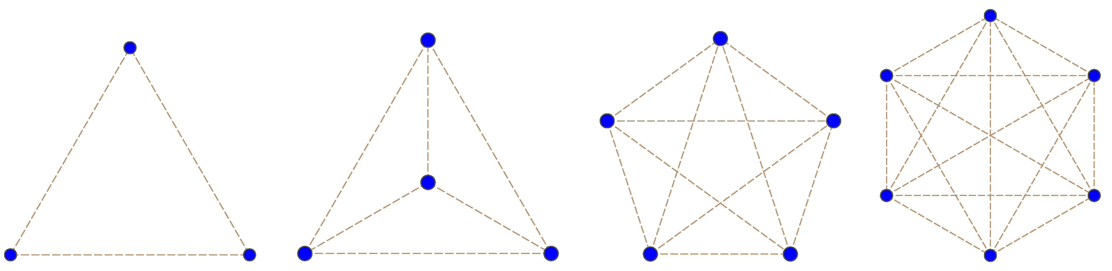
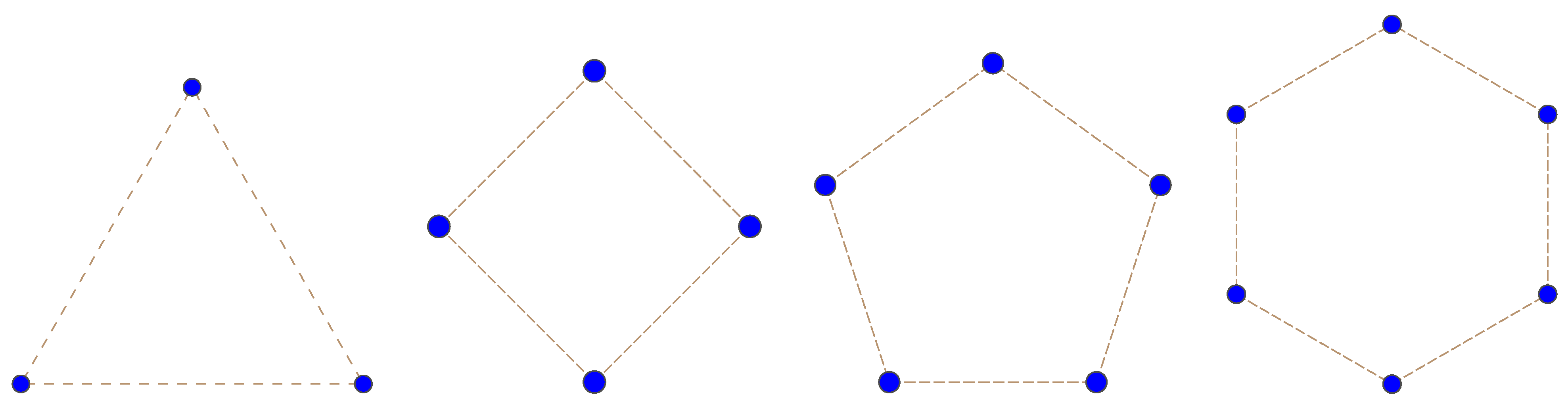
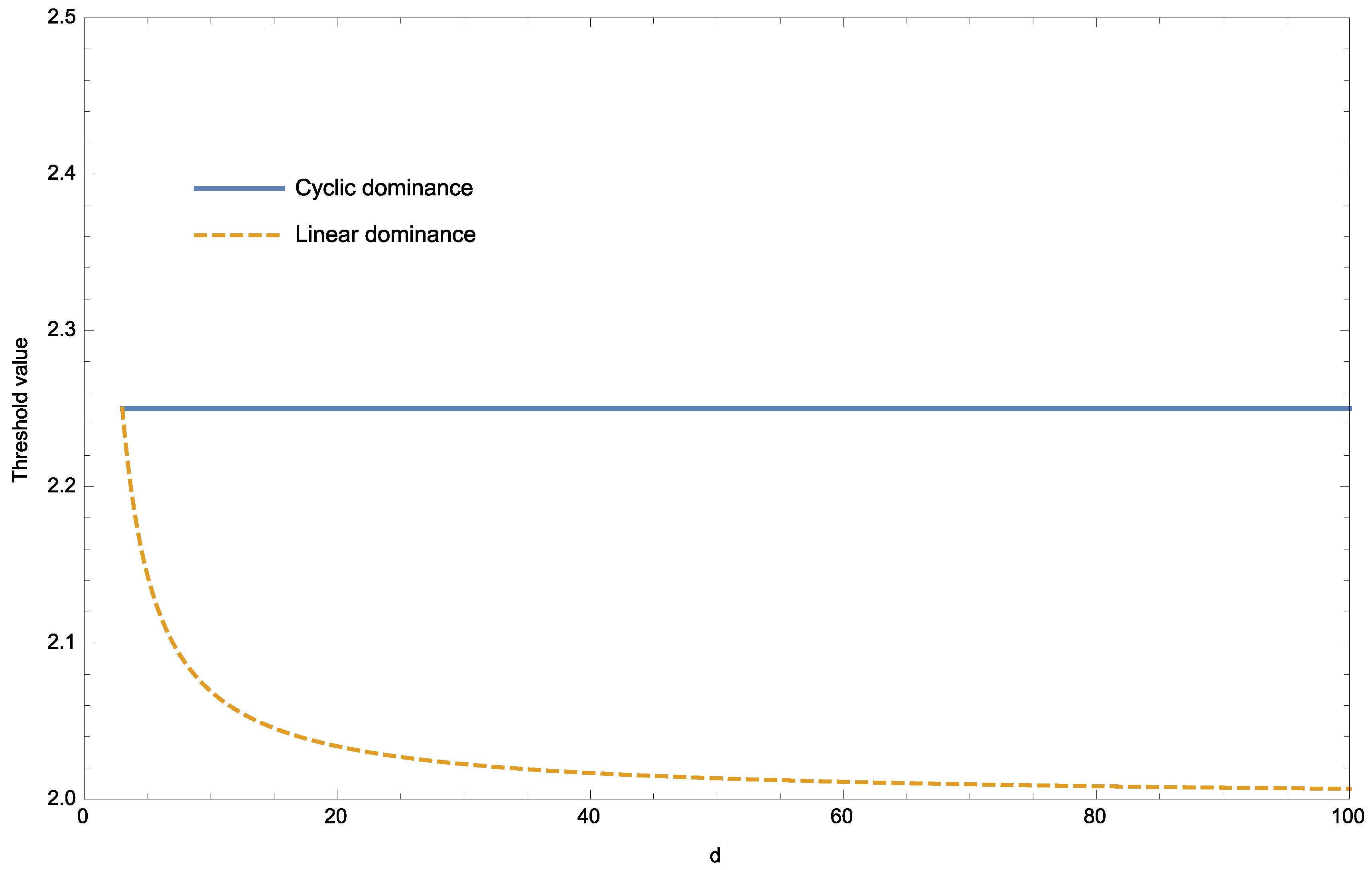
Our main result has been applied to the situation of dominance hierarchy with d colonies in decreasing order of dominance in the case of linear dominance and in counter-clockwise order of dominance in the case of cyclic dominance. Individuals in a given colony can interact with individuals in all other colonies in the case of linear dominance, but only with individuals in the same colony or in the two adjacent colonies in the case of cyclic dominance. Considering the strategies TFT and AllD in a repeated additive prisoner’s dilemma and a cost for defection against a dominant defector, it has been shown that linear dominance is more favourable than cyclic dominance for increasing the expected frequency of TFT at equilibrium as soon as $d>3$. This has been obtained under the assumptions of colonies of the same size with uniform or symmetric migration and random interactions.

Another application concerns the set-structured population as introduced in Tarnita et al. [26], but with colonies of fixed relative sizes and reproduction according to a Moran model instead of a Wright–Fisher model. With uniform mutation from one subset of sets to another of the same size, which defines the phenotype of an individual, the condition for $S_1$ to be favoured by weak selection is that, for an individual chosen at random in the whole population, the expected payoff of $S_1$ exceeds the expected payoff of $S_2$ near neutrality. With strategy $S_1$ actually used only if the number of common sets to which the two players belong exceeds some threshold, it has been shown that the condition for $S_1$ to be favoured by weak selection reduces to a condition known as risk dominance (Harsanyi and Selten [39]) as in a well-mixed population. Note that the same result was obtained in Tarnita et al. [26] in the case of a high rate of phenotype mutation, which corresponds to strong migration from one phenotype to another.

9. Conclusions

Conditions for a strategy to be more abundant on average at equilibrium than another strategy in a structured population under weak selection and weak strategy mutation but strong migration can be expressed in terms of reproductive values in the neutral model on the basis of a two-time scale argument. This can be applied, for instance, to two-player games in populations with set structure or dominance hierarchy. In the case of dominance hierarchy, it has been shown that the condition for $TFT$ to be more abundant on average than $AllD$ in a repeated additive prisoner’s dilemma with a given cost for defection against a dominant defector is generally less stringent with linear dominance than with cyclic dominance. In the case of set structure with strong migration from one set to another, it has been shown that the condition for a strategy to be more abundant on average than another corresponds to risk dominance.

References

1. Nagylaki, T. The strong-migration limit in geographically structured populations. J. Math. Biol. 1980, 9, 101–114. [Google Scholar] [CrossRef] [PubMed]
2. Notohara, M. The strong-migration limit for the genealogical process in geographically structured populations. J. Math. Biol. 1993, 31, 115–122. [Google Scholar] [CrossRef]
3. Herbots, H.M. The structured coalescent. In Progress in Population Genetics and Human Evolution; Donnelly, P., Tavare, S., Eds.; Springer: New York, NY, USA, 1997; pp. 231–255. [Google Scholar]
4. Kingman, J.F.C. On the genealogy of large populations. J. Appl. Probab. 1982, 19, 27–43. [Google Scholar] [CrossRef]
5. Kingman, J.F.C. Exchangeability and the evolution of large populations. In Exchangeability in Probability and Statistics; Koch, G., Spizzichino, F., Eds.; North-Holland Publishing Company: Amsterdam, The Netherlands, 1982; pp. 97–112. [Google Scholar]
6. Kingman, J.F.C. The coalescent. Stoch. Process. Their Appl. 1982, 13, 235–248. [Google Scholar] [CrossRef]
7. Axelrod, R.M.; Hamilton, W.D. The evolution of cooperation. Science 1981, 211, 1390–1396. [Google Scholar] [CrossRef] [PubMed]
8. Szabò, G.; Tóke, C. Evolutionary prisoner’s dilemma on a square lattice. Phys. Rev. E 1998, 58, 68. [Google Scholar] [CrossRef]
9. Traulsen, A.; Röhl, T.; Schuster, H.G. Stochastic gain in population dynamics. Phys. Rev. Lett. 2004, 93, 028701. [Google Scholar] [CrossRef] [PubMed]
10. Santos, F.C.; Pacheco, J.M. Scale-free networks provide a unifying framework for the emergence of cooperation. Phys. Rev. Lett. 2005, 95, 098104. [Google Scholar] [CrossRef] [PubMed]
11. Hauert, C.; Szabò, G. Game theory and physics. Am. J. Phys. 2005, 73, 405–414. [Google Scholar] [CrossRef]
12. Nowak, M.A. Five rules for the evolution of cooperation. Science 2006, 314, 1560–1563. [Google Scholar] [CrossRef] [PubMed]
13. Nowak, M.A. Super Cooperators; Free Press: New York, NY, USA, 2011. [Google Scholar]
14. Nowak, M.A.; Sigmund, K. How populations cohere: Five rules for cooperation. In Theoretical Ecology, 3rd ed.; May, R., McLean, A., Eds.; Oxford Press: Oxford, UK, 2007. [Google Scholar]
15. Ohtsuki, H.; Nowak, M.A.; Pacheco, J.M. Breaking the symmetry between interaction and replacement in evolutionary dynamics on graphs. Phys. Rev. Lett. 2007, 98, 108106. [Google Scholar] [CrossRef] [PubMed]
16. Szabò, G.; Fáth, G. Evolutionary games on graphs. Phys. Rep. 2012, 446, 97–216. [Google Scholar] [CrossRef]
17. Hamilton, W.D. The genetic of social behaviour I. J. Theor. Biol. 1964, 7, 1–16. [Google Scholar] [CrossRef]
18. Hamilton, W.D. The genetic of social behaviour II. J. Theor. Biol. 1964, 7, 17–32. [Google Scholar] [CrossRef]
19. Trivers, R.L. The evolution of reciprocal altruism. Q. Rev. Biol. 1971, 46, 35–37. [Google Scholar] [CrossRef]
20. Frank, S.A. Foundations of Social Evolution; Princeton University Press: Princeton, NJ, USA, 1998. [Google Scholar]
21. Nowak, M.A.; Sigmund, K. Evolution of indirect reciprocity by image scoring. Nature 1998, 393, 573–577. [Google Scholar] [CrossRef] [PubMed]
22. Nowak, M.A.; Sigmund, K. The dynamics of indirect reciprocity. J. Theor. Biol. 1998, 194, 561–571. [Google Scholar] [CrossRef] [PubMed]
23. Nowak, M.A. Evolutionary Dynamics; The Belknap Press of Harvard University Press: Cambridge, MA, USA, 2006. [Google Scholar]
24. Traulsen, A.; Nowak, M.A. Evolution of cooperation by multi-level selection. Proc. Natl. Acad. Sci. USA 2006, 103, 10952–10955. [Google Scholar] [CrossRef] [PubMed]
25. Kroumi, D.; Lessard, S. Evolution of cooperation in a multidimensional phenotype space. Theor. Popul. Biol. 2015, 102, 60–75. [Google Scholar] [CrossRef] [PubMed]
26. Tarnita, C.E.; Antal, T.; Ohtsuki, H.; Nowak, M.A. Evolutionary dynamics in set structured populations. Proc. Natl. Acad. Sci. USA 2009, 106, 8601–8604. [Google Scholar] [CrossRef] [PubMed]
27. Hammerstein, P. The role of asymmetries in animal contests. Anim. Behav. 1981, 29, 578–581. [Google Scholar] [CrossRef]
28. Wilson, E.O. Sociobiology: The New Synthesis; Belknap Press: Cambridge, MA, USA, 1975. [Google Scholar]
29. Tao, Y.; Xu, J.J.; Li, C.; Cressman, R. Dominance hierarchies induce a population’s full cooperation. Dyn. Games Appl. 2014, 4, 432–447. [Google Scholar] [CrossRef]
30. Kroumi, D.; Lessard, S. Conditions for cooperation to be more abundant than defection in a hierarchically structured population. Dyn. Games Appl. 2014, 5, 239–262. [Google Scholar] [CrossRef]
31. Möhle, M. A convergence theorem for Markov chains arising in population genetics and the coalescent with selfing. Adv. Appl. Probab. 1973, 30, 493–512. [Google Scholar] [CrossRef]
32. Nowak, M.A.; Tarnita, C.E.; Antal, T. Evolutionary dynamics in structured populations. Philos. Trans. R. Soc. B 2010, 365, 19–30. [Google Scholar] [CrossRef] [PubMed]
33. Moran, P.A.P. Random processes in genetics. Proc. Camb. Philos. Soc. 1958, 54, 60–71. [Google Scholar] [CrossRef]
34. Moran, P.A.P. Statistical Processes of Evolutionary Theory; Clarendon Press: Oxford, UK, 1962. [Google Scholar]
35. Krebs, J.R.; Davies, N.B. An Introduction to Behaviour Ecology; Blackwell Publishing: Oxford, UK, 1982. [Google Scholar]
36. Walters, J.R.; Seyfarth, R.M. Conflict and cooperation. In Primate Societies; Smuts, B.B., Cheney, D.L., Seyfarth, R.M., Wrangham, R.W., Struhsaker, T., Eds.; University of Chicago Press: Chicago, IL, USA, 1982; pp. 306–317. [Google Scholar]
37. Axelrod, R.M. The Evolution of Cooperation; Basic Books: New York, NY, USA, 1984. [Google Scholar]
38. Linhart, S. Some thoughts on the Ken game in Japan: From the viewpoint of comparative civilization studies. Senri Ethnol. Stud. 1995, 40, 101–124. [Google Scholar]
39. Harsanyi, J.C.; Selten, R. A General Theory of Equilibrium Selection in Games; MIT Press: Cambridge, MA, USA, 1988. [Google Scholar]
40. Lessard, S. Effective game matrix and inclusive payoff in group-structured populations. Dyn. Games Appl. 2011, 2, 301–318. [Google Scholar] [CrossRef]
41. Culver, W.J. On the existence and uniqueness of the real logarithm of a matrix. Proc. Am. Math. Soc. 1973, 17, 1146–1151. [Google Scholar] [CrossRef]
42. Higham, N.J. Functions of Matrices: Theory and Computation; Society for Industrial and Applied Mathematics (SIAM): Philadelphia, PA, USA, 2008. [Google Scholar]