
The Evolvability of Cooperation under Local and Non-Local Mutations

Department of Biology, University of Pennsylvania, Philadelphia, PA 19104, USA
*
Author to whom correspondence should be addressed.
Games 2015, 6(3), 231-250; https://doi.org/10.3390/g6030231
Submission received: 23 May 2015
/
Revised: 17 July 2015
/
Accepted: 17 July 2015
/
Published: 23 July 2015
(This article belongs to the Special Issue Cooperation, Trust, and Reciprocity)
Abstract
:We study evolutionary dynamics in a population of individuals engaged in pairwise social interactions, encoded as iterated games. We consider evolution within the space of memory-1strategies, and we characterize all evolutionary robust outcomes, as well as their tendency to evolve under the evolutionary dynamics of the system. When mutations are restricted to be local, as opposed to non-local, then a wider range of evolutionary robust outcomes tend to emerge, but mutual cooperation is more difficult to evolve. When we further allow heritable mutations to the player’s investment level in each cooperative interaction, then co-evolution leads to changes in the payoff structure of the game itself and to specific pairings of robust games and strategies in the population. We discuss the implications of these results in the context of the genetic architectures that encode how an individual expresses its strategy or investment.
1. Introduction
Cooperation is a puzzle. Although it is intuitively obvious that pairs or groups of individuals can benefit from mutual cooperation, pinning down precisely when and how and for how long cooperation will occur is surprisingly difficult. This is especially true in evolution [1,2,3,4,5,6,7]. In an evolving population, individuals change their behavior through random mutations and reproduce according to fitness; thus, strategies evolve through trial and error alone. In an evolving system, the question of whether cooperation will arise depends not only on whether stable cooperative strategies exist, but also on whether natural selection can find such strategies. It depends on the evolvability of cooperation.
Evolvability is the capacity of a system to generate adaptive mutations [8,9]. This depends critically on the genetic architecture underlying the evolving trait [10,11,12]. It depends on what kind of mutations are produced and at what frequency. In this paper, we investigate the evolvability of cooperation under repeated pairwise social interactions, modeled as an iterated two-player game with memory-1 strategies (Figure 1). We show that, when strategy mutations are local as opposed to non-local: (i) a wider variety of evolutionary outcomes tends to occur (ii); mutual cooperation is much harder to evolve; and (iii) mutual cooperation persists for much longer if it does evolve. We also show that when the investment in cooperative behavior is allowed to evolve alongside the strategy for when to cooperate, a still wider variety of evolutionary outcomes is possible, with different pairings of investments and strategies arising in the same system.
Figure 1.
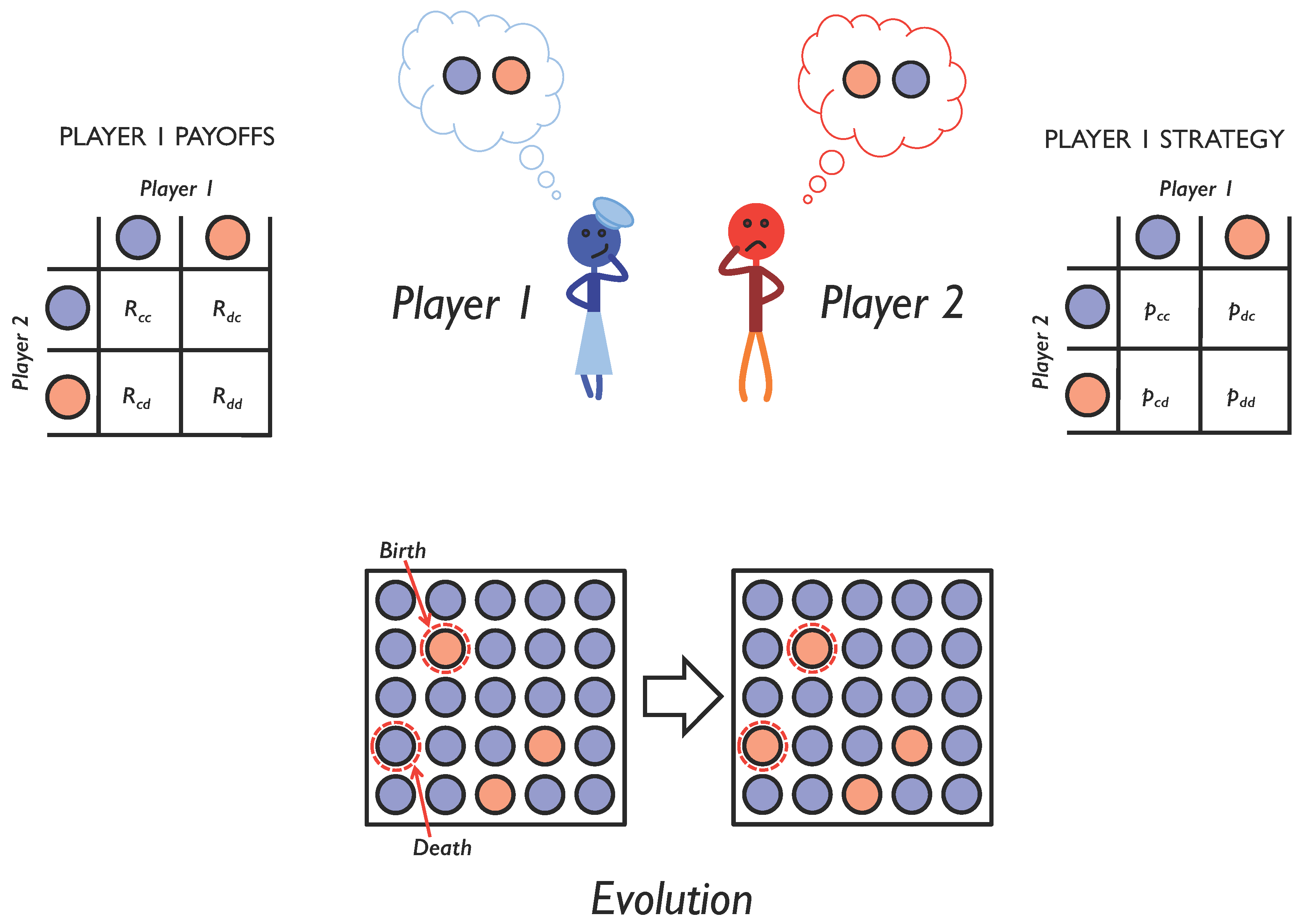
Evolving social interactions. We study repeated pairwise social interactions using iterated games. Over the course of multiple interactions, players choose whether to cooperate (blue circle) or defect (red circle), depending on the outcome of their previous interaction. A player’s probability of cooperation given her previous interaction is encoded as a memory-1 strategy (right). Depending on the outcome of each interaction, she receives a payoff (left). To study the evolution of social interactions, we assume that each player’s reproductive success is proportional to the payoff she receives from all social interactions with all other members of the population. This leads to an evolution in the strategies used in the population (bottom) and allows us to explore the conditions under which cooperation will emerge.
Figure 1.
Evolving social interactions. We study repeated pairwise social interactions using iterated games. Over the course of multiple interactions, players choose whether to cooperate (blue circle) or defect (red circle), depending on the outcome of their previous interaction. A player’s probability of cooperation given her previous interaction is encoded as a memory-1 strategy (right). Depending on the outcome of each interaction, she receives a payoff (left). To study the evolution of social interactions, we assume that each player’s reproductive success is proportional to the payoff she receives from all social interactions with all other members of the population. This leads to an evolution in the strategies used in the population (bottom) and allows us to explore the conditions under which cooperation will emerge.
These results illustrate that the evolvability of cooperation depends critically on both the type of mutations underlying the evolution of social behavior and the size of their effects. Different model choices lead to qualitatively different expectations for when and how cooperation will evolve, the types of strategies and even the types of games we might expect to find in nature. Thus, understanding the genetic architecture that encodes the range of strategies and investment schemes allowable to an organism by genetic mutations is a prerequisite for predicting the patterns of behavior that will arise in an evolving population.
2. Results
2.1. Iterated Two-Player Games
We study the evolution of cooperation in a finite population of N individuals. In each generation, each member of the population engages in pairwise social interactions with every other member of the population. The social interaction consists of an infinitely iterated two-player game. In each round of the game, both players simultaneously choose whether to cooperate or defect (Figure 1). In each round the players receive payoffs depending on their play and their opponent’s play, where the subscripts indicate the outcome of the round, and the focal player’s play is listed first. We assume and , so that mutual cooperation is always more beneficial than mutual defection and unilateral cooperation always less beneficial than unilateral defection. Note that these assumptions allow for games in which mutual cooperation is always most beneficial () or in which mutual defection is always the worst outcome (). We assume that each player’s reproductive success is proportional to her average payoff across all games played against all members of the population.
In this study, we focus on the effects of local mutations, which alter a player’s strategy or investment by a small amount, on evolutionary dynamics. We assume that each local mutation is introduced into a monomorphic population, as is typical when studying adaptive dynamics. We look for strategies that form stable fixed points of these evolutionary dynamics. In general, a strategy that is a fixed point must have a selection gradient equal to zero, except for the special case when a fixed-point strategy lies on the boundary of strategy space. For an interior fixed point, stability is determined by the curvature of the fitness landscape around the fixed point. In this study, we start by showing that, with a particular exception that has been classified elsewhere, interior fixed points with a zero-selection gradient never occur in the space of memory-1 strategies for two-player iterated games. Thus, we need not perform any analysis of the curvature of the fitness landscape around such fixed points in our study. Instead, our analysis is focused on the selection gradient at the boundaries, where the only fixed points in our system can occur. Stable strategies at the boundary of the strategy space, which have a non-zero selection gradient facing perpendicular to the boundary, are necessarily neighbored by other strategies of the same character. Mutations that move strategies parallel to the boundary are neutral, and as a result, there exist regions of stable strategies, all of which are evolutionary robust, rather than strict evolutionary stable strategies.
We consider populations in which each player i is characterized by a memory-1 strategy, , which determines her probability of cooperation in the current round of the iterated game, given the outcome of the preceding round (where once again, the subscripts indicate the outcome of the preceding round and the focal player’s play is listed first). We will first consider evolution occurring in the four-dimensional space of memory-1 strategies. In order to do this, it is convenient to use an alternate coordinate system [13,14,15,16] defined by:
This coordinate system allows us to obtain the following identity for the payoff of player i and a similar one for the payoff of player j:
where denotes the equilibrium payoff to player i with the strategy played against player j with the strategy . We write for the equilibrium rates of the different plays in a given iterated game. For notational convenience in what follows, we also write as the equilibrium rate of opposite play between the two players (i.e., the outcome or ). By definition, the rate of opposite play is symmetrical between the two players, i.e., . Note that the parameterization of the coordinate transform used here is slightly different from that used in [15,16], in order to simplify the analysis of dynamics under local mutations. Furthermore, note that the space of viable strategies is the unit four-cube, and extremal strategies in the alternate coordinate system are obtained by setting the probabilities for cooperation to either one or zero in Equation (1). The equilibrium payoff to player i can be found by solving a pair of simultaneous equations (of the form Equation (2)), for the two player’s scores to give:
Furthermore, when from Equation (2), we see that both players receive the payoff:
As in previous studies of iterated games [15,16,17], we will assume that there is a small amount of noise ϵ in the execution of a strategy, such that the play at equilibrium does not depend on the first move (i.e., the Markov chain associated with the iterated game has a unique equilibrium distribution without absorbing states) [18]. We will now use Equations (1)–(4) to determine the stable points of the evolutionary dynamics under local mutations, using the framework of adaptive dynamics.
2.2. Adaptive Dynamics of Memory-1 Strategies
In the framework of adaptive dynamics, a homogenous population is assumed monomorphic at all times and assumed to evolve towards the mutants with the highest invasion fitness [19,20,21]. This framework is used to describe the evolution of well-mixed populations under local mutations. The stable states of such a system can be determined by looking at the selection gradient. In what follows we are looking for the conditions that be an equilibrium, i.e. the point with . Since we assume an individual’s fitness is proportional to her average payoff, we recover selection gradient:
where we have used:
to account for the effect that an invader faces opponents of the resident strategy in a population of size N [21,22]. Because a strategy p consists of probabilities, which must lie in the range , Equation (5) permits two kinds of stable equilibria: (i) a strategy with zero selection gradient (corresponding to a fixed point of the evolutionary dynamics) and negative curvature around the fixed point (corresponding to a Jacobian whose eigenvalues have negative real components); and (ii) a strategy at the boundary of strategy space with the selection gradient perpendicular to and facing towards the boundary. We refer to strategies that are stable equilibria of the evolutionary dynamics under local mutations as locally-evolutionary robust, in contrast to strategies that are robust against all possible, non-local mutants under strong selection, which we call globally-evolutionary robust. The latter notion, global robustness, is discussed in detail in [16]. Note that the globally-evolutionary robust strategies are necessarily a subset of the locally-evolutionary robust strategies.
2.2.1. Zero Selection Gradient
A zero selection gradient, which ensures a fixed point of the adaptive dynamics, can only be produced in the following ways (see Materials and Methods):
- and
- and
- and
The first case requires a population of size and is not of particular evolutionary interest.
The second case corresponds to an equalizer strategy [23], which ensures . These strategies are discussed in [14,16,20,23] and are unstable fixed points under both local and non-local mutations.
The third case contains a number of possible sub-cases. However, we find (see Materials and Methods) that there are no viable strategies that produce a zero selection gradient, except at the boundaries of strategy space. Thus, the only locally-robust strategies under local mutations lie at the boundary of strategy space. The same result also holds under non-local mutations [16]. Because the stable equilibria of this system all lie at the boundaries of strategy space and involve non-zero selection gradients, we do not in general need to determine the stability of the system by looking at the eigenvalues around a fixed point, as would be typical for a dynamical system of this type. Instead, it is sufficient to look at whether the selection gradient at the boundary is directed towards or away from it.
2.2.2. Selection Gradient Perpendicular into the Boundary
A strategy with the selection gradient perpendicular to and pointing towards the boundary of strategy space can only be produced in the following ways (see Materials and Methods):
- and ;
- and ;
- and simultaneously take extremal values.
The first case corresponds to a zero-determinant (ZD) strategy with or . The adaptive dynamics of ZD strategies are discussed in detail in [20]. We only add here that those strategies that are locally-robust within the space of ZD strategies are also locally robust within the full space of memory-1 strategies.
The second case corresponds to or . These are the self-cooperators [13,15,16,24] and self-defectors as defined in [16]. The set of locally-robust self-cooperators and self-defectors, and , is given by:
The third case contains four sub-cases (see Materials and Methods). The first sub-case corresponds to and . These are the self-alternators described in [16]. These strategies have and . The set of locally-robust self-alternators, , is given by:
The second sub-case corresponds to and , so that and . Such a strategy is always unstable (see Materials and Methods). The third sub-case corresponds to and , which have and . These strategies alternate between mutual cooperation and mutual defection, and they are unstable (see Materials and Methods). The final sub-case corresponds to and , which implies . These strategies are always unstable (see Materials and Methods).
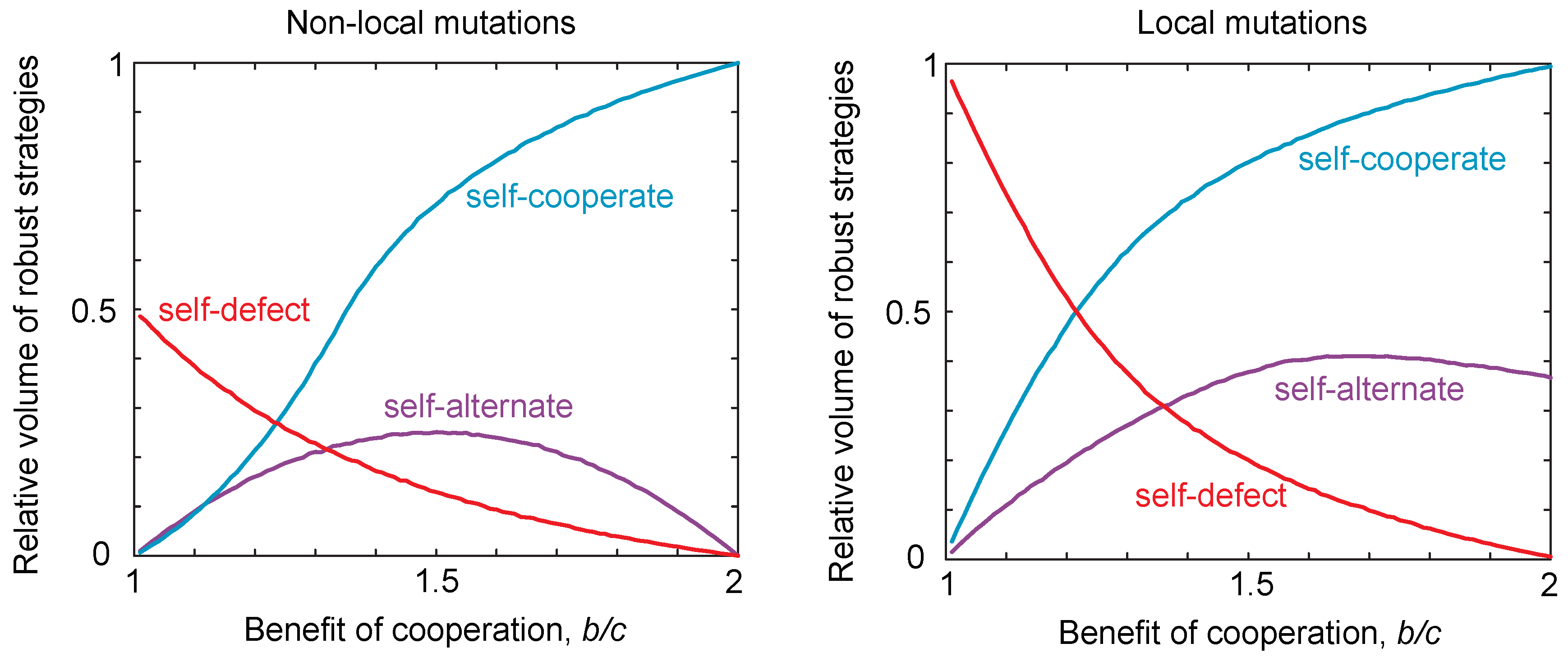
Thus, there are only three possible classes of locally-robust strategies: self-cooperators, self-defectors and self-alternators. These three classes of strategies are summarized and compared to the case of non-local mutations in Figure 2. We discuss those strategies that lie at the intersection of multiple classes in the Materials and Methods. The volumes of locally-robust self-cooperators, self-defectors and self-alternators are defined as the probability that a randomly-drawn strategy of each class satisfies Equations (7) or (8). Robustness is thus defined relative to the total volume of the strategy class, which allows us to compare the robust volumes of each class despite the fact that the self-alternators are two-dimensional whilst the self-cooperators and self-defectors are three-dimensional. We can then compare the volume of robust strategies in the case of local mutations to the volume of strategies that are robust to non-local mutations as described in [16]. This is shown in Figure 2. We see that the patterns are qualitatively the same for local and non-local mutations, as we vary the benefits for cooperation. However, we see that the volume of self-defecting strategies in particular tends to be greater under local mutations compared to global mutations. That is, local mutations tend to increase the propensity for defecting strategies to be evolutionary robust.
2.3. Probability of Reaching a Strategy Class
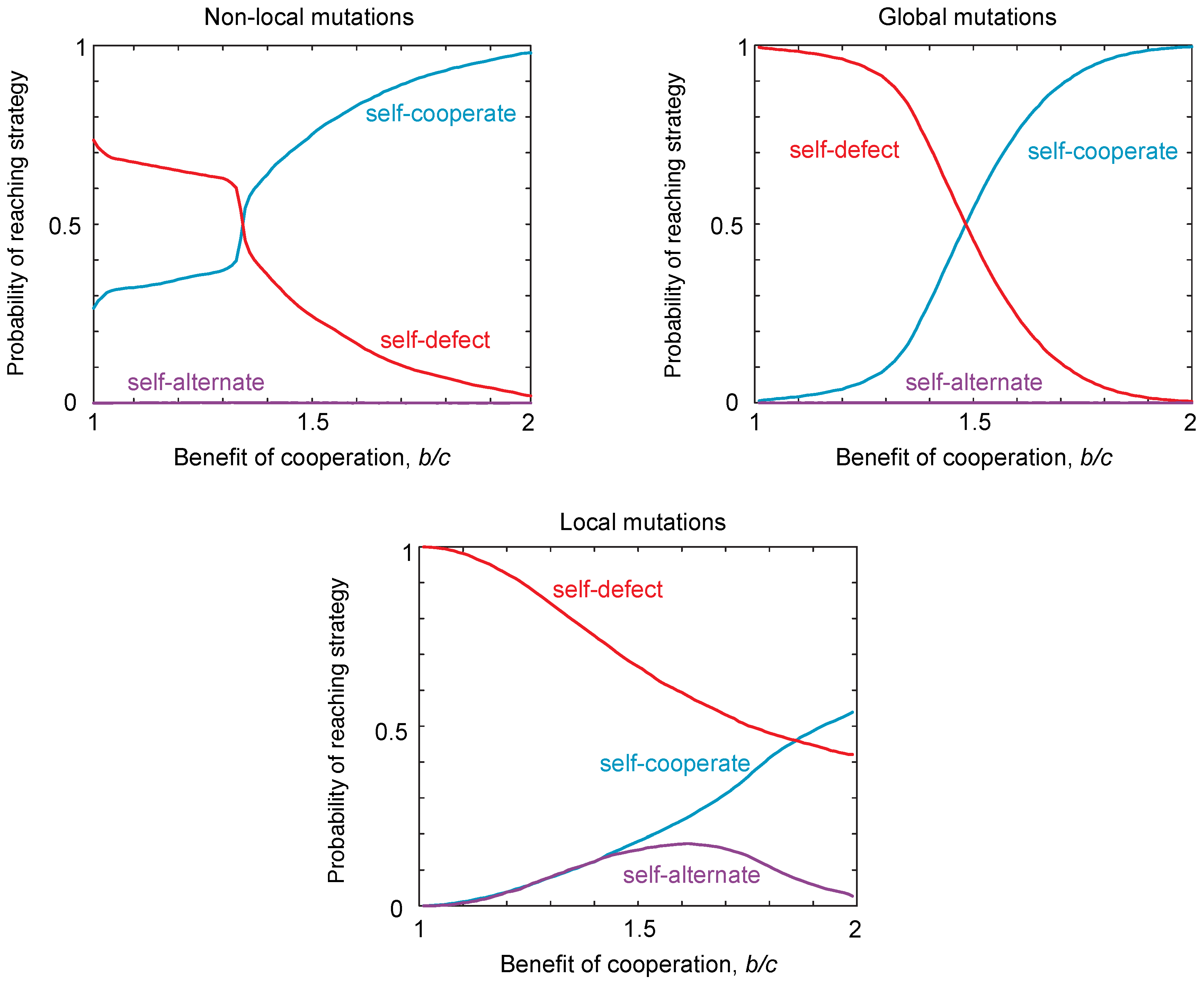
We have identified three classes of strategy that can be locally robust, which correspond to the same qualitative classes of globally-robust strategies identified previously [16]. However, to investigate the evolvability of cooperation, we must also consider the probability of reaching the different classes of robust strategies from the interior of the strategy space. The probability of reaching a strategy class depends on the starting strategy at which the population is initialized. We calculate the probability of reaching each strategy class from a randomly-chosen starting strategy. In Figure 3, we use Monte Carlo simulations to quantify the probability of reaching each of the three robust classes of strategies. We contrast these probabilities of reaching each class in the case of local mutations to the case of non-local mutations (Figure 3). These simulations reveal that, under local mutations, the robust self-defecting class is relatively easier to reach than in the case of non-local mutations, whereas robust self-cooperators are relatively harder to reach. Thus, from the point of view of evolvability, local mutations make self-cooperating strategies more difficult to evolve, in the sense that fewer evolutionary trajectories from random starting conditions lead to robust outcomes.
Figure 2.
Robust volumes under local and non-local mutations. We considered populations playing an iterated public goods game, with payoffs , , and . For non-local mutations, we numerically integrated to determine the robust volumes of the different strategy classes, based on the conditions for robustness given in [16], namely for self-cooperate, for self-defect and for self-alternate. For local mutations, we used the local stability conditions given in Equations (7) and (8). We varied the ratio of costs to benefits and calculated the volume for each resulting payoff. We see the same qualitative trend in both cases; however, the volume of robust self-defecting strategies is greater in the non-local compared to the local case.

Quite surprisingly, local mutations make self-alternate much easier to evolve for some choices of payoff, and the probability of reaching these strategies varies non-monotonically with the benefits for cooperation (Figure 3a). Thus, local mutations can substantially alter the types of strategies that readily evolve compared to the case of non-local mutations. This result is particularly striking, because the probability of reaching a strategy class is comparable for both the three-dimensional set of self-cooperators and self-defectors, as well as for the two-dimensional set of self-alternators.
Figure 3.
The probability of reaching different strategy classes under local, non-local and global mutations. We simulated populations playing an iterated public goods game, with payoffs , , and . To determine the probability of reaching each strategy class, we drew initial conditions and simulated evolution until the population was within of a robust strategy class. Simulations were carried out under weak mutation according to the “copying” process [35], such that a population is initially monomorphic with resident strategy i, until a new mutant strategy j arises and fixes in the population, with probability , where s is the selection strength, set to , so that evolution is under strong selection when mutations are non-local, and is the payoff of strategy i against strategy j, calculated according to Equation (3). For non-local mutations, one of the four probabilities for cooperation, was redrawn with uniform probability in the range , with the other three probabilities left unchanged. For global mutations, all four probabilities for cooperation were redrawn with uniform probability in the range . For local mutations, one of the four probabilities for cooperation was increased or decreased by δ with equal probability. We numerically determined the probability of reaching each robust strategy type, for different ratios of costs to benefits . The results show significant differences in the probability of reaching different strategy classes between local and non-local mutations. In particular, the probability of reaching self-defect is larger and of reaching self-cooperate smaller, under local mutations. In addition, self-alternate has a significant probability of being reached for intermediate values of under local mutations, but not for non-local or global mutations.
2.4. Neutral Drift
The probability of reaching a strategy class is not the whole story. Once a population arrives at a locally-robust strategy, which sits on the boundary of strategy space and has a selection gradient perpendicular to the boundary, mutations occurring parallel to the boundary are neutral. For example, for a robust self-cooperator strategy with , mutations to , or have no effect on fitness. Once a population arrives at a robust self-cooperator strategy, such neutral mutations will subsequently fix with probability in a finite population, and so, unconstrained variables undergo drift over time. However, if the unconstrained variables drift to values that do not satisfy the robustness condition Equation (7), the direction of selection on will flip, and the population will transiently move away from the self-cooperators.
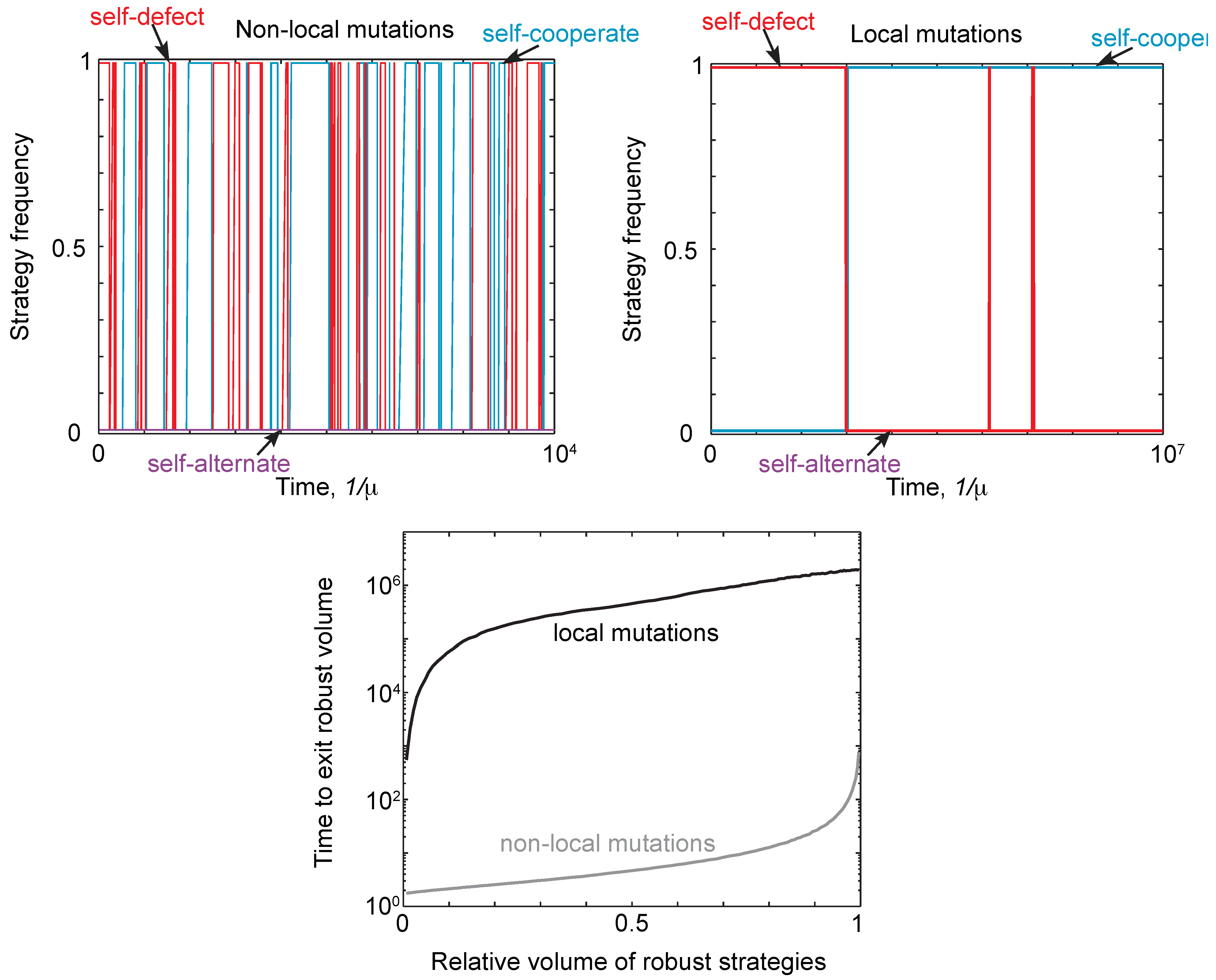
Thus, neutral drift can allow a population to eventually move away from a robust strategy type. This phenomenon is illustrated in Figure 4 for local and non-local mutations. Starting at a robust self-defector, strategies drift until the self-defectors are eventually replaced by robust self-cooperators (or robust self-alternators), and vice versa. In other words, starting at a robust strategytype, the population will always eventually leave that type. The timescale for this turnover of strategies is far shorter under non-local mutants than under local mutations. This is further illustrated in Figure 4, which shows the mean time to drift to a non-robust strategy under local and non-local mutations, as a function of the volume of robust strategies at which the population starts.
In summary, our results on the probability of reaching a strategy class and the dynamics of neutral drift show that mutual cooperation is harder to evolve, but persists for longer once it arises, under local versus non-local mutations.
2.5. Evolution of Investment
So far, we have offered little discussion of payoffs, besides constraining and . However, as shown in [16], under non-local mutation, allowing the investment in cooperation to evolve alongside the strategy determining whether to cooperate can radically alter evolutionary outcomes.
We now consider the co-evolution of payoffs and strategies under local mutations. We assume each player i has an investment level , such that she pays cost each time she cooperates and receives benefit due to the investment of both her and her opponent. We assume that a player i who defects in a given round invests . We can thus consider the five-dimensional system in which players are characterized by strategy p and investment level x. The resulting payoffs for a player i are then:
Figure 4.
Neutral drift under local and non-local mutations. (Top) We simulated evolution under weak mutation, as described in Figure 3, initializing populations with the strategy always as defect, , and payoffs and . We compared the trajectories for a single run under local and non-local mutations, comparing the frequency of self-cooperate, self-defect and self-alternate strategies. The population was assigned to a particular strategy class if it was within distance of that class. For non-local mutations, there is a rapid turnover of different strategy types, despite the population spending most of its time at self-cooperate or defect. For local mutations, the rate of turnover is many orders of magnitude slower, with mutations only producing one turnover event between self-defect and self-cooperate. (Bottom) We calculated the time, averaged over starting conditions, for a population to drift out of a region of robust strategies as a function of the volume. As expected, it takes far longer for the population to drift away from a region of robust strategies under local mutations, resulting in the slower turnover of strategy types seen in the top right panel.

Because the equilibrium plays do not depend on the payoffs of the game, the selection gradient for the strategies taken at and is once again given by Equation (5). In addition, the selection gradient for the investment level is given by:
and recall that is the equilibrium rate of the play , etc. As before, there are four possible stable equilibrial solutions to Equation (5), corresponding to the locally-robust strategies of Equations (7) and (8): self-cooperators for which and ; self-defectors for which and ; and self-alternators for which and . Equations (5) and (10) together therefore have three possible stable equilibria. For self-defectors, the level of investment evolves neutrally (i.e., all values of x are stable). Whereas for self-cooperators, the stable equilibrium satisfies:
and for self-alternators, the stable equilibrium satisfies:
Depending on the function , Equations (12) and (13) may have solutions that correspond to qualitatively different games (i.e., payoff matrices with different rank orderings of entries).
To illustrates this phenomenon, we consider a sigmoid benefit function:
where h determines the slope of the function and determines the threshold value, such that when , . This choice of benefit function makes intuitive sense, because it increases monotonically with the level of investment, but saturates when investments become very large. Given a benefit function of this form, Equations (12) and (13) each have a single stable equilibrium (see the Materials and Methods) given by an investment level of:
for self-cooperate and:
for self-alternate.
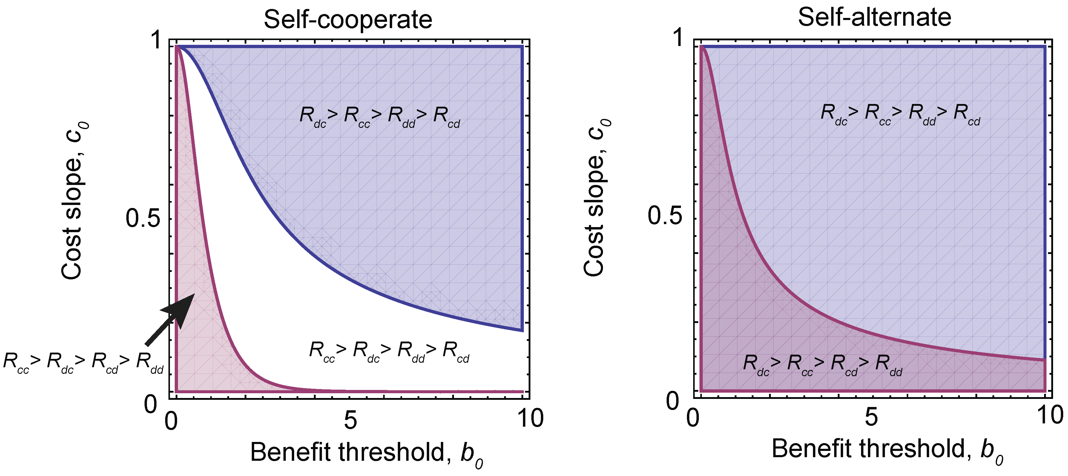
We can use these results to determine which pairs of games and strategies are robust against local mutations. These are shown in Figure 5. We find that there are stable solutions that consist of self-cooperate, paired with three different payoff orderings, depending on the choice of parameters , and h. Conditioning on , which is required for a stable equilibrium solution (see the Materials and Methods), we find that self-cooperate can be paired with a prisoner’s dilemma, a stag hunt or a harmony game, while self-alternate can be paired with a prisoner’s dilemma or a snowdrift game. In other words, these are the only robust pairings of strategy types and game types that can arise under evolution with local mutations. However, it is important to note that for a given (fixed) set of payoffs, there are in general multiple robust strategies types.
Figure 5.
The evolution of different games. Under a sigmoidal benefit function (Equation (13)), different pairs of strategies and investment levels are robust (Equations (14) and (15)). Depending on the choice of threshold in the benefit function, , and the slope of the rate of change of the cost of cooperation with investment, (where we have fixed the slope of the sigmoid ), this can result in different orderings of payoffs and, hence, different equilibrium games. (Left) The equilibrium games paired with self-cooperating strategies. The blue region has payoff ordering and corresponds to a prisoner’s dilemma. However, in the white region , which corresponds to a stag hunt game, and in the red region , a harmony game. (Right) When self-alternate dominates, only two games are possible. The blue region is again a prisoner’s dilemma, while the purple region has and is a snowdrift game.
3. Discussion and Conclusions
The problem of understanding the evolution of cooperation has two components. The first is to understand whether cooperation can be evolutionary stable [22,25,26]. This depends on the costs and benefits of cooperation [5,16,27,28], on the population structure [27,28] and on the environment [29,30,31]. As we have shown here, it also depends, to some extent, on the types of mutations that can occur, whether they are local or non-local, and which aspects of cooperative behavior are able to evolve. The second component to understanding the evolution of cooperation is to determine whether natural selection can produce those cooperative behaviors that are evolutionary stable. That is, it depends on whether cooperation is evolvable. We have shown here that both the tendency of evolution to find stable cooperative behaviors and how long those behaviors can persist in the presence of neutral drift differ substantially depending on whether mutations are local or non-local.
An important conclusion from our results is that local mutations can substantially alter the types of robust strategies that are likely to evolve. In particular, local as opposed to non-local mutations can substantially increase the chance for self-alternating strategies to evolve (Figure 3). When strategies and investment levels co-evolve, this in turn can alter the types of games that evolve under local vs. non-local mutations and may in general lead to an increase in snowdrift game-like payoff structures, as opposed to prisoner’s dilemma or stag hunt payoff structures (Figure 4). Of central importance to our analysis of the evolutionary dynamics in memory-1 strategy space is the role of neutral drift in determining how long different strategy types will persist. Neutral drift may alter the evolutionary dynamics still further if we relax the assumption of weak mutation; that is if mutations occur at a substantial rate and significant variation is maintained in the population. In such a scenario, the length of time the population remains at a particular strategy class may be significantly altered, as a mixture of stable and unstable strategies of the same type may quickly arise in the population. Furthermore, the type of drift among strategies of the same class we describe may not be strictly neutral in a natural population if, for example, there are costs associated with maintaining a strategic response to punishing defectors. Mutations that reduce costs by eliminating the ability to punish defectors may in fact be selectively favored when cooperation dominates. In such a scenario, self-cooperate may tend to be lost more rapidly in favor of self-defect than in the strictly neutral case shown in Figure 4.
Our results all highlight the need to understand the genetic architecture that underlies social behaviors if we are to understand behavioral evolution. While this goal may be a long way off when it comes to human behavior, it is likely more accessible when studying the evolution of cooperation in simple micro-organisms [4]. As we have seen in this study and elsewhere [32,33], if an organism is able to react to a previous interaction and evolve both the response and the investment level in cooperation, then a fairly wide array of both strategic behaviors and types of game can evolve spontaneously. Furthermore, factors such as spatial structure and evolutionary branching [34] can lead to an even richer set of evolutionary outcomes, all of which make this a fascinating area for future study.
4. Materials and Methods
Here, we determine the equilibrium solutions to Equations (5) and (11) for the adaptive dynamics of memory-1 strategies and the levels of investment in cooperation.
4.1. Evolution of Memory-1 Strategies under Local Mutations
An equilibrium solution can occur in two ways in this system. When the selection gradient is zero, the resident strategy of the population is a fixed point of the adaptive dynamics. The stability of the fixed point (stable, unstable or saddle point) can be determined by looking at the Jacobian and through simulation.
Because viable strategies must lie in the range , it is also possible for an equilibrium solution of the adaptive dynamics to lie at the boundary of strategy space, such that the selection gradient on the variable taking an extremal value is directed towards the boundary, and the selection gradient on the other variables (which, in general, do not take an an extremal value) is zero. In this case, the selection gradient is perpendicular to the boundary. Any strategy that satisfies these conditions must be a stable fixed point of the evolutionary dynamics.
We will first consider the case in which the four variables do not take extremal values and look for fixed points with a selection gradient of zero. The coordinate transform from the strategy p to the alternate coordinate system is given in Equation (1). The inverse transform is given by:
From Equation (16), we can immediately deduce the following:
We can calculate the equilibrium rate of opposite play explicitly [14] from:
It will also be necessary to calculate the selection gradient in the original p coordinate system, since local stability can vary under a non-linear coordinate transformation. This is related to the selection gradient of the by:
and we see immediately that the selection gradient Equation (19) is zero if the selection gradient Equation (5) is zero.
4.1.1. Selection Gradient away from the Boundaries
As noted above, in order for Equation (5) to be zero, we must have either , or . The first case is not of interest in an evolving population, for which . The second case, , defines a ZD strategy [14], whose evolutionary dynamics are discussed in [20]. From Equation (17), the third case can only be satisfied if . Combining this with Equation (19) and solving the resulting set of simultaneous equations using Mathematica, we find that this can occur either when , when or when . The first two cases lie on the boundary of strategy space and are dealt with below. The third case also requires . This system of equations can be solved explicitly using Mathematica to yield solutions . However, solving for p to give zero selection gradient in Equation (5) shows that the only solution is , i.e., always defect. Thus, there are no stable solutions to the evolutionary dynamics except at the boundaries.
4.1.2. Selection Gradient at the Boundaries
At the boundaries, since implies , we must either have zero selection gradient on both ϕ and χ, or else, both must take an extremal value and have selection gradient towards the boundary. We first look at the extremal values of κ.
Extremal values of κ: These occur when or . As mentioned above, this gives . It also gives a rate of equilibrium play , and the selection gradient on the other three parameters is zero. In order for a given solution to be stable, the selection gradient on κ must be positive for self-cooperate and negative for self-defect. This gives the classes of locally-robust strategies, Equation (7).
Extremal values of ϕ and χ: Looking next at the extremal values of ϕ and χ, we see from Equation (1) that the sum is maximized when and . For these strategies, Equation (18) reveals , and Equation (17) shows that the direction of selection must be positive on both χ and on ϕ for the strategy to be a stable equilibrium. In addition, the equilibrium rate of play for this strategy gives , and , so that the selection gradient on is zero. Finally, this strategy gives , its maximum value, so that the selection gradient on must be positive for stability. Converting to the original p coordinate system using Equation (19), we see that this implies that the selection gradient on must be negative and the gradient on positive, while the other gradients are zero. This gives the condition Equation (8) for the local stability of the self-alternators.
Similarly to the previous case, the sum is minimized when and . This again gives a maximum value of ; however from Equation (19) (and as shown in [16]), selection always acts to decrease , and so, these strategies are unstable.
The difference is maximized when and . Similarly to the self-alternators, this gives where the selection on χ must be negative and on ϕ positive for stability. The selection gradient on is zero. We also find from Equations (17) and (18) that for this strategy. However, calculating using Equations (17) and (18), we find that selection is always to increase and decrease , and the strategy is always unstable (as is also shown in [16]).
Finally, the difference is minimized when and . However, selection on these strategies always favors an increase in , and they are unstable [16]. Note that this strategy corresponds to a minimal value of , and we have thus implicitly dealt with both extremal values of .
4.1.3. Intersection of Multiple Strategy Classes
Strategies may lie in more than one of the class of locally-robust strategies described above. In particular, the strategy tit-for-tat lies at the intersection of all three strategy classes. However, as discussed in [16], strategies belonging to multiple classes are typically unstable and will tend to evolve towards a single class that maximizes the mutual payoff of interacting players.
4.2. Evolution of Investment
The solutions to Equations (11) and (12) for a sigmoidal benefit function as given by Equation (13) are and , respectively. Each has two solutions for x:
and:
where is required for the solutions to be real. Looking at the second derivatives, we find that the solution is a stable equilibrium iff , which, in turn, implies , which gives the single solution Equations (14) and (15).
Acknowledgments
We thank Charles Mullon and Todd Parsons for helpful discussions. J.B.P. acknowledges funding from the Burroughs Wellcome Fund, the David and Lucile Packard Foundation, US Department of the Interior Grant D12AP00025, and Foundational Questions in Evolutionary Biology Fund Grant RFP-12-16.
Author Contributions
Alexander J. Stewart and Joshua B. Plotkin designed and conducted the research and wrote the manuscript.
Conflicts of Interest
The authors declare no conflict of interest.
References
- Axelrod, R.; Axelrod, D.E.; Pienta, K.J. Evolution of cooperation among tumor cells. Proc. Natl. Acad. Sci. USA 2006, 103, 13474–13479. [Google Scholar] [CrossRef] [PubMed]
- Axelrod, R. The Evolution of Cooperation; Basic Books: New York, NY, USA, 1984. [Google Scholar]
- Boyd, R.; Gintis, H.; Bowles, S. Coordinated punishment of defectors sustains cooperation and can proliferate when rare. Science 2010, 328, 617–620. [Google Scholar] [CrossRef] [PubMed]
- Cordero, O.X.; Ventouras, L.A.; DeLong, E.F.; Polz, M.F. Public good dynamics drive evolution of iron acquisition strategies in natural bacterioplankton populations. Proc. Natl. Acad. Sci. USA 2012, 109, 20059–20064. [Google Scholar] [CrossRef] [PubMed]
- Nowak, M.A. Five rules for the evolution of cooperation. Science 2006, 314, 1560–1563. [Google Scholar] [CrossRef] [PubMed]
- Van Dyken, J.D.; Wade, M.J. Detecting the molecular signature of social conflict: Theory and a test with bacterial quorum sensing genes. Am. Nat. 2012, 179, 436–450. [Google Scholar] [CrossRef] [PubMed]
- Waite, A.J.; Shou, W. Adaptation to a new environment allows cooperators to purge cheaters stochastically. Proc. Natl. Acad. Sci. USA 2012, 109, 19079–19086. [Google Scholar] [CrossRef] [PubMed]
- Draghi, J.; Wagner, G.P. The evolutionary dynamics of evolvability in a gene network model. J. Evolut. Biol. 2009, 22, 599–611. [Google Scholar] [CrossRef] [PubMed]
- Masel, J.; Trotter, M. Robustness and evolvability. Trends Genet. 2010, 26, 406–414. [Google Scholar] [CrossRef] [PubMed]
- Draghi, J.; Wagner, G.P. Evolution of evolvability in a developmental model. Evolution 2008, 62, 301–315. [Google Scholar] [CrossRef] [PubMed]
- Draghi, J.; Parsons, T.; Wagner, G.; Plotkin, J. Mutational robustness can facilitate adaptation. Nature 2010, 436, 353–355. [Google Scholar] [CrossRef] [PubMed]
- Stewart, A.; Parsons, T.; Plotkin, J. Environmental robustness and the adaptability of populations. Evolution 2012, 66, 1598–1612. [Google Scholar] [CrossRef] [PubMed]
- Akin, E. Stable Cooperative Solutions for the Iterated Prisoner’s Dilemma. 2012. arXiv:1211.0969. Available online: http://arxiv.org/abs/1211.0969v1 (accessed on 21 July 2015).
- Press, W.H.; Dyson, F.J. Iterated Prisoner’s Dilemma contains strategies that dominate any evolutionary opponent. Proc. Natl. Acad. Sci. USA 2012, 109, 10409–10413. [Google Scholar] [CrossRef] [PubMed]
- Stewart, A.J.; Plotkin, J.B. From extortion to generosity, evolution in the Iterated Prisoner’s Dilemma. Proc. Natl. Acad. Sci. USA 2013, 110, 15348–15353. [Google Scholar] [CrossRef] [PubMed]
- Stewart, A.J.; Plotkin, J.B. Collapse of cooperation in evolving games. Proc. Natl. Acad. Sci. USA 2014, 111, 17558–17563. [Google Scholar] [CrossRef] [PubMed]
- Hilbe, C.; Nowak, M.A.; Sigmund, K. Evolution of extortion in Iterated Prisoner’s Dilemma games. Proc. Natl. Acad. Sci. USA 2013, 110, 6913–6918. [Google Scholar] [CrossRef] [PubMed]
- Fudenberg, D.; Maskin, E. Evolution and Cooperation in noisy repeated games. Am. Econ. Rev. 1990, 80, 274–279. [Google Scholar]
- Geritz, S.; Kisdi, E.; Meszéna, G.; Metz, J. Evolutionarily singular strategies and the adaptive growth and branching of the evolutionary tree. Evolut. Ecol. Res. 1998, 12, 35–37. [Google Scholar] [CrossRef]
- Hilbe, C.; Nowak, M.A.; Traulsen, A. Adaptive dynamics of extortion and compliance. PLoS ONE 2013, 8, e77886. [Google Scholar] [CrossRef] [PubMed]
- Imhof, L.A.; Nowak, M.A. Stochastic evolutionary dynamics of direct reciprocity. Proc. Biol. Sci. 2010, 277, 463–468. [Google Scholar] [CrossRef] [PubMed]
- Hilbe, C. Local replicator dynamics: A simple link between deterministic and stochastic models of evolutionary game theory. Bull. Math. Biol. 2011, 73, 2068–2087. [Google Scholar] [CrossRef] [PubMed]
- Boerlijst, M.C.; Nowak, M.A.; Sigmund, K. Equal pay for all prisoners. Am. Math. Month. 1997, 104, 303–307. [Google Scholar] [CrossRef]
- Stewart, A.J.; Plotkin, J.B. Extortion and cooperation in the Prisoner’s Dilemma. Proc. Natl. Acad. Sci. USA 2012, 109, 10134–10135. [Google Scholar] [CrossRef] [PubMed]
- Hofbauer, J.; Sigmund, K. Evolutionary Games and Population Dynamics; Cambridge University Press: Cambridge, UK, 1998. [Google Scholar]
- Page, K.M.; Nowak, M.A. Unifying evolutionary dynamics. J. Theor. Biol. 2002, 219, 93–98. [Google Scholar] [CrossRef]
- Lieberman, E.; Hauert, C.; Nowak, M.A. Evolutionary dynamics on graphs. Nature 2005, 433, 312–316. [Google Scholar] [CrossRef] [PubMed]
- Ohtsuki, H.; Hauert, C.; Lieberman, E.; Nowak, M.A. A simple rule for the evolution of cooperation on graphs and social networks. Nature 2006, 441, 502–505. [Google Scholar] [CrossRef] [PubMed]
- Cabrales, A. Stochastic replicator dynamics. Int. Econ. Rev. 2000, 41, 451–482. [Google Scholar] [CrossRef]
- Foster, D.; Young, P. Stochastic evolutionary game dynamics. Theor. Popul. Biol. 1990, 38, 219–232. [Google Scholar] [CrossRef]
- Fudenberg, D.; Harris, C. Evolutionary dynamics with aggregate shocks. J. Econ. Theory 1992, 57, 420–441. [Google Scholar] [CrossRef]
- Wang, Z.; Szolnoki, A.; Perc, M. Different perceptions of social dilemmas: Evolutionary multigames in structured populations. Phys. Rev. E 2014, 90, 032813. [Google Scholar] [CrossRef]
- Perc, M.; Szolnoki, A. Coevolutionary games—A mini review. Biosystems 2010, 99, 109–125. [Google Scholar] [CrossRef] [PubMed]
- Doebeli, M.; Hauert, C.; Killingback, T. The evolutionary origin of cooperators and defectors. Science 2004, 306, 859–862. [Google Scholar] [CrossRef] [PubMed]
- Traulsen, A.; Nowak, M.A.; Pacheco, J.M. Stochastic dynamics of invasion and fixation. Phys. Rev. E 2006, 74, 011909. [Google Scholar] [CrossRef]
© 2015 by the authors; licensee MDPI, Basel, Switzerland. This article is an open access article distributed under the terms and conditions of the Creative Commons Attribution license (http://creativecommons.org/licenses/by/4.0/).
Share and Cite
MDPI and ACS Style
Stewart, A.J.; Plotkin, J.B. The Evolvability of Cooperation under Local and Non-Local Mutations. Games 2015, 6, 231-250. https://doi.org/10.3390/g6030231
AMA Style
Stewart AJ, Plotkin JB. The Evolvability of Cooperation under Local and Non-Local Mutations. Games. 2015; 6(3):231-250. https://doi.org/10.3390/g6030231
Chicago/Turabian StyleStewart, Alexander J., and Joshua B. Plotkin. 2015. "The Evolvability of Cooperation under Local and Non-Local Mutations" Games 6, no. 3: 231-250. https://doi.org/10.3390/g6030231