Article

Inefficient Learning Leads to Efficient Coordination: A Repeated Stag-Hunt Game with Learning Agents


1
IMT School for Advanced Studies, 55100 Lucca, Italy
2
Institute of Cognitive Sciences and Technologies (ISTC), National Research Council, 00196 Rome, Italy
3
Grupo Interdisciplinar de Sistemas Complejos (GISC), Departamento de Matemáticas, Universidad Carlos III de Madrid, 28911 Leganés, Spain
4
Centro Studi Dinamiche Complesse (CSDC), University of Florence, 50019 Sesto Fiorentino, Italy
5
Deptartment of Physics and Astronomy, University of Florence, 50019 Sesto Fiorentino, Italy
6
Department of Education, Literatures, Intercultural Studies, Languages and Psychology, University of Florence, 50129 Florence, Italy
*
Author to whom correspondence should be addressed.
Games 2026, 17(4), 39; https://doi.org/10.3390/g17040039
Submission received: 18 June 2026 / Revised: 16 July 2026 / Accepted: 21 July 2026 / Published: 23 July 2026
(This article belongs to the Section Learning and Evolution in Games)

Abstract

In coordination games, the distinctive presence of multiple equilibria poses a challenge to coordination, and this has led over time to the proposal of numerous determinants of the latter. In this paper, we study coordination in a repeated Stag-hunt game played by two agents who are able to learn from the outcomes of each game, but do not know the payoff matrix. By modulating their learning capabilities, we show that agents are able to coordinate on the social optimum when they learn slowly from experience and are prone to making mistakes. A comparison with the results from a recent laboratory experiment is also provided.

1. Introduction

The emergence of cooperation among humans has become a significant area of research since the late XX Century (Axelrod, 1981; Challet & Zhang, 1997). Much of this body of work examines the evolutionary dynamics that favor altruistic behavior in natural environments, framing the issue as a problem of population dynamics (Hofbauer & Sigmund, 1998; Roca et al., 2009b). However, cooperation is pervasive and can also be observed in pair interactions within competitive contexts. In this type of interaction, cooperation between both individuals is usually desirable, as it allows everyone to obtain the maximum possible benefit, the so-called social optimum. But from an individual point of view, the choice to cooperate is not always so straightforward. In some scenarios, cooperating or defecting may be the best and safest choice for the individual, regardless of the actions of the other, making it easier to make a decision (or predict actions). However, in other situations, this is not always the case: there is no universal best choice, and predicting the implications of one’s decisions becomes more difficult, as they are conditioned by the actions of the other.
In game theory, this situation of strategic uncertainty is formally described by the existence of multiple Nash equilibria, outlining a fundamental coordination problem. To study this phenomenon, numerous frameworks, under the name of coordination games, have been proposed. In these settings, unlike social dilemmas characterized by an implicit conflict of interest, players achieve better results if they make the same choices, with the consequent absence of a unique dominant strategy (Devetag & Ortmann, 2014).
From a theoretical point of view, the presence of multiple equilibria represents a deadlock: standard equilibrium analysis does not allow behavioral predictions to be made, forcing theorists to be agnostic about the actual equilibrium selection. As highlighted by Cooper and Weber (2020), this gap has stimulated experimental exploration of coordination, revealing a general tendency for people to coordinate, albeit not always on the most efficient outcome (Cooper & Weber, 2020; Devetag & Ortmann, 2014). In this broad and diverse strand of literature, scholars have investigated different aspects and possible determinants of coordination. Sociocultural factors (e.g., Chen & Chen, 2011; De Kwaadsteniet & Van Dijk, 2010; Engelmann & Normann, 2010; Fallucchi & Nosenzo, 2022; Krupka et al., 2022; Krupka & Weber, 2013), such as the existence of shared social representations and cultural standards, may facilitate successful coordination thanks to their effect on players’ expectations (implicit or otherwise). Studies on cognitive aspects, on the other hand, have instead investigated internal reasoning processes, exploring decision-making styles (intuitive vs. deliberative) and players’ levels of sophistication (e.g., Arad & Rubinstein, 2012; Bardsley et al., 2010; Belloc et al., 2019; Camerer et al., 2004; Nagel, 1995; Rubinstein, 2016; Stahl & Wilson, 1995). The question of equilibrium selection has also been extensively addressed by more theoretical strands of the literature, such as evolutionary game theory. These numerical studies have investigated coordination games in both well-mixed populations and network structures, testing different update rules, such as myopic best response or imitative mechanisms (Raducha & San Miguel, 2022). These studies have shown how topological features can, in some cases, facilitate coordination (Tomassini & Pestelacci, 2010; Vilone et al., 2021), although this kind of effect is not generally universal (Roca et al., 2009a). Finally, a minority of studies have explored coordination by moving away from the evolutionary approach in favor of cognitive and learning mechanisms (Flache & Macy, 2002; Macy & Flache, 2002; Roth & Erev, 1995; Skyrms, 2004). A common feature of these works is the use of relatively simple learning processes and a deliberately unsophisticated representation of the agents’ cognitive mechanisms. By eschewing the traditional assumption of perfect rationality, this perspective reveals that coordination on the social optimum can be successfully achieved even through minimal adaptive heuristics.
Following this latter perspective, in this work, we studied the coordination dynamics between two agents who participate in a repeated coordination game. In particular, we explored how fundamental learning processes can shape cooperation and strategic coordination in an exclusively pair-wise interaction, where the dynamics of the game and the strategic outcomes are initially unknown and more than one Nash equilibrium is possible. The objective of this work is twofold, as it aims to (i) model some recent experimental results and (ii) to show how simple and imperfect cognitive mechanisms are sufficient to navigate strategic uncertainty and resolve coordination problems in dyadic settings, without the need to employ complex deductive reasoning.
The paper is organized as follows: Section 2 provides the general configuration and dynamics of the model; the results obtained from the numerical simulations and a comparison with some recent experimental results are reported in Section 3. Finally, Section 4 discusses the results, limitations, and future prospects.

2. Materials and Methods

A classic game-theory framework that investigates coordination between two agents is the Stag-hunt (SH) game (Skyrms, 2001). The game represents a situation in which two hunters can cooperate to capture a larger prey, the Stag, or decide not to do so and settle for a smaller one (Hare). In the first case, the payoff is greater, but there is a risk of getting nothing if the other player decides not to cooperate. In the other case, the hare does not require coordination between the two players and represents a guaranteed payoff, albeit smaller than that of the Stag. This scenario inevitably generates tension between two strategic criteria, payoff and risk dominance, resulting in two possible equilibria. In the first case, both agents coordinate by choosing Stag. This is the Pareto-optimal and payoff-dominant equilibrium, as both players will obtain the maximum expected payoff. On the other hand, agents both choose Hare, obtaining a secure but significantly lower payoff. This risk-dominant equilibrium is the result of the strategic uncertainty inherent in the SH game: choosing Hare is in fact an optimal strategy given the high risk of miscoordination. The SH game therefore exhibits two pure Nash equilibria, and once one of these is reached, the agents have no incentive to change their strategy.
The following paragraphs in this section describe the general configuration adopted for the SH game, the update rule that governs the strategic choices of agents, and the different scenarios tested.

2.1. General Configuration

Let us consider two players,“player 1” and “player 2,” engaged in a repeated SH game. Each agent i is characterized by a probability p i S of choosing Stag (S), while p i H = 1 p i S is the complementary probability of choosing Hare (H). Depending on their chosen strategy, each player receives a reward determined by the payoff matrix P ^ given in Table 1, before updating the probability of the adopted strategy according to the overall reward obtained up to that round of the game.
When both agents choose Stag, the payoff obtained by each player is given by r + ε , where r is the gain for (Hare, Hare) and the parameter ε represents the coordination prize for both moving on Stag. It is important to note that in this version of the game, a player adopting the Hare strategy gains the reward r independently of the opponent’s choice. The introduction of this variation allowed us to test the ability of the players to learn the best option even though the alternative guaranties the same reward in any case. This makes such SH closer to a Prisoner’s Dilemma game, with the difference being that the best option here is also a Nash equilibrium. At the end of each round, the agents’ cumulative payoff (that is, the sum of all the rewards received up to that round) is updated based on the strategies adopted.
Finally, it is important to emphasize that in the experiments we refer to in this work, players can check the other agent’s behavior, while in this theoretical framework, they choose their strategy without knowing the opponent’s decision (see Section 3.3 and Appendix A). It is noteworthy that, despite this strong simplification, the results of our simulations are nevertheless in good agreement with the empirical findings, as we are going to see in the following sections.

2.2. Dynamics

2.2.1. Initial Conditions

Regarding the initial strategies, at the time step t = 0 , the probability that each agent will choose Stag, p i S , is equal to p 1 S = p 2 S = 0.5 = p 1 H = p 2 H . This implies that, at the beginning of each simulation, agents do not know the rules of the game and the payoffs associated with the strategies.
As regards the cumulative payoff, in the experimental setup of this game (see again Section 3.3 and Appendix A), players lose a small amount of their payoff at each round, because it is assumed that just playing costs some energy, and if one player reaches zero energy, the game ends. Therefore, in order to be as coherent as possible with the experiments, we assign each agent an initial endowment of 10 units of payoff at the beginning of each realization. Every time they play a game stage, they lose 0.5 units, with this quantity representing the effort players put into playing the game, and if one of the agents continues to have no energy (that is, zero payoff), the simulation stops. Regardless, in all the simulations performed in every scenario tested, the agents managed to never reach zero (which happened in the experiments shown in Section 3.3 and Appendix A), so we are no longer going to mention it in the following sections.

2.2.2. Update Rule

At the end of each round of the game, players update the probabilities associated with the two strategies based on the payoff obtained. More precisely, if the player i has chosen the strategy K at the N-th stage, the probability of choosing K will be updated according to the following learning rule:
p i K ( n e w ) = p i K + α i ( 1 p i K ) Π K i ( r + ε ) N ,
where α i is the learning rate of the player i, Π K i is the total amount of reward gained by the player until the N-th stage when adopting the strategy K, and the normalization factor 1 / [ ( r + ε ) N ] guarantees that p i K [ 0 , 1 ] at each time. Of course, since p i S + p i H 1 , the probability to adopt the other strategy will change accordingly as well.
The learning rate α i ( 0 , 1 ] of each agent i is assigned during initialization and does not vary over time. This parameter modulates the impact of the result obtained by the strategy K adopted at the time step t, dictating the extent to which the agent reacts to the experiences. Specifically, at the beginning of each single run of the model, agents 1 and 2 are assigned α 1 and α 2 , respectively, whose values remain constant for the entire duration of the simulation and are chosen from the interval ( 0 , 1 ] . Through this initial assignment, we can test different scenarios in which agents exhibit the same, similar, or different learning rates, enabling us to study how coordination evolves in pairs of agents with homogeneous or heterogeneous learning capabilities. Overall, the introduction of this parameter allows us to increase the realism of the model, representing the cognitive abilities of the agent, as well as allowing us to study the interaction of heterogeneous agents, characterized by different values of α .

2.2.3. Error Probability

At the beginning of each round, each agent i adopts a strategy K based on the corresponding probability p i K . This implies that a successful strategy, in terms of payoff, will have a higher probability of being adopted. This mechanism, although not deterministic, does not take into account the possibility that the agent makes mistakes. For this reason, among some of the scenarios, we will include an error probability μ i , assigned to each agent and constant over time. In these cases, agent i initially determines the strategy K to adopt based on p i K ; once the strategy has been selected, agent i can choose the opposite strategy with probability μ i .

2.3. Simulations

The learning rates α i and the error probabilities μ i allowed us to explore different scenarios. The first case (baseline model) that we tested refers to the representation of perfectly rational agents, where players exhibit the highest learning rate ( α 1 = α 2 = 1 ) and do not make mistakes ( μ 1 = μ 2 = 0 ). Next, we evaluated the impact of the learning rate alone by testing different combinations of the values of α 1 and α 2 (keeping μ 1 = μ 2 = 0 ). Similarly, we repeated the simulations to evaluate the influence of the probabilities of error μ alone on agents’ strategies, for different combinations of μ 1 and μ 2 , while keeping α 1 = α 2 = 1 . Finally, we investigated the combined effect of both learning rate and error probability.
For each scenario, we studied the impact of r [ 1 , 10 ] on the evolution of the probabilities associated with the two strategies: Stag and Hare. After assigning the agents their respective values for the parameters α and μ , we performed T = 10 3 independent simulations for each scenario and value of r and computed the final average probabilities. For each run, agents continued to interact until convergence or the maximum number of iterations ( t = 10 5 ) was reached. The convergence criterion was satisfied if the change in the probability of each agent, p 1 S and p 2 S , was less than ϵ < 0.01 over a time window of 10 2 consecutive iterations.

3. Results

3.1. Baseline Model

In the baseline version of the model, we set α i = 1 and μ i = 0 , i . Therefore, agents learn at the fastest pace possible and never make mistakes. Considering perfectly rational learning agents is of course a huge approximation, we nevertheless start with this toy version for two main reasons: firstly, if we are able to capture some of the experimental results with such simplified model, this would indicate that the selected features are sufficiently powerful to provide a reasonable description of reality; secondly, it can work as a baseline to compare the effect of further refinements of the model itself.
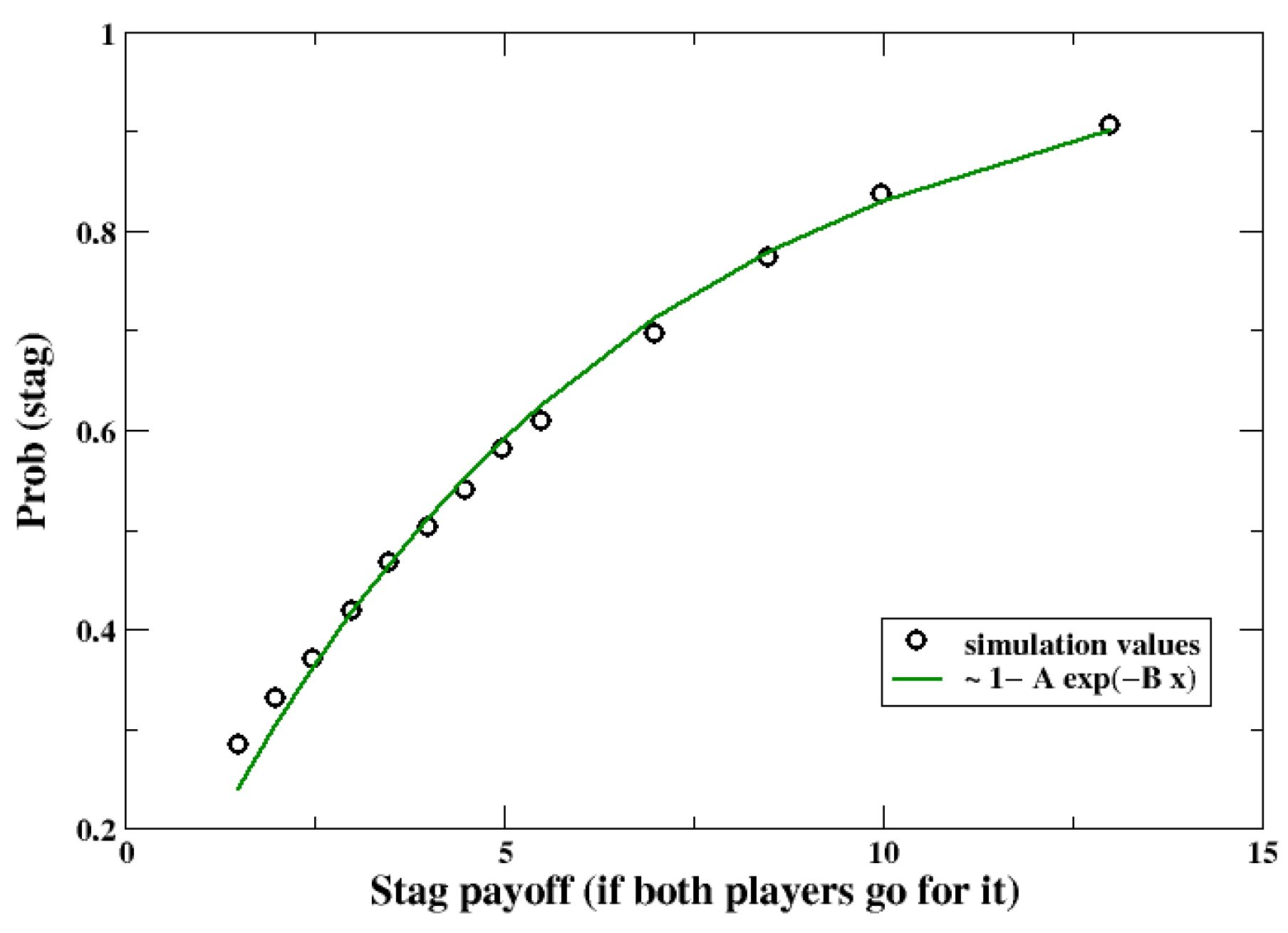
Figure 1 reports the average probability of the two agents choosing Stag (S), which is equivalent to the probability that a single simulated experiment ends up with players always choosing S. As is easy to see, for r + we have p S 1 : an expected outcome, since if the Stag option is infinitely more profitable than Hare, there is no chance that the Hare choice can be selected.
When r = 4 , the average probability that both agents choose S is p S = 0.5 . This indicates that players learn with a probability larger than 50 % that ( S , S ) is actually the best option when the associated reward is at least four times more profitable than the Hare’s payoff.
This outcome can theoretically be justified as follows. From Equation (1), we can write down the average elementary variation Δ P t of the probability p S after the t th interaction (of course, the same can be done for p H = 1 p S ). Assuming that α i = 1 , i , and that, by symmetry, the probability of choosing the strategy K evolves equally for both players, we obtain the following after a few passages:
Δ P t S = P t S ( 1 P t S ) P t S Π S Π H ( r + ε ) t ,
where
Π s = j = 0 N ( P j S ) 2 · ( r + ε ) ; Π h = j = 0 N ( 1 P j S ) · r ,
that are the average rewards gained up to the N-th round when a player has adopted the Stag/Hare strategy, respectively. From Equation (2), it is easy to see that P N S = P * = 0 and P N S = P + = 1 are two fixed points of the dynamics, which is confirmed in simulations since, for every independent run, both players end up with the probability of choosing Stag equal to 0 or 1 for both, i.e., they always coordinate. There is also a third equilibrium, P ¯ , that is,
P ¯ = Π H Π S .
Now, if P ¯ is a physical equilibrium, that is, if P ¯ ( 0 , 1 ) , then it is unstable. Indeed, let us assume that both players have reached P S = P ¯ . If they go again to Stag, for the rule given in Equation (1), at the subsequent stage, the probability will tend to increase again and go away from P ¯ .
Therefore, we have established in a single run that players coordinate, with the final configuration always being one where both players always go for the Stag or always go for the Hare. We can evaluate the probability that a single run ends up with both players choosing the Stag, i.e., we can explain the results shown in Figure 1. To this end, let us consider the interactions in the very early stages of the game, when we can pose p S = p H = 0.5 for both players. Focusing on a given player, its probability to choose Stag at the first interaction will change as follows:
Δ p 0 S = 1 2 with probability 1 4 r 2 ( r + ε ) with probability 3 4
Of course, on average, the double Stag is always the best configuration for the interacting players, but since they do not know the rewards at the beginning, they have to discover that it is the most convenient option just by trying. Now, in order to understand that mutual Stag is the best option, both players have to go for both on S to collect the payoff: on average, this happens once every four runs. More precisely, in the early stages of the game, both players select the strategy at random so that with a probability of 1 / 4 only, they go for the Stag at the same time: therefore, for r 4 only, it becomes convenient for the Stag strategy, as it rightly appears in the figure.

3.2. Learning Rate and Error Probability

In the baseline model, agents update the probability of choosing Stag based on the payoffs obtained. The impact of the latter is maximal and, in the first interactions, it is able to significantly modify the behavior of agents. Furthermore, decisions are not subject to errors and agents possess the same characteristics. However, this scenario may not represent reality. Humans do not learn at the same speed and are prone to making mistakes. In order to better capture these characteristics, we will therefore evaluate the impact of two factors on the behavior of agents: (i) the learning rate ( α ) and (ii) the possibility of making mistakes ( μ ). These two characteristics will be studied separately and in combination. The analysis of the following results will focus on the case where the payoff of stag S = 4 , i.e., the payoff where agents show a probability of cooperating equal to p s = 0.5 in the baseline model.

3.2.1. Learning Rate Effect

The pair of agents 1 and 2 are assigned α 1 and α 2 , respectively, where α 1 , α 2 ( 0 , 1 ] . The learning rate controls how quickly the agent learns from its experiences: a high value of α , especially in early interactions, can cause the agent to drastically change its strategy, while low values make the decision-making process more stable and slower. In the baseline model, both agents had a value of α = 1 . In this first extension, we will consider not only the impact of lower learning rates, but also the interaction between heterogeneous agents characterized by different values of α .
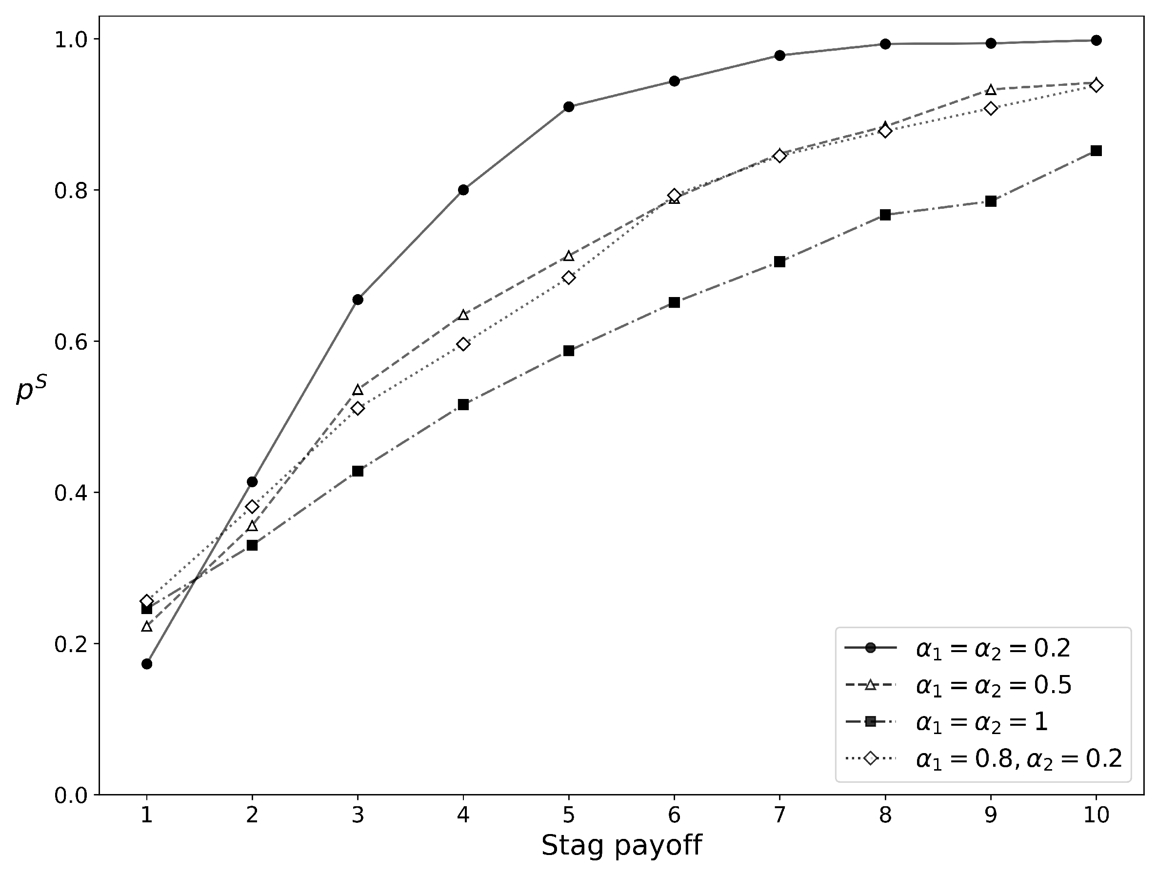
Figure 2 displays the evolution of p S as the Stag’s payoff π S increases for four different scenarios that reflect the interaction between agents with different values of the learning rate α , including the baseline case ( α 1 = α 2 = 1 ). The scenarios were not selected based on any specific criteria but are intended simply to explore different combinations of α , where the agents exhibit increasing values of the learning rate ( 0.2 , 0.5 , 1 ), in addition to a mixed case ( 0.8 , 0.2 ) where agents learn at different speeds. As we have already seen in Section 3.1, as the Stag’s payoff increases, we observe higher values of p S for any combination of α 1 and α 2 . However, the highest values are observed as the learning rate decreases, particularly when both agents exhibit a very low learning rate α , as we can see for α 1 = α 2 = 0.2 . Also in the case of heterogeneous agents, such as in the scenario α 1 = 0.8 and α 2 = 0.2 , where only one of the agents has a low learning rate, we observe higher average values of p S compared to the baseline.
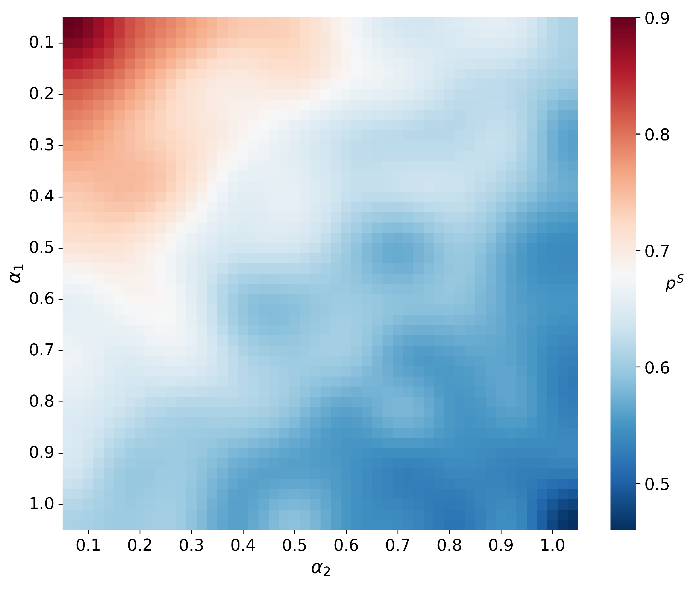
To better understand the underlying dynamics, we can examine Figure 3, which shows the probability of choosing Stag for each combination of the values α 1 and α 2 when π S = 4 . The dark red areas indicate higher values of p S , while the dark blue areas indicate a low probability of coordinating on Stag. As can be clearly seen, the probability p S varies widely depending on the pair of values α 1 and α 2 , ranging from p S 0.5 in the baseline model ( α = 1 ) to p S 0.9 for α 1 = α 2 = 0.1 . As the values of α decrease for both agents, the probability of cooperation increases monotonically. Table 2 lists the simulation parameters employed for the results shown in Figure 3.
The highest value of p S is therefore reached when both agents exhibit the lowest learning rate tested ( α = 0.1 ). In heterogeneous pairs of agents with different α , the presence of a “slow learner” is generally beneficial for cooperation, increasing the overall probability of choosing Stag. For example, in the case where α 1 = 1 , p S tends to increase as the value of α 2 decreases. The results therefore seem to suggest that slower learning benefits cooperation between agents. Gradually updating one’s behavioral rule provides sufficient space to test different strategies and avoid becoming stuck in a strategic stalemate.

3.2.2. Error Probability Effect

In the previous section, we examined the effect of the learning rate on the probability of coordination in Stag, but without considering the possibility of making mistakes. To analyze this different scenario, let us again consider two agents, each endowed with its own probability of making mistakes, μ . For now, let us assume a constant and maximum learning rate α 1 = α 2 = 1 . It is important to emphasize that the results presented do not report the actual choices made by the agents (Stag or Hare), but only the internal probabilities of each agent choosing Stag. For a comparison of actual behavior and internal probabilities, see Appendix B.
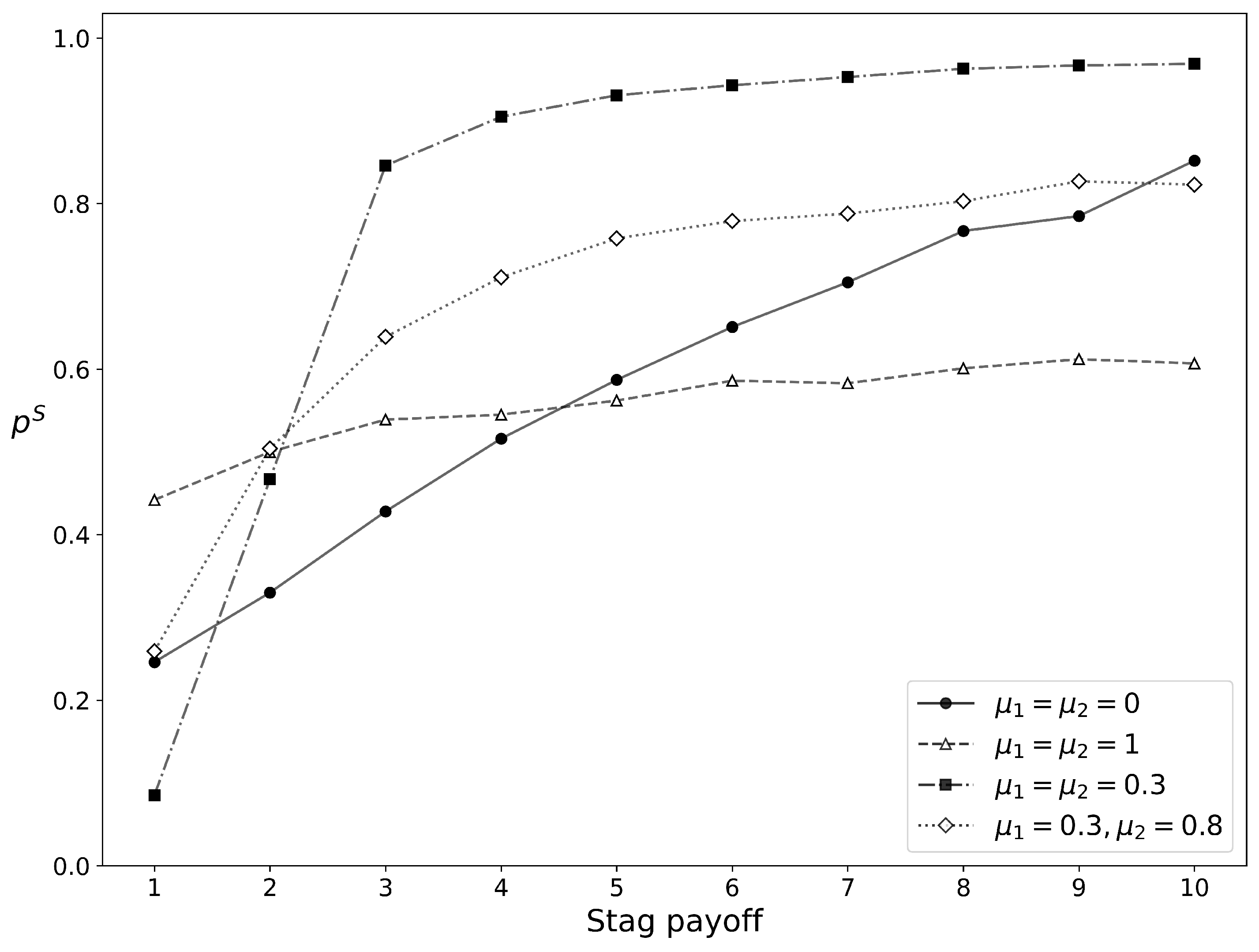
As we can see in Figure 4, the introduction of μ can either increase or decrease the probability of coordinating on Stag p S . Compared to the baseline model ( μ 1 = μ 2 = 0 ), a small probability of making mistakes can be beneficial, as can be observed when μ = 0.3 for both agents. Conversely, high values of μ tend to result in values of p S that are lower than the baseline as the payoff of Stag π S increases. In the case of heterogeneous agents ( μ 1 = 0.3 , μ 2 = 0.8 ), the presence of a single agent with a low probability of making errors is sufficient to offset the negative effect of a high μ , resulting in an overall increase in p S compared to the baseline.
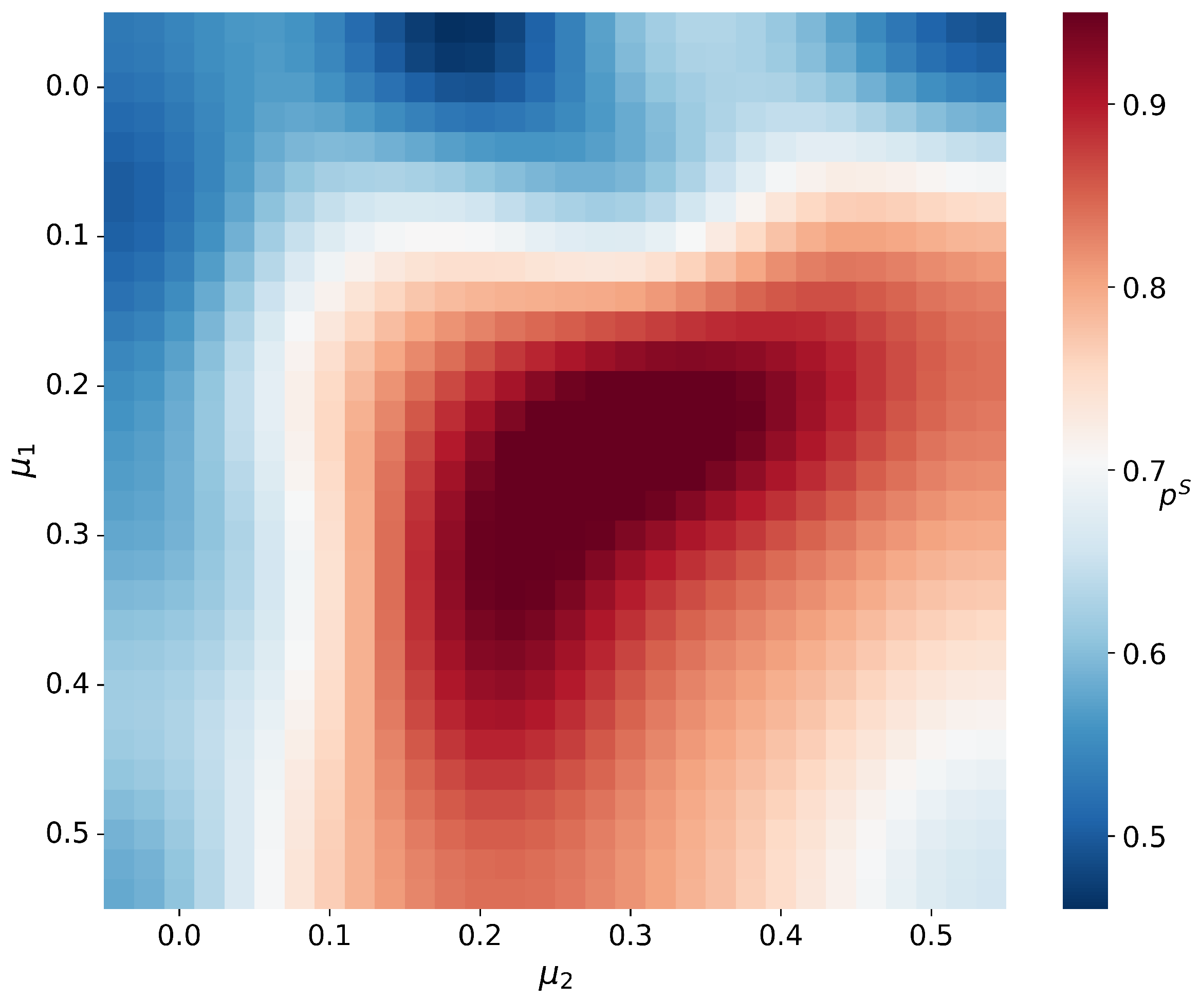
If we examine the values of p S for different combinations of μ 1 and μ 2 ( μ 1 , μ 2 [ 0 , 1 ] ) when π S = 4 (Figure 5), we can see how the probability of choosing Stag initially tends to rise as μ increases (see Table 3 for the list of simulation parameters employed). The maximum point is reached when both agents have a value of μ in the range 0.2–0.3. Moving towards higher values, the probability of cooperating gradually decreases. When the maximum value μ = 1 is reached, the value of p S is close to the case μ = 0 . In this region, high behavioral instability due to frequent mistakes makes any form of learning difficult, if not impossible. Keeping the error probability μ 1 of one of the two agents in the optimal region 0.2–0.3 fixed, we can observe that for increasing values of μ 2 , the probability p S is still relatively high ( p μ 2 = 1 S ∼0.75), compared to the baseline model.
In this scenario, despite rapid learning, the possibility of making mistakes represents another way to experiment with different strategies, with the same positive effects seen in the case of a low learning rate. In fact, even a small chance of making mistakes is enough to allow agents to break through possible strategic deadlocks. In the case of an agent with a high probability of error, this can still be beneficial if the other party exhibits a relatively low probability of errors.

3.2.3. Combined Effect of Learning Rate and Error Probability

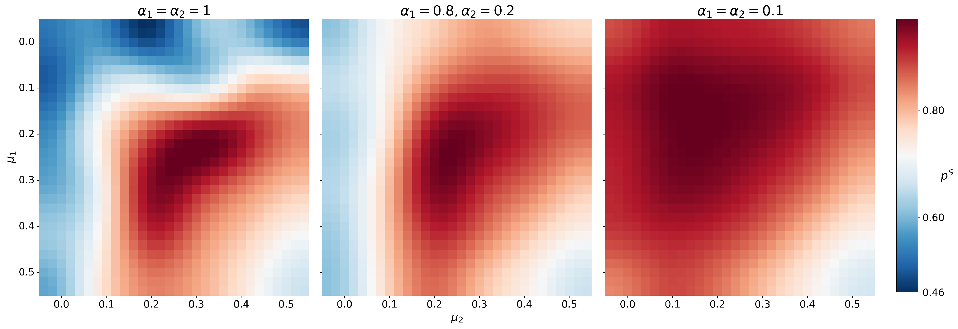
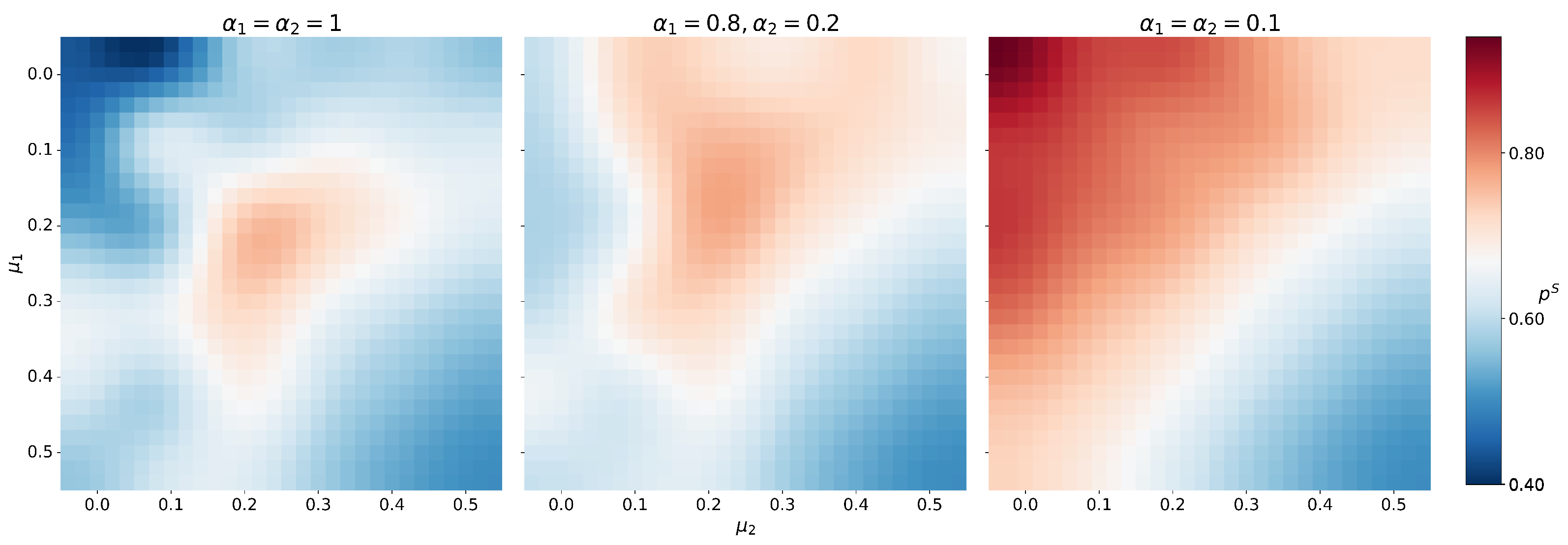
Let’s now consider the joint impact of the learning rate α and the error probability μ on the probability of cooperating p S . Figure 6 shows three different scenarios: for each combination of μ 1 and μ 2 , we assign the agents the maximum ( α 1 = α 2 = 1 ) and minimum ( α 1 = α 2 = 0.1 ) learning rate values, as well as a mixed case ( α 1 = 0.8 , α 2 = 0.2 ).
As seen in the previous section, when the learning rate of both agents is maximum, we observe the smallest probability of choosing Stag; conversely, when α = 0.1 , the value of p S is the highest. On the other hand, the effect of the error μ is non-linear: an error probability between 0.2 and 0.3, even for a single agent, is usually beneficial.
Combining the two factors, we observe how their interplay contributes to widening the region of high coordination (red areas). In particular, as the learning rate decreases, the optimal interval for coordination given by μ tends to widen. From a narrow range of approximately 0.2 μ 0.3 with α 1 = α 2 = 1 , the interval widens significantly, up to approximately 0 μ 0.5 when α 1 = α 2 = 0.1 . We can observe this effect even in the case of heterogeneous agents ( α 1 = 0.8 , α 2 = 0.2 ), where the presence of a single slow learner is capable of extending the positive effect of μ .
These results therefore seem to suggest a specific synergy between the learning rate and the error probability that can promote coordination. While decreasing learning rates tend to increase p S , the noise introduced by μ is beneficial only if limited. However, the detrimental effect of overly frequent errors can be counterbalanced by a gradual learning process, promoting cooperation even in situations where behavior is more erratic.

3.3. Comparison with Experimental Results

In this section, we will compare the results of our simulations with a recent experiment (see Appendix A), where pairs of participants played a computerized version of the SH game. Unlike other experimental designs, players were not provided with any information about the structure and rules of the game, in order to stimulate learning and exploration. During the game, participants were able to observe their partner’s moves, but no communication was possible. In this version of the SH, each player was presented with a horizontal grid, whose two ends represented the Stag and the Hare, and could move to the right or the left to reach one of the two ends. Each move involved a cost in “energy” to be subtracted from their initial endowment, similarly to the mechanism employed in our computational model. Each session consisted of at least 100 rounds. In total, 45 dyads completed the experiment, resulting in 5186 rounds. The payoff matrix used is reported in Table 4.
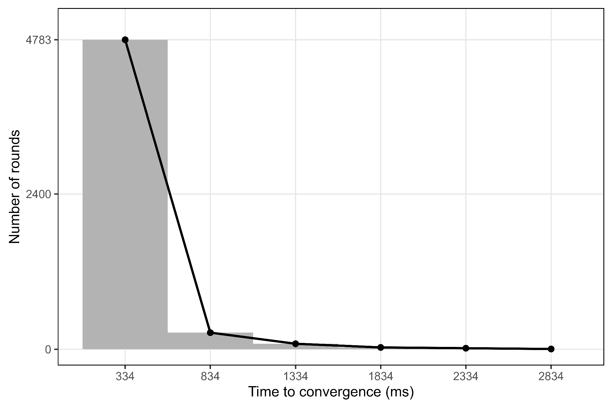
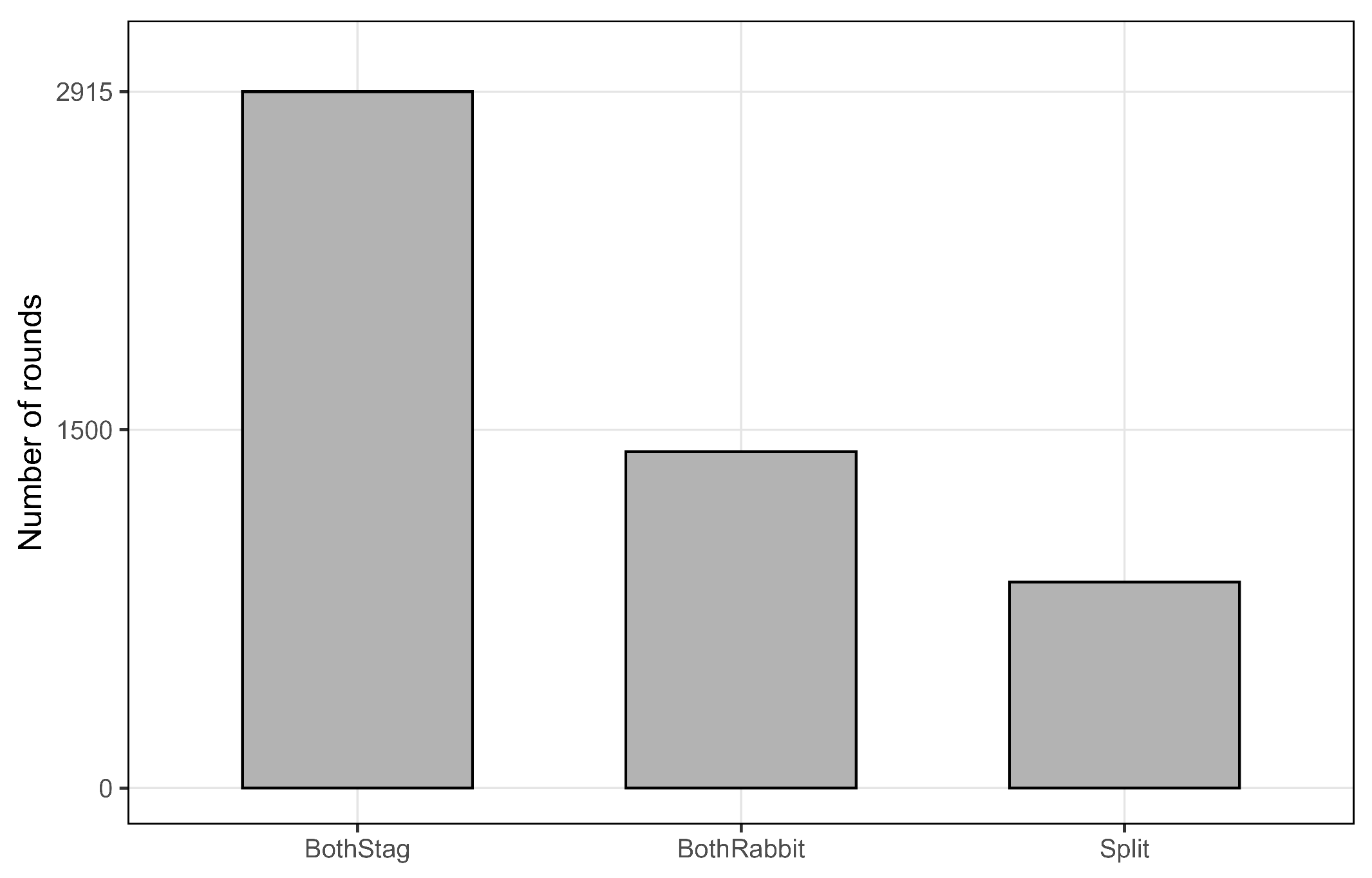
To evaluate the dynamics of cooperation, we analyzed when and how the dyads reached a stable joint strategy within each round. For the purpose of empirical comparison, cooperation is intended as convergence on a strategy. Furthermore, convergence was defined as the first moment within a round when both players simultaneously selected a defined joint state: ( S , S ) (BothStag), ( H , H ) (BothHare), ( S , H ) (Split). For each dyad and round, we identified the earliest move corresponding to a valid joint state and computed the convergence time as the maximum elapsed time between the two participants to account for slower players. Players quickly learned that the ( S , S ) strategy was the most profitable, adopting it most frequently (2915 rounds), followed by the ( H , H ) strategy (1408 rounds) and the least-profitable ( S , H ) strategy (863 rounds). The behavioral results also highlighted a rapid conversion within each round, with a mean convergence time of 334 ms (Figure 7). Most rounds reached a stable configuration within 834 ms, implying early mutual adaptation.
Early convergence suggests that participants rapidly coordinated their strategies, requiring only a few movement corrections. The speed of the players’ actions would seem to suggest a tendency toward a more intuitive and less deliberate decision-making approach, as assumed in our model. Moreover, the predominance of the ( S , S ) state (BothStag) indicates that cooperative balance was not only achievable, but also more stable once reached (Figure 8). Finally, similarly to our computational results, in more than half of the cases, the players were able to coordinate by both choosing Stag. Furthermore, the possibility of observing the opponent’s actions during the game seems to have a very limited effect, justifying a posteriori the simplification made to the simulation model by not allowing the agents to observe each other during the game round.

4. Discussion

In this work, we simulated the learning dynamics of a couple of agents interacting in a Stag-hunt game, where one strategy (Hare) provides a reward independently from the opponent’s choice, while the other one (Stag) guarantees a larger payoff but only if both players adopt it. Therefore, to achieve the best outcome, agents have to learn not only which is the best behavior, but also to coordinate and choose it simultaneously. In order to describe and analyze the dynamics at stake, we considered a very simple model where the agents update their inner probability to choose a given strategy on the basis of the rewards accumulated during the entire interaction when such strategy has been adopted. In a refined version of this model, we tested the effect of agents’ (bounded) cognitive abilities on the fate of the dynamics, i.e., the possibility to learn at a slower rate and to make mistakes, that is, to adopt the opposite strategy selected by applying the learning rule.
Despite the oversimplification of the models, we have been able to reproduce some important features observed in real experiments. In particular, we see that the players always coordinate, that is, they learn that adopting the same behavior is always better (or, at least, not worse) than choosing different strategies. This is in good accordance with the empirical findings described in Section 3.3, where only a small minority of pairs of players were unable to coordinate. These results also appear to be consistent with other experimental findings in the literature: for example, in Van Huyck et al. (1990), dyads formed by the same players over time are able to coordinate to achieve the most efficient outcome.
As shown by the experimental results described in the previous section, in our model, the probability to find the best option (coordinating on Stag) increases with the reward provided by the corresponding strategy. This finding also emerges in some experimental studies on the optimization premium (Battalio et al., 2001) or the salience of the payoff (Silva, 2024), although the literature remains mixed on the role played by payoff differences in the strategies adopted.
Counterintuitively, but not surprisingly, adding a small but not negligible amount of deficiencies to the agents’ behavior helps them to find the best option more efficiently. In fact, for fast-learning and flawless agents, selecting Hare always increases the likelihood of this strategy, regardless of the partner’s behavior, but the same cannot be said for choosing Stag. Therefore, high-performing agents can understand that coordinating on Stag is the most profitable behavior only if both players opt for Stag at the beginning of the interaction, which on average happens with a probability of 1/4 (indeed, the final average probability to choose Stag becomes larger than 1/2 when the reward for mutual Stag is larger than Hare’s reward). The asymmetry inherent in the SH game and its payoff structure can therefore penalize the best-performing agents, who may remain stuck in a less remunerative position. Therefore, letting the players “make mistakes” allows them to explore more strategic options and understand if there are better configurations, given that this probability to make such mistakes is not too high in order to avoid random behavior. This result appears to be consistent with previous studies in the literature, in which agents equipped with simpler strategic mechanisms, such as imitation (Weidenholzer, 2010), random walks (Macy & Flache, 2002), or the use of heuristics (Belloc et al., 2019), are able to coordinate their actions to achieve the most efficient outcome.
The main limit of the models presented is that they are classical game-theoretical models where players have to decide instantaneously their strategy with no information about the opponent’s intentions. In the experimental setting described in Section 3.3, each player decided whether to choose Stag or Hare while being able to observe the direction taken by their partner. Information about the behavior of other players can certainly have an impact on decision-making processes, in addition to the learning and evaluation abilities of each individual player that we investigated in this work. For this reason, we believe that future extensions of this model should integrate the role of such information and different game mechanics, such as the absence of simultaneous choices, in the decision-making processes of agents. Furthermore, other extensions could consider multi-strategy frameworks, where agents are not limited to two strategies but have the option, for example, to not play. Finally, in this study, we assumed a constant and uniform error probability and a learning mechanism separate from the former, finding that a combination of low learning rates and low error probabilities promotes coordination toward the social optimum. However, as suggested by some empirical studies on coordination (Bilancini et al., 2021; Mäs & Nax, 2016), human error does not appear to be constant but rather sensitive to changes in payoffs, expected costs, and past successes, outlining a more complex and structured dynamic. Future extensions could therefore integrate the error probability and learning into a single adaptive mechanism, allowing agents to change their propensity to make errors through experience.

Author Contributions

Conceptualization, R.M. and D.V.; methodology, R.M. and D.V.; software, R.M. and D.V.; formal analysis, R.M., D.V. and T.J.C.; investigation, R.M., D.V. and T.J.C.; data curation, R.M. and T.J.C.; writing—original draft preparation, R.M., D.V. and T.J.C.; writing—review and editing, R.M., D.V., T.J.C., A.G. and F.B.; supervision, D.V., A.G. and F.B.; project administration, R.M., D.V. and T.J.C.; funding acquisition, D.V., A.G. and F.B. All authors have read and agreed to the published version of the manuscript.

Funding

This research was funded by the European Italian Ministry of Research through the PRIN-PNRR project COBRA, grant number P2022JZRWS.

Informed Consent Statement

Informed consent was obtained from all subjects involved in the study.

Data Availability Statement

The data used for this research have been generated by simulations, whose codes can be found at https://github.com/p0lynmial/COBRA-Project-Inefficient-learning-leads-to-efficient-coordination-, accessed on 18 June 2026.

Acknowledgments

D. V., T. C. and A. G. thank Ruck Thawonmas and his group at Ritsumeikan University, Ibaraki (Japan), for the useful and inspiring discussions about this research during their visit at Ritsumeikan in April–May 2025.

Conflicts of Interest

The authors declare no conflicts of interest.

Abbreviations

The following abbreviations are used in this manuscript:
SHStag-hunt game
α Learning rate
μ Error probability
p S Probability that agents coordinate on Stag
π S Stag’s payoff

Appendix A

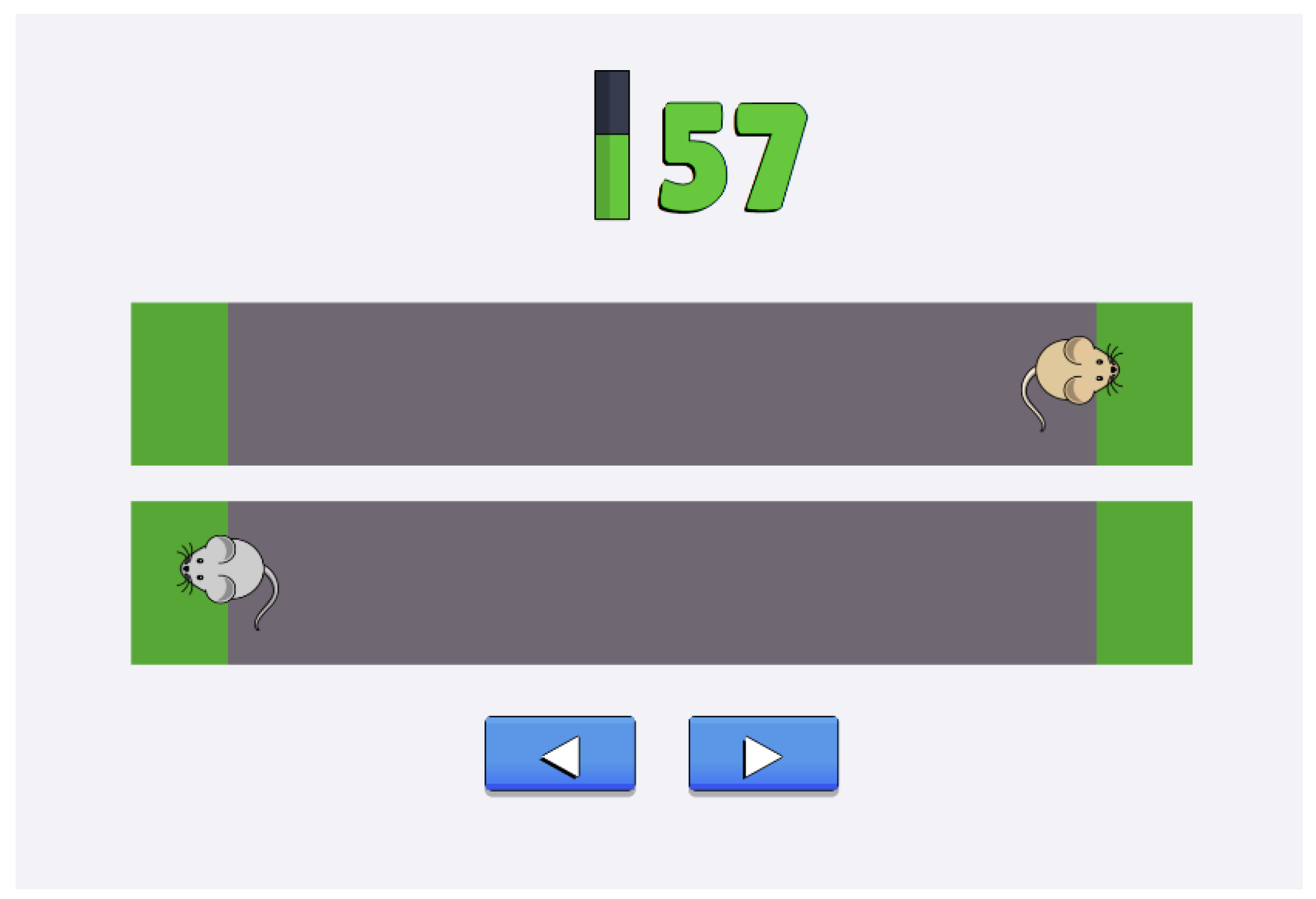
The experimental task consisted of a spatially extended and repeated Stag-hunt game. Two players, represented by two mice, played multiple rounds in a shared virtual environment. At the beginning of each round, both players started from a common location and had to move toward one of two possible reward areas: the Stag or the Hare. Each round ended once both players reached a reward area. The reward locations were 20 steps away from the starting point and each step reduced the player’s available energy. This made movement costly and required players to commit to a direction during the round. The players could not communicate with each other. Therefore, they could not explicitly plan a joint strategy before or during the round. Instead, they had to rely only on the other player’s visible movement. The rewards were also not explicitly indicated at the beginning, so players had to explore the environment and learn the positions and consequences of the Stag and Hare across repeated rounds. This design transformed the classical Stag hunt into a dynamic coordination task. Rather than making a single isolated choice, players had to learn the environment, monitor their partner’s movement, manage their own energy and decide whether to coordinate on the risky cooperative option or pursue the safer individual option as can be seen in Figure A1.
This experiment has been accomplished within Project COBRA (see Funding), whose complete results will be published soon.
Figure A1. Experimental interface of the virtual SH game as seen by the test subject. Using the arrows at the bottom, the player can choose which direction to take, whilst the position and movements of both players are displayed in the center. The number at the top indicates the player’s remaining energy (payoff).
Games 17 00039 g0a1

Appendix B

In Section 3.2.2 and Section 3.2.3, we analyzed the impact of the error probability μ on the probability p S that agents will choose Stag, as well as the combined effect of μ with different learning rates α . As we have seen, a moderate probability of making errors proved to be beneficial: by experimenting with different strategies, the agents tend to coordinate more easily on the social optimum, namely Stag. This effect is accentuated when both agents exhibit low learning rates, as shown in Figure 6. However, these results refer exclusively to the probability p S , which we can interpret as the agent’s intention or the outcome of its evaluation, and do not reflect the actual actions taken by the players, which are instead shown in Figure A2.
Figure A2. Stag selection frequency f S for different combinations of { μ 1 , μ 2 } and { α 1 , α 2 }, with Stag’s payoff π S = 4 . Starting from the left, the graph displays the results for the scenarios with maximum learning rates ( α 1 = α 2 = 1 ), mixed learning rates ( α 1 = 0.8 , α 2 = 0.2 ), and minimum learning rates ( α 1 = α 2 = 0.1 ).
Games 17 00039 g0a2
As expected, the frequency of Stag selection f S follows a trend similar to p S , but with generally lower values. While μ promotes learning among agents, excessive noise can interfere with the adoption of the optimal choice. The exploration of the strategies induced by μ allows agents to understand the benefits of coordinating on Stag, but at the same time, it can prevent the adoption of this choice.

Appendix C

In Section 3, we reported the average probability p S that agents 1 and 2 will choose Stag. As we have seen, for low learning rates and low error probabilities, players are more likely to coordinate on Stag. Since the aggregated results do not show the individual probabilities for each agent, Table A1 reports the average absolute difference in the final probabilities across the tested scenarios. The numerical values provided allow us to understand how the probabilities p 1 S and p 2 S diverge, depending on the chosen parameters. In general, the deviation is small and tends to increase when the agents’ error probabilities are asymmetric and μ takes on high values. The error probability also affects the variability of these results, which increases as μ increases. However, it is important to note that the learning rate can mitigate this effect. In fact, as the learning rate decreases, the variability also tends to decrease. This effect is due to the agents’ reduced responsiveness to the fluctuations induced by the error probability. A more gradual learning process, as in the case of α 1 = α 2 = 0.1 , would therefore make the agents more resilient to inconsistent results caused by errors.
Table A1. The table shows the average absolute difference between the final probabilities of choosing Stag for the two agents, p 1 S and p 2 S . The standard deviations are shown in parentheses. The results show the average of 10 3 generations for each pair of values μ 1 and μ 2 and for the three scenarios defined by the different learning rate values: (i) α 1 = α 2 = 1 , (ii) α 1 = 0.8 , α 2 = 1 , (iii) α 1 = α 2 = 0.1 .
α 1 = α 2 = 1
μ 00.10.20.30.40.5
00.0230.0020.0110.0350.0790.129
(0.149)(0.006)(0.026)(0.059)(0.104)(0.138)
0.10.0020.0050.0220.0740.1670.235
(0.007)(0.009)(0.030)(0.075)(0.134)(0.146)
0.20.0110.0230.0500.0680.1310.195
(0.024)(0.030)(0.075)(0.075)(0.113)(0.145)
0.30.0340.0740.0670.0890.1380.179
(0.060)(0.077)(0.071)(0.083)(0.111)(0.131)
0.40.0790.1570.1350.1360.1560.167
(0.108)(0.125)(0.117)(0.110)(0.117)(0.130)
0.50.1320.2440.2130.1770.1660.162
(0.142)(0.147)(0.147)(0.134)(0.126)(0.121)
α 1 = 0.8 , α 2 = 0.2
μ 00.10.20.30.40.5
00.0200.0200.0360.0660.1230.185
(0.110)(0.049)(0.045)(0.042)(0.053)(0.066)
0.10.0060.0050.0190.0690.1530.229
(0.050)(0.006)(0.013)(0.037)(0.070)(0.074)
0.20.0180.0200.0310.0530.1260.204
(0.025)(0.026)(0.040)(0.034)(0.060)(0.071)
0.30.0500.0640.0590.0610.1020.162
(0.056)(0.062)(0.064)(0.052)(0.069)(0.088)
0.40.1140.1370.1330.1060.1010.124
(0.100)(0.104)(0.103)(0.089)(0.080)(0.084)
0.50.1730.2100.2080.1610.1220.114
(0.122)(0.123)(0.131)(0.116)(0.097)(0.084)
α 1 = α 2 = 0.1
μ 00.10.20.30.40.5
00.0160.0300.0640.1030.1400.189
(0.065)(0.062)(0.061)(0.059)(0.063)(0.059)
0.10.0340.0220.0420.0840.1260.182
(0.080)(0.033)(0.037)(0.044)(0.047)(0.063)
0.20.0650.0440.0390.0600.0990.142
(0.070)(0.039)(0.036)(0.043)(0.050)(0.059)
0.30.1050.0840.0620.0500.0650.088
(0.067)(0.044)(0.044)(0.035)(0.044)(0.052)
0.40.1390.1260.1000.0640.0500.051
(0.061)(0.046)(0.052)(0.044)(0.036)(0.038)
0.50.1940.1810.1420.0860.0540.045
(0.066)(0.062)(0.061)(0.049)(0.039)(0.032)

References

  1. Arad, A., & Rubinstein, A. (2012). The 11–20 money request game: A level-k reasoning study. American Economic Review, 102(7), 3561–3573. [Google Scholar] [CrossRef] [Scilit]
  2. Axelrod, R. (1981). The emergence of cooperation among egoists. American Political Science Review, 75(2), 306–318. [Google Scholar] [CrossRef] [Scilit]
  3. Bardsley, N., Mehta, J., Starmer, C., & Sugden, R. (2010). Explaining focal points: Cognitive hierarchy theory versus team reasoning. The Economic Journal, 120(543), 40–79. [Google Scholar]
  4. Battalio, R., Samuelson, L., & Van Huyck, J. (2001). Optimization incentives and coordination failure in laboratory stag hunt games. Econometrica, 69(3), 749–764. [Google Scholar] [CrossRef] [Scilit]
  5. Belloc, M., Bilancini, E., Boncinelli, L., & D’Alessandro, S. (2019). Intuition and deliberation in the stag hunt game. Scientific Reports, 9(1), 14833. [Google Scholar] [CrossRef] [Scilit] [PubMed]
  6. Bilancini, E., Boncinelli, L., & Nax, H. H. (2021). What noise matters? Experimental evidence for stochastic deviations in social norms. Journal of Behavioral and Experimental Economics, 90, 101626. [Google Scholar] [CrossRef] [Scilit]
  7. Camerer, C. F., Ho, T.-H., & Chong, J.-K. (2004). A cognitive hierarchy model of games. The Quarterly Journal of Economics, 119(3), 861–898. [Google Scholar] [CrossRef] [Scilit]
  8. Challet, D., & Zhang, Y.-C. (1997). Emergence of cooperation and organization in an evolutionary game. Physica A: Statistical Mechanics and Its Applications, 246(3–4), 407–418. [Google Scholar] [CrossRef] [Scilit]
  9. Chen, R., & Chen, Y. (2011). The potential of social identity for equilibrium selection. American Economic Review, 101(6), 2562–2589. [Google Scholar] [CrossRef] [Scilit]
  10. Cooper, D. J., & Weber, R. A. (2020). Recent advances in experimental coordination games. In Handbook of experimental game theory (pp. 149–183). Edward Elgar Publishing. [Google Scholar] [CrossRef] [Scilit]
  11. De Kwaadsteniet, E. W., & Van Dijk, E. (2010). Social status as a cue for tacit coordination. Journal of Experimental Social Psychology, 46(3), 515–524. [Google Scholar] [CrossRef] [Scilit]
  12. Devetag, G., & Ortmann, A. (2014). Chapter 16—Solving coordination problems experimentally. In M. Webster, & J. Sell (Eds.), Laboratory experiments in the social sciences (2nd ed., pp. 357–384). Academic Press. Available online: https://www.sciencedirect.com/science/article/pii/B9780124046818000169 (accessed on 18 June 2026).
  13. Engelmann, D., & Normann, H.-T. (2010). Maximum effort in the minimum-effort game. Experimental Economics, 13(3), 249–259. [Google Scholar] [CrossRef] [Scilit]
  14. Fallucchi, F., & Nosenzo, D. (2022). The coordinating power of social norms. Experimental Economics, 25(1), 1–25. [Google Scholar] [CrossRef] [Scilit]
  15. Flache, A., & Macy, M. W. (2002). Stochastic collusion and the power law of learning: A general reinforcement learning model of cooperation. Journal of Conflict Resolution, 46(5), 629–653. [Google Scholar] [CrossRef] [Scilit]
  16. Hofbauer, J., & Sigmund, K. (1998). Evolutionary games and population dynamics. Cambridge University Press. [Google Scholar]
  17. Krupka, E. L., Weber, R., Crosno, R. T., & Hoover, H. (2022). “When in Rome”: Identifying social norms usingcoordination games. Judgment and Decision Making, 17(2), 263–283. [Google Scholar] [CrossRef] [Scilit]
  18. Krupka, E. L., & Weber, R. A. (2013). Identifying social norms using coordination games: Why does dictator game sharing vary? Journal of the European Economic Association, 11(3), 495–524. [Google Scholar] [CrossRef] [Scilit]
  19. Macy, M. W., & Flache, A. (2002). Learning dynamics in social dilemmas. Proceedings of the National Academy of Sciences of the United States of America, 99(Suppl. S3), 7229–7236. [Google Scholar] [CrossRef] [Scilit] [PubMed]
  20. Mäs, M., & Nax, H. H. (2016). A behavioral study of “noise” in coordination games. Journal of Economic Theory, 162, 195–208. [Google Scholar] [CrossRef] [Scilit]
  21. Nagel, R. (1995). Unraveling in guessing games: An experimental study. The American Economic Review, 85(5), 1313–1326. [Google Scholar]
  22. Raducha, T., & San Miguel, M. (2022). Coordination and equilibrium selection in games: The role of local effects. Scientific Reports, 12(1), 3373. [Google Scholar] [CrossRef] [Scilit] [PubMed]
  23. Roca, C. P., Cuesta, J. A., & Sánchez, A. (2009a). Effect of spatial structure on the evolution of cooperation. Physical Review E—Statistical, Nonlinear, and Soft Matter Physics, 80(4), 046106. [Google Scholar] [CrossRef] [Scilit]
  24. Roca, C. P., Cuesta, J. A., & Sánchez, A. (2009b). Evolutionary game theory: Temporal and spatial effects beyond replicator dynamics. Physics of Life Reviews, 6(4), 208–249. [Google Scholar] [CrossRef] [Scilit]
  25. Roth, A. E., & Erev, I. (1995). Learning in extensive-form games: Experimental data and simple dynamic models in the intermediate term. Games and Economic Behavior, 8(1), 164–212. [Google Scholar] [CrossRef] [Scilit]
  26. Rubinstein, A. (2016). A typology of players: Between instinctive and contemplative. The Quarterly Journal of Economics, 131(2), 859–890. [Google Scholar] [CrossRef] [Scilit]
  27. Silva, R. (2024). Coordination in stag hunt games. Journal of Behavioral and Experimental Economics, 113, 102290. [Google Scholar] [CrossRef] [Scilit]
  28. Skyrms, B. (2001). The stag hunt (Vol. 75, No. 2, pp. 31–41). American Philosophical Association. [Google Scholar]
  29. Skyrms, B. (2004). The stag hunt and the evolution of social structure. Cambridge University Press. [Google Scholar]
  30. Stahl, D. O., & Wilson, P. W. (1995). On players’ models of other players: Theory and experimental evidence. Games and Economic Behavior, 10(1), 218–254. [Google Scholar] [CrossRef] [Scilit]
  31. Tomassini, M., & Pestelacci, E. (2010). Coordination games on dynamical networks. Games, 1(3), 242–261. [Google Scholar] [CrossRef] [Scilit]
  32. Van Huyck, J. B., Battalio, R. C., & Beil, R. O. (1990). Tacit coordination games, strategic uncertainty, and coordination failure. The American Economic Review, 80(1), 234–248. [Google Scholar]
  33. Vilone, D., Realpe-Gómez, J., & Andrighetto, G. (2021). Evolutionary advantages of turning points in human cooperative behaviour. PLoS ONE, 16(2), e0246278. [Google Scholar] [CrossRef] [Scilit] [PubMed]
  34. Weidenholzer, S. (2010). Coordination games and local interactions: A survey of the game theoretic literature. Games, 1(4), 551–585. [Google Scholar] [CrossRef] [Scilit]
Figure 1. Average probability to adopt the Stag strategy by the two players. Since, in each simulated experiment, agents end up choosing the same strategy with probability p i S = 1 , this graph shows the probability that a single realization ends up with players going for the Stag.
Games 17 00039 g001
Figure 2. Average probability to adopt Stag strategy for different values of the Stag’s payoff. The graph shows the results for three different combinations of α 1 and α 2 , in addition to the baseline model ( α 1 = α 2 = 1), for increasing values of the Stag payoff ( π S [ 1 , 10 ] ) and no error probability ( μ 1 = μ 2 = 0 ).
Games 17 00039 g002
Figure 3. Average probability to adopt the Stag strategy for different combinations of the learning rates α 1 and α 2 . The graph displays the values of p S as α 1 and α 2 vary for π S = 4 and μ 1 = μ 2 = 0 . When both agents exhibit a very low learning rate, we observe the highest values of p S (dark red area); conversely, when the learning rate is high, p S tends to decrease (dark blue areas).
Games 17 00039 g003
Figure 4. Average probability to adopt Stag strategy for different values of the Stag’s payoff. The graph shows the results for three different combinations of μ 1 and μ 2 , in addition to the baseline model ( μ 1 = μ 2 = 0 ), for increasing values of the Stag payoff ( π S [ 1 , 10 ] ) and fixed learning rates ( α 1 = α 2 = 1 ).
Games 17 00039 g004
Figure 5. Average probability to adopt the Stag strategy for different combinations of the error probabilities μ 1 and μ 2 . The graph shows the results for π S = 4 and α 1 = α 2 = 1 . The red areas indicate high values of p S , while the blue areas indicate a low probability of coordinating on Stag.
Games 17 00039 g005
Figure 6. Average probability to adopt the Stag strategy for different combinations of { μ 1 , μ 2 } and { α 1 , α 2 }, with Stag’s payoff π S = 4 . Starting from the left, the graph displays the results for the scenarios with maximum learning rates ( α 1 = α 2 = 1 ), mixed learning rates ( α 1 = 0.8 , α 2 = 0.2 ), and minimum learning rates ( α 1 = α 2 = 0.1 ).
Games 17 00039 g006
Figure 7. Convergence times observed in the experimental SH. In the majority of rounds played (92%), the experimental subjects tended to quickly converge on a stable configuration.
Games 17 00039 g007
Figure 8. Frequency of joint states at first convergence. In more than half of the rounds played (56%), the players managed to coordinate on the social optimum (S,S). The second most frequent configuration (27%) was (H,H), followed by the least efficient one (S,H).
Games 17 00039 g008
Table 1. Payoff matrix P ^ for the player i. The parameter r indicates the payoff obtained by choosing Hare, while ϵ is the additional payoff relative to Hare, obtained by both agents when they coordinate on Stag.
StagHare
Stag r + ε 0
Harerr
Table 2. Simulation parameters. The table lists the learning rates ( α 1 , α 2 ) and error probabilities ( μ 1 , μ 2 ) of agents 1 and 2, the Stag’s payoff ( π S ), the maximum number of iterations (t) if convergence is not achieved, and the total number of generations (T).
α 1 α 2 μ 1 μ 2 π S tT
( 0 , 1 ] ( 0 , 1 ] 004 10 5 10 3
Table 3. Simulation parameters. The table lists the learning rates ( α 1 , α 2 ) and error probabilities ( μ 1 , μ 2 ) of agents 1 and 2, the Stag’s payoff ( π S ), the maximum number of iterations (t) if convergence is not achieved, and the total number of generations (T).
α 1 α 2 μ 1 μ 2 π S tT
11 [ 0 , 0.5 ] [ 0 , 0.5 ] 4 10 5 10 3
Table 4. Payoff matrix employed in the experimental setting. Players were not informed about the potential payouts associated with the two actions, i.e., left and right movements.
StagHare
Stag ( 4 a , 4 a ) ( 0 , a )
Hare ( a , 0 ) ( a , a )
Disclaimer/Publisher’s Note: The statements, opinions and data contained in all publications are solely those of the individual author(s) and contributor(s) and not of MDPI and/or the editor(s). MDPI and/or the editor(s) disclaim responsibility for any injury to people or property resulting from any ideas, methods, instructions or products referred to in the content.