A Dynamic Game Model to Estimate Market Competitiveness: An Application to the Chinese Retail Oil Market

Abstract

This paper develops a dynamic game-theoretic model to evaluate market competitiveness in industries characterized by price competition and adjustment stickiness. We extend the dynamic oligopoly framework for estimating market competitiveness in the literature from a quantity-setting to a price-setting context with differentiated goods. By deriving the subgame perfect equilibrium in a linear-quadratic structure, we utilize an index analogous to the price conjectural variation to measure market competitiveness with differentiated goods. The model is applied to the Chinese retail oil market, and we find that the Chinese retail oil market, particularly dominated by two state firms, exhibits characteristics close to a collusive benchmark within the maintained model. The dynamic game model provides a tractable analytical tool for antitrust authorities to monitor strategic coordination in dynamic environments where price transparency or regulation may facilitate tacit coordination of pricing behavior to a high degree.

1. Introduction

Energy market reform is taking place in many emerging countries. For instance, the retail oil market in China has witnessed increased competition in recent years. However, the two largest national oil companies—PetroChina and Sinopec—still dominate the market (Zhang et al., 2020). This raises concerns about potential market power. Meanwhile, the potential collusion or market competitiveness in retail oil markets is a great concern all over the world. The unique characteristics inherent to the retail oil (gasoline or diesel) market make it a central concern in the study of collusion due to the prevalence of price transparency in the market (Eckert & West, 2005; Byrne & de Roos, 2019), which helps identify deviations and facilitate collusion stability.

On the other hand, oil firms may have concerns for price adjustment, as emphasized by Davis and Hamilton (2004). Several factors can contribute to the reluctance of firms for adjustment. For instance, if a firm is unsure whether competitors will adjust their prices, it may hesitate to do so itself. This reluctance to be the first mover can create a situation where prices remain sticky. In addition, a firm may encounter an invisible cost, manifesting as the apprehension of adverse responses from government (especially in a regulated market like China) and customers for price changes (e.g., Borenstein et al., 1997; Douglas & Herrera, 2010). Consequently, the price stickiness should also be considered when modeling the pricing behavior of oil firms.

This paper develops a dynamic game model that estimates market competitiveness within an industry characterized by price competition and the presence of price stickiness. Building upon the dynamic oligopoly model established by Karp and Perloff (1989), which employs an index akin to conjectural variation to gauge competitiveness across diverse game scenarios (collusive, price-taking, and Nash–Cournot models) in the rice export market, we extend this framework to accommodate price competition. In our model, market players engage in price competition with stickiness, and therefore we utilize an index akin to the price conjectural variation proposed by Liang (1989), to gauge market competitiveness within the context of differentiated goods.

Many studies have explored price competition and coordination in the retail oil market, including works by Borenstein and Shepard (1996) on the US gasoline market, Eckert and West (2005) on the Canadian (Vancouver) market, Byrne and de Roos (2019) on the Australian (Perth) market, and Zhang et al. (2020) on the Chinese market, among others. These studies have documented a range of dynamic competitive behaviors using high-frequency, station-level price data. A first strand of work identifies Edgeworth price cycles as a common feature in concentrated gasoline markets, where firms repeatedly undercut and then restore prices in a non-stationary pattern (e.g., Noel, 2007; M. Lewis & Noel, 2011). A second strand shows that retail fuel prices often exhibit sticky or asymmetric responses to wholesale cost shocks, with retail prices adjusting more slowly when costs fall than when they rise—an empirical pattern widely interpreted as reflecting market power or coordination (Peltzman, 2000; Radchenko, 2005; Galeotti et al., 2003; Xu et al., 2024). A third strand directly examines tacit coordination, showing that repeated interactions and demand predictability can facilitate collusive price adjustments even without explicit communication (Byrne & de Roos, 2019; Zhang et al., 2020). For example, Byrne and de Roos (2019) demonstrate that leading gasoline firms rely on price leadership and targeted price changes to generate focal pricing benchmarks that facilitate coordination, reduce competitive intensity, and improve retail profitability. Zhang et al. (2020) show that regulated price ceilings in China can serve as focal points that help sustain near-uniform retail prices.

However, an important gap remains in the literature. Existing studies on retail oil markets have documented price cycles, asymmetric adjustment, price leadership, and near-uniform pricing, but they do not provide a unified structural framework that can distinguish whether observed price alignment reflects market power, dynamic adjustment frictions, focal regulatory constraints, or a stronger degree of strategic internalization by firms (Borenstein & Shepard, 1996; Eckert & West, 2005; Noel, 2007; Byrne & de Roos, 2019; Zhang et al., 2020). At the same time, the classic conduct parameter literature is highly useful for interpreting market behavior, but it is largely static and therefore does not explicitly incorporate lagged pricing, state dependence, or price stickiness in posted-price markets (Bresnahan, 1982; Lau, 1982; Liang, 1989). This leaves an unresolved question for concentrated price-setting industries: how should market conduct be interpreted when firms compete through prices, observe each other repeatedly, and adjust only gradually over time?

This paper makes three contributions to the literature. First, the model clarifies what existing frameworks cannot cleanly address: distinguishing persistent price alignment driven by dynamic adjustment frictions and focal institutional constraints from stronger strategic internalization of the rival’s payoff. In static settings, similar prices may be read as evidence of coordination, but in a market with sticky prices and repeated interaction, such similarity in observed prices may instead reflect inherited state variables and gradual adjustment (Borenstein & Shepard, 1996; Davis & Hamilton, 2004; Douglas & Herrera, 2010). Our framework brings these forces into the same structural system.

Second, we show that conduct in posted-price markets is not identified by synchronization per se, but by the joint configuration of demand substitutability, own-price persistence, rival-price response, and continuation values in a dynamic equilibrium. In that sense, the conduct index is not the only contribution; rather, it is the summary statistic emerging from this broader theoretical result about how dynamic pricing behavior should be interpreted in transparent and frictional markets. This logic situates the paper relative to dynamic collusion theory and modern empirical studies of coordinated pricing (Green & Porter, 1984; Rotemberg & Saloner, 1986; Byrne & de Roos, 2019).

Third, our empirical contribution differs from the existing retail fuel literature. Byrne and de Roos (2019) provide rich evidence on coordinated pricing and equilibrium transitions in retail gasoline markets, while Zhang et al. (2020) document strong price uniformity in the Chinese gasoline market under price regulation. In contrast, our paper does not stop at describing price comovement or uniformity. Instead, we estimate a structural conduct parameter for the Chinese retail oil market within a dynamic model that explicitly accounts for price stickiness and strategic persistence. This provides a tractable way to quantify market conduct in a concentrated and regulated market and adds a structural measure to a literature that has often relied on descriptive or reduced-form evidence.

The rest of this paper is organized as follows. Section 2 describes the dynamic price competition by incorporating the market competitiveness measure. Section 3 presents the analytical solution of the model. The application of our model to the Chinese retail oil market is presented in Section 4. Finally, conclusions are summarized in Section 5.

2. The Dynamic Game of Price Competition

Our game model with dynamic price competition is flexible enough to nest the possibility that the players (Firm 1 and Firm 2) act like price takers, colluding, or oligopolistic firms (prices as the strategic variables). Suppose that both firms are engaged in the retail sale of oil to consumers. These consumers perceive the retail oil (gasoline or diesel) from each firm as differentiated goods denoted by $i$, possibly due to factors such as branding. Assume the demand for good $i$ is:

$$Q_{it}={\alpha }_{it}-{\theta }_i{p}_{it}+{\eta }_i{p}_{jt}$$

(1)

where $p_{it}$ is the price of firm $i$ in time period $t$. The marginal cost of production is denoted as $c_{it}$ for firm $i$. At the same time, there exists price stickiness, which is represented by:

$$C(u_{it})=({\gamma }_i+{\displaystyle \frac{{\delta }_i}{2}}{u}_{it})u_{it}$$

(2)

where $u_{it}=p_{it}-p_{i,t-1}$ is the adjustment of the price in time $t$ (relative to the period $t-1$). The parameter ${\delta }_i$ in Equation (2) represents the quadratic component of the adjustment cost, which mathematically captures the ‘price stickiness’ observed in the market. Specifically, in the context of the retail oil market, a high value of ${\delta }_i$ reflects a firm’s apprehension regarding adverse responses from the government or customers when prices deviate from established norms.

Firm $i$ chooses prices to maximize the present discounted value of net benefits:

$${\displaystyle \sum _{t=1}^{\infty }}{\beta }^{t-1}[(p_{it}-c_{it})({\alpha }_{it}-{\theta }_i{p}_{it}+{\eta }_i{p}_{jt})-({\gamma }_i+{\displaystyle \frac{{\delta }_i}{2}}{u}_{it})u_{it}]$$

where $\beta$ is the discount factor. Recursively, one can write the optimization problem of firm $i$ in period t as:

$$J_i(p_{i,t-1},p_{j,t-1})=\underset{u_{it}}{\mathrm{m}\mathrm{a}\mathrm{x}}[(p_{it}-c_{it})({\alpha }_{it}-{\theta }_i{p}_{it}+{\eta }_i{p}_{jt})-({\gamma }_i+{\displaystyle \frac{{\delta }_i}{2}}{u}_{it})u_{it}+\beta J_i(p_{it},p_{jt})]$$

(3)

where we have $p_{it}=p_{i,t-1}+u_{it}$ and $J_i(·)$ is the value function for player $i$. This exhibits the dynamic nature of competition, where the pricing strategy of each firm is contingent upon the prices set in the previous period.

The first-order condition to Equation (3) yields,

$$\begin{array}{c}({\alpha }_{it}-\theta p_{it}+\eta p_{jt})+(p_{it}-c_{it})(-{\theta }_i+{\eta }_i{v}_i)\\ -[{\gamma }_i+\delta (p_{it}-p_{i,t-1})]+\beta [{\displaystyle \frac{\partial J_i(p_{it},p_{jt})}{\partial p_{it}}}+{\displaystyle \frac{\partial J_i(p_{it},p_{jt})}{\partial p_{jt}}}{v}_i]=0\end{array}$$

(4)

where $v_i=d{p}_j/d{p}_i$ is the price conjectural variation analogous to that used in Liang (1989), which describes how firm $i$ perceives the response of firm $j$’s price $p_j$ to its own pricing decision $p_i$. The conjectural variation term reflects how strongly firm i expects firm j to adjust its price in response to a change in firm i’s price. A higher value implies a stronger expected strategic response and therefore a higher degree of coordinated pricing behavior within the model. For a symmetric duopoly market, we would have $v=0$ for independent pricing (oligopolistic pricing); $v=-1$ for competitive market; and $v=1$ for a collusive (cooperative) market (Liang, 1989).

3. Analytical Solution of the Model

The dynamic price competition model developed above can be solved analytically. Following Karp and Perloff (1989), we assume the symmetry between firms, and thus denote $\theta \equiv {\theta }_i={\theta }_j$, $\eta \equiv {\eta }_i={\eta }_j$, ${\gamma \equiv \gamma }_i={\gamma }_j$, ${\delta \equiv \delta }_i={\delta }_j$. Due to the linear-quadratic structure of the problem, one can conjecture the value function of the firm:

$$J_i(p_i,p_j)=a_i+d_o{p}_i+d_r{p}_j+{\displaystyle \frac{1}{2}}{m}_o{p_i}^2+{\displaystyle \frac{1}{2}}{m}_r{p_j}^2+m_x{p}_i{p}_j$$

Plugging the value function into the first-order condition (4), one can derive:1

$$A{p}_{it}+B{p}_{jt}=D_i-\delta p_{i,t-1}$$

(5a)

Similarly, for firm $j$ we have:

$$A{p}_{jt}+B{p}_{it}=D_j-\delta p_{j,t-1}$$

(5b)

where we have:

$$A=\eta \nu -2\theta -\delta +\beta (m_o+\nu m_x)$$

(6a)

$$B=\eta +\beta (m_x+\nu m_r)$$

(6b)

$D_i$ and $D_j$ in Equations (5a) and (5b) are composite intercept terms collecting exogenous and constant components of the first-order conditions, as shown in the Appendix A.1. Rewriting Equations (5a) and (5b), we obtain the price adjustment equation (pricing strategies as a function of prices in the previous period):

$$p_{it}={\displaystyle \frac{A{D}_i-B{D}_j}{A^2-B^2}}-{\displaystyle \frac{\delta A}{A^2-B^2}}{p}_{i,t-1}+{\displaystyle \frac{\delta B}{A^2-B^2}}{p}_{j,t-1}$$

(7a)

$$p_{jt}={\displaystyle \frac{A{D}_j-B{D}_i}{A^2-B^2}}+{\displaystyle \frac{\delta B}{A^2-B^2}}{p}_{i,t-1}-{\displaystyle \frac{\delta A}{A^2-B^2}}{p}_{j,t-1}$$

(7b)

Based on the observed data on prices, it is straightforward to estimate the equation system:

$$[\begin{array}{c}{p}_{it}\\ p_{jt}\end{array}]=[\begin{array}{c}{g}_{it}\\ g_{jt}\end{array}]+[\begin{array}{c}{G}_1{G}_2\\ G_2{G}_1\end{array}][\begin{array}{c}{p}_{i,t-1}\\ p_{j,t-1}\end{array}]$$

(8)

By comparing Equations (8) and (7a)–(7b) above, one can obtain that:

$$G_1=-\delta A/(A^2-B^2)$$

(9a)

$$G_2=\delta B/(A^2-B^2)$$

(9b)

where A and B are functions of the model parameters and the value function coefficients, as described in Equations (6a) and (6b).

Plugging the value function into the Bellman Equation (3) and equating the coefficients of quadratic terms, we have:

$$\begin{array}{c}{m}_o/2=(-\theta G_1+\eta G_2)G_1-\delta {(G_1-1)}^2/2\\ +\beta (m_o{G_1}^2/2+m_r{G_2}^2/2+m_x{G}_1{G}_2)\end{array}$$

(9c)

$$\begin{array}{c}{m}_r/2=(-\theta G_2+\eta G_1)G_2-\delta {G_2}^2/2\\ +\beta (m_o{G_2}^2/2+m_r{G_1}^2/2+m_x{G}_2{G}_1)\end{array}$$

(9d)

$$\begin{array}{c}{m}_x=G_1(-\theta G_2+\eta G_1)+G_2(-\theta G_1+\eta G_2)-\delta (G1-1)G_2\\ +\beta [m_o{G}_1{G}_2+m_r{G}_2{G}_1+m_x({G_1}^2+{G_2}^2)]\end{array}$$

(9e)

Given the values of $\theta$, $\eta$, $G_1$ and $G_2$, which can be estimated from empirical data (as we shall see in Section 4), one can solve the system of Equations (9a)–(9e) for the unknown variables:$(\nu ,\delta ,m_o,m_r,m_x)$.

The key parameters of the model have straightforward economic interpretations. First, the price-adjustment coefficients $G_1$ and $G_2$ describe the dynamic structure of firms’ pricing behavior. The coefficient $G_1$ captures inertia in a firm’s own price path. In practice, this corresponds to the situation in which a firm does not fully re-optimize prices each period because repricing is costly or strategically delicate. In retail oil markets, stations may avoid frequent price changes because repricing is operationally costly, requires managerial approval, may trigger customer reactions, or invites regulatory attention. This interpretation is consistent with the classic price-adjustment literature on menu costs and costly repricing (Sheshinski & Weiss, 1977; Mankiw, 1985), as well as with empirical evidence that gasoline prices often adjust only gradually and asymmetrically (Bacon, 1991; Peltzman, 2000; Davis & Hamilton, 2004; Douglas & Herrera, 2010).

The coefficient $G_2$ captures strategic interdependence in a transparent posted-price environment. A large value of $G_2$ corresponds to “follow-the-rival” behavior, whereby firms respond to competitors’ price changes with a lag, treating them as informative signals about market conditions. This kind of behavior is well documented in retail oil markets with visible price boards, where firms observe each other quickly and pricing patterns often exhibit leadership, matching, or coordinated adjustments (Eckert & West, 2005; Noel, 2007; M. S. Lewis, 2012; Byrne & de Roos, 2019). In the Chinese institutional setting, the interpretation is further reinformed by regulation: if firms know that abrupt deviations from the prevailing pricing norm may attract attention, a high $G_2$ can also reflect reluctance to move away from a jointly recognized focal price.

The conduct index $\nu$ summarizes the firm’s maintained behavioral assumption about how closely its pricing decision internalizes the rival’s response and therefore serves as a structural measure of market conduct within the model. Different values of $\nu$ correspond to different benchmark conduct regimes. It indicates where observed pricing behavior lies relative to alternative structural benchmarks once the model has accounted for dynamic inertia and strategic response. In addition, it should be understood as a structural measure of conduct within the model, rather than as a legal indicator of collusion.

We connect the stickiness parameter, $\delta$, not only to abstract adjustment costs, but also to concrete frictions such as repricing costs, managerial approval processes, fairness concerns, and regulatory constraints over the timing and magnitude of price changes. A larger $\delta$ implies stronger resistance to rapid price adjustment and therefore greater intertemporal smoothing in pricing. In the present setting, this can reflect repricing costs, uncertainty about competitors’ reactions, concern over customer responses, or institutional constraints associated with a regulated pricing environment (Davis & Hamilton, 2004; Douglas & Herrera, 2010; Chen & Sun, 2021; Zhang et al., 2020).

The coefficients $m_o$, $m_r$, and $m_x$ arise from the quadratic value function and summarize how inherited pricing states affect the firm’s continuation value. The coefficient $m_o$ is associated with the firm’s own lagged price state and captures how the firm’s previously chosen price influences its future payoff. The coefficient $m_r$ is associated with the rival’s lagged price state and captures how the rival’s past pricing position affects the firm’s continuation value. The coefficient $m_x$ is the interaction term between the two firms’ lagged prices and therefore reflects how the joint configuration of both firms’ inherited prices shapes future strategic incentives. Taken together, $m_o$, $m_r$, and $m_x$ summarize the dynamic value of past pricing positions and provide the link between current pricing choices and future profits in the model.

4. Application to the Chinese Retail Oil Market

4.1. Data Description

We now apply the model developed in Section 2 and Section 3 to the Chinese retail oil market to estimate the market competitiveness. The Chinese retail oil market is a sector characterized by a high degree of concentration and has two dominant state-owned enterprises (SOEs), PetroChina and Sinopec. Collectively, PetroChina and Sinopec dominate the Chinese retail landscape, accounting for more than 80% of the total market share in the diesel and gasoline segments. This overwhelming presence establishes a quasi-duopolistic structure, making the retail oil market an ideal setting for analyzing strategic dynamic interactions. The primary objective of the empirical application is to quantify the level of market competitiveness and the extent of price stickiness within this institutional framework.

The empirical data utilized were collected from the CNPC Planning and Engineering Institute, spanning from January 2013 to December 2017. This dataset encompasses monthly information on diesel retail prices and sales, as well as wholesale prices of PetroChina and Sinopec, respectively. The Retail Prices $(p_{it})$ refer to monthly retail prices for diesel of firm i, reflecting the actual prices faced by consumers at the pump. The Retail Sales $(Q_{it})$ refer to monthly diesel sales of firm i, which serve as the basis for estimating demand function.

To address the potential endogeneity of retail prices in the demand estimation—which may arise from simultaneous determination, omitted local demand shocks, or measurement error—we employ an instrumental-variable (IV) strategy. The instruments for retail prices are the wholesale prices of the two firms and the government-imposed ceiling price.

In our setting, wholesale prices are natural upstream cost shifters. They directly affect the marginal cost of supplying diesel and therefore influence downstream retail pricing. This cost-pass-through logic is also consistent with the fuel-pricing literature, which shows that upstream oil and wholesale price movements are major determinants of downstream retail fuel prices (Borenstein et al., 1997; Davis & Hamilton, 2004; Douglas & Herrera, 2010; Hastings, 2004; Houde, 2012; Kilian & Zhou, 2024). As for the exogeneity, wholesale prices, conditional on controls, not directly enter local retail demand except through the retail price itself. This identification logic is well established in structural IO literature (Berry et al., 1995; Nevo, 2001), and it is also consistent with a broader empirical literature that instruments downstream fuel prices with upstream or cost-side shifters. For example, Liu (2014) uses the domestic crude oil purchasing price as an instrument for state gasoline prices in the United States, Kilian and Zhou (2024) propose a new instrument based on heterogeneity in the pass-through of oil price shocks to retail gasoline prices, and Pang et al. (2023) use international crude oil prices as an instrumental variable for gasoline prices in Chinese cities. More generally, Dunn (2016) describes negotiated prices as a textbook cost-shifting instrument, illustrating the standard logic that cost-side variables can shift equilibrium prices without directly entering local demand.

The government-imposed ceiling price provides a second source of identifying variation. In China, the ceiling is determined administratively on the basis of national pricing rules tied to international crude-oil conditions and related cost components. The ceiling therefore shifts the pricing environment faced by retailers by affecting the feasible upper bound of posted prices and by creating a salient focal benchmark in the market (Zhang et al., 2020; Chen & Sun, 2021). This makes the ceiling price relevant for retail pricing.

Institutional features also make the government ceiling price plausibly exogenous to local demand conditions: it is determined by national regulatory rules rather than province-level shocks and operates as a policy-driven upper bound on retail prices. This interpretation is consistent with recent empirical work using regulated ceiling prices as instruments to study gasoline pricing behavior (e.g., Xu et al., 2024).

We therefore interpret the IV strategy as standard and economically plausible, while acknowledging that the demand estimates remain conditional on these maintained exclusion restrictions.

4.2. Summary Statistics

Table 1. Summary Statistics.

Variables	Mean	SD	Min	Max
PetroChina:
Retail Sales	93,865.1	66,602	6022.2	335,694.6
Retail Prices	7036.6	1225	4082.7	16,904.2
Wholesale Prices	6322.4	1326	600.5	9374
Sinopec:
Retail Sales	145,780.4	127,508.3	950	690,000
Retail Prices	7028.7	1134.3	4395.4	9643
Wholesale Prices	6370.2	1304.9	3725	9519.3
Ceiling Prices	7390.8	956.9	5670	9280
Income	15,159.3	9418.8	1683.2	58,988

Notes: The definition of the variables can be found in Table A1. The number of the observations is 1860.

presents the descriptive statistics for the key variables in our application, which consists of 1860 observations across 31 Chinese provinces from 2013 to 2017. The data reveals a striking similarity in the pricing strategies of the two dominant market players. The mean retail price for PetroChina stands at 7036.6 yuan per ton, while Sinopec’s mean price is nearly identical at 7028.7 yuan per ton. This negligible difference is consistent with a highly synchronized pricing pattern. The standard deviations (1225 for PetroChina and 1134.3 for Sinopec) further confirm that both firms experience similar price volatility across different provinces and time periods. 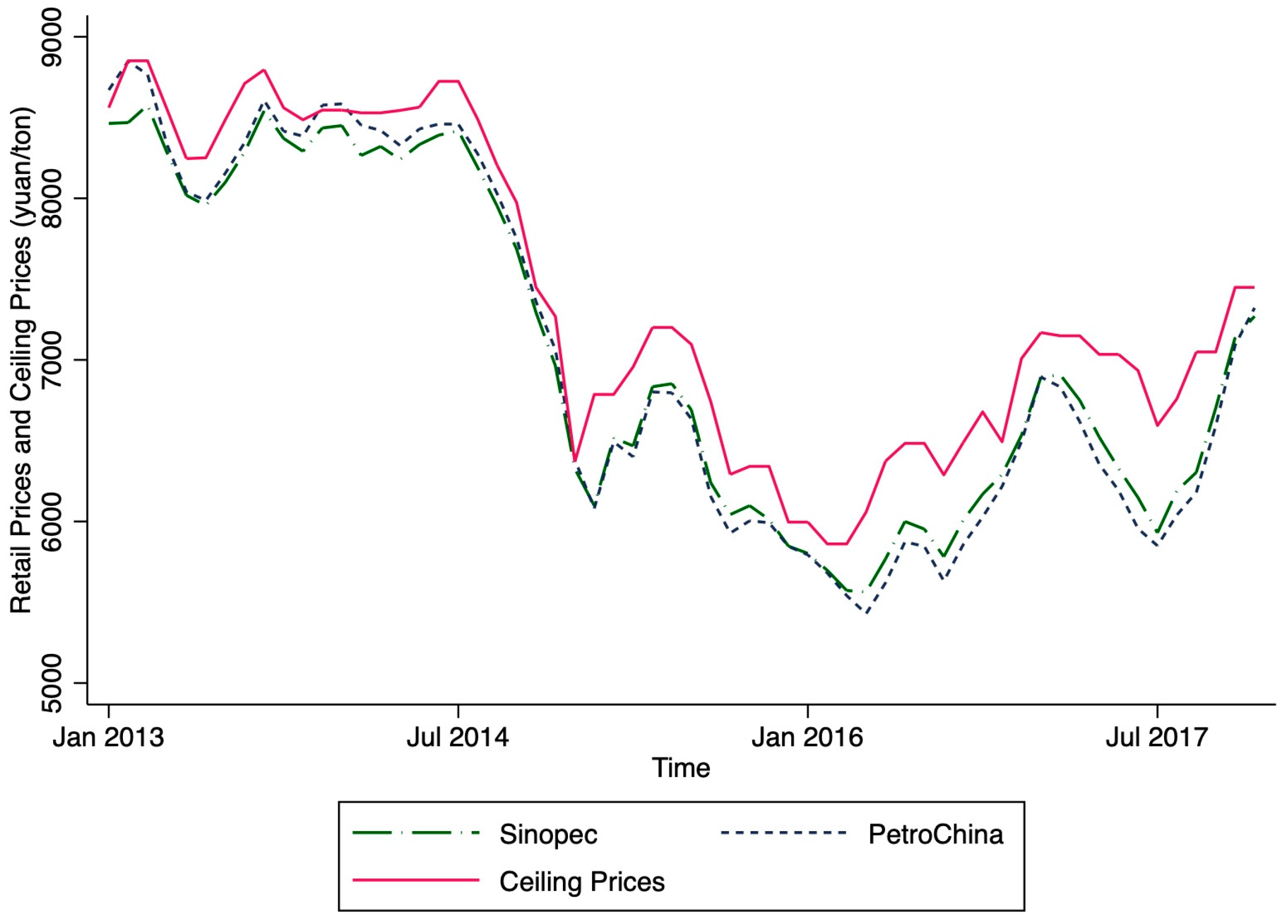Figure 1 intuitively shows the fluctuation of the retail prices of two firms, which exhibits a nearly identical pattern. The two lines are almost perfectly overlapping throughout the 2013–2017 period. Price adjustments occur simultaneously and in the same magnitude for both firms. This visual evidence points towards strong price coordination or a “follow-the-leader” pricing mechanism, providing preliminary support for the high conjectural variation found in our estimation.

In contrast to the uniformity in pricing, the market scale of the two firms shows significant divergence. Sinopec operates at a substantially larger scale, with mean monthly retail sales of 145,780.4 tons, which is approximately 55.3% higher than PetroChina’s average of 93,865.1 tons. The disparity is even more pronounced at the upper end of the distribution, with Sinopec’s maximum monthly sales reaching 690,000 tons, more than double the maximum recorded for PetroChina (335,694.6 tons).

The cost-side indicators, proxied by wholesale prices, follow a similar pattern of convergence. PetroChina’s mean wholesale price (6322.4 yuan/ton) and Sinopec’s (6370.2 yuan/ton) are closely aligned, reflecting the common international and domestic crude oil price pressures they both face.

The government-mandated ceiling price remains at an average of 7390.8 yuan per ton, with a minimum of 5670 yuan per ton and a maximum of 9280 yuan per ton. On average, the retail prices for both companies consistently remain below the ceiling price, confirming that the policy ceiling serves as a non-binding but influential upper limit for retail competition. The lower standard deviation of the ceiling price (956.9) compared to retail and wholesale prices indicates that administrative price adjustments are relatively more stable than market-driven price movements. This gap between the ceiling and retail prices confirms the existence of a competitive margin, albeit one that is heavily influenced by the policy environment.

In addition to the main pricing variables, the regressions also control for provincial per capita disposable income to account for regional differences in consumers’ purchasing power and underlying diesel demand. This variable is constructed at the quarterly frequency, and its mean, minimum, and maximum values are 15,159.3 yuan, 1683.2 yuan, and 58,988 yuan, respectively, reflecting substantial economic heterogeneity across provinces and over time. The disposable income per capita for each province is obtained from the provinces’ statistical yearbooks.

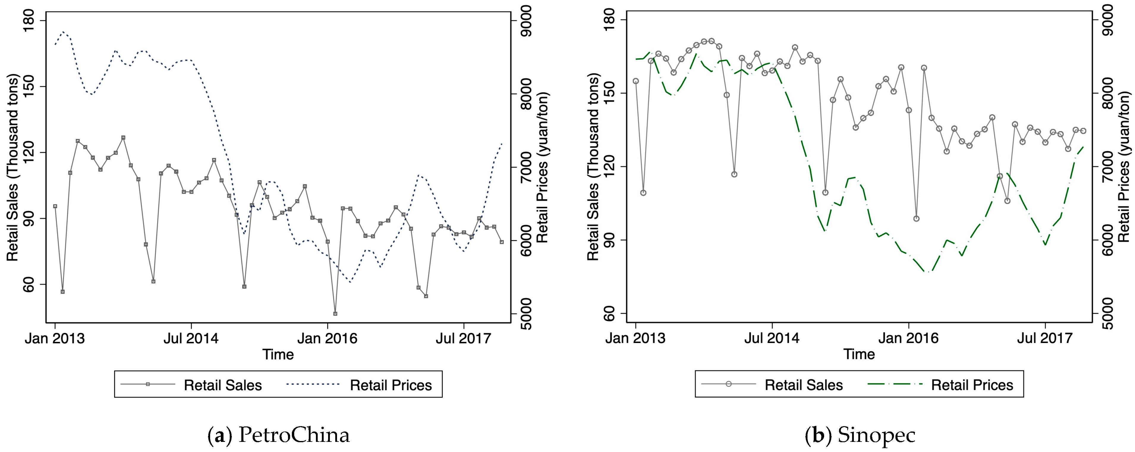
Figure 2 plots the monthly evolution of retail diesel sales and retail prices for PetroChina (panel (a)) and Sinopec (panel (b)) from 2013 to 2017. While the price trends are nearly identical, the sales volume patterns exhibit distinct characteristics. Consistent with the descriptive statistics, Sinopec (Panel b) maintains a consistently higher baseline of retail sales (concentrated in the 120–180 thousand tons range) compared to PetroChina (Panel a, 60–120 thousand tons range). Additionally, both firms show significant seasonal fluctuations in sales, with recurring dips and peaks that likely correspond to the cyclical demand from the agricultural and industrial sectors in different provinces. Third, for both firms, there is a discernible inverse correlation between retail prices and sales volumes. Notably, during the period from late 2014 to early 2016, when retail diesel prices experienced a significant downward trend (consistent with the global decline in crude oil prices, Baumeister & Kilian, 2016), sales volumes for both companies exhibited relatively higher volatility and periodic peaks.

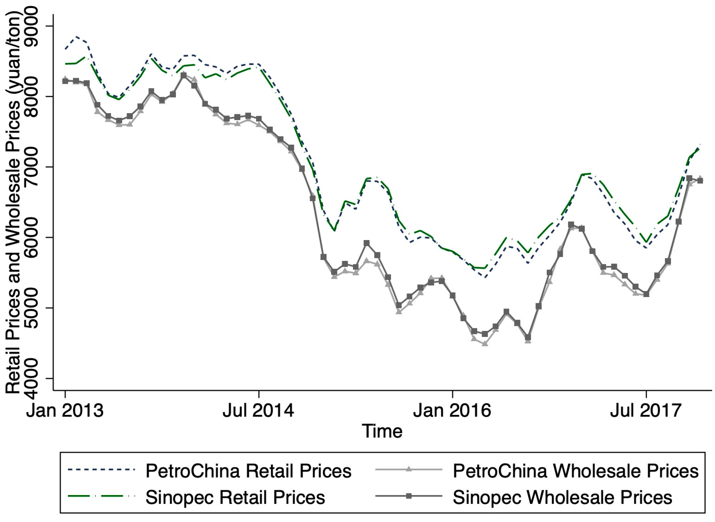
Figure 3 illustrates the relationship between retail and wholesale diesel prices for the two major firms. The wholesale prices of PetroChina and Sinopec almost completely overlap throughout the sample period, with PetroChina’s wholesale price being slightly lower at certain points—mirroring the same pattern observed in their retail prices. This close alignment indicates that both firms adjust retail and wholesale prices in a highly synchronized manner, with only minor and consistent differences between them. The symmetry assumption maintained in the model concerns the key behavioral parameters governing firms’ strategic responses, rather than equality in market size or sales volume. In this sense, symmetry is imposed as a tractable benchmark for identifying the conduct index, following the logic of Karp and Perloff (1989).2

4.3. Estimation of Demand and Price Adjustment Equations

The descriptive patterns above suggest a high degree of price synchronization between the two firms. However, they should be viewed as descriptive evidence only, which motivates the structural analysis.

At the same time, the descriptive evidence is informative about how the model maps into observable market behavior. The close dependence of current prices on their own recent levels is consistent with a relatively high degree of own-price persistence, as captured by $G_1$. The near-synchronous movement of the two firms’ prices suggests that each firm responds closely to the rival’s previous pricing decisions, which is the type of strategic interdependence summarized by $G_2$. The fact that retail prices remain tightly clustered and evolve gradually around an administratively salient ceiling is also consistent with the idea that pricing adjustment is subject to frictions and focal constraints rather than being fully flexible in every period. For this reason, the structural model is useful precisely because it separates descriptive price alignment from the deeper question of whether such alignment reflects dynamic adjustment, institutional focal points, or stronger conduct.

As modelled in Section 2 and Section 3, PetroChina and Sinopec engage in a dynamic game of price competition. To proceed with our analysis and identify the variable of interest $\nu$, we would need to know the values of parameters in the demand function, i.e., ($\theta ,\eta$) in Equation (1), as well as the values of parameters in the price adjustment equation, ($G_1$,$G_2$) in Equation (8).

The demand equations are estimated using the three-stage least squares (3SLS) estimation method, where we control for the effect of per capita income, time trend terms (a time trend, time squared, and time cubed), and province-by-year fixed effects. The instruments for retail prices include the wholesale prices of the two firms and the government-imposed ceiling price. Constraints on the coefficients are imposed during the estimation to represent the symmetry of players, i.e., ${\theta }_1={\theta }_2,{\eta }_1={\eta }_2$. The first-stage results reported in

Table A2. First-stage regressions for endogenous retail prices.

	Endogenous Variables
Variables	PetroChina Retail Prices	Sinopec Retail Prices
PetroChina Wholesale Prices	0.243 ***	0.079 ***
	(0.026)	(0.023)
Sinopec Wholesale Prices	0.141 ***	0.239 ***
	(0.031)	(0.027)
Ceiling Prices	0.653 *** (0.024)	0.690 *** (0.021)
Control Variables	Yes	Yes
Province-by-Year FE	Yes	Yes
Time Trend	Yes	Yes
Time Squared	Yes	Yes
Time cubed	Yes	Yes
N	1591	1591
R2	0.962	0.968
F-statistics	798.38	986.85
Sargan Statistic	37.633 ***	6.819 **

Notes: This table reports the first-stage regressions for the endogenous retail price variables in the demand system. The dependent variables are PetroChina retail prices and Sinopec retail prices, respectively. The excluded instruments are PetroChina wholesale prices, Sinopec wholesale prices, and the government ceiling price. All specifications additionally include the full set of control variables, province-by-year fixed effects, and cubic time trends. Standard errors are reported in parentheses. Reported F-statistics are Cragg–Donald Wald tests of the joint significance of the excluded instruments in each first-stage regression. The large first-stage F-statistics (798.38 for PetroChina retail prices and 986.85 for Sinopec retail prices) indicate that the excluded instruments have strong predictive power for the endogenous retail price variables, suggesting that weak-instrument concerns are unlikely to be severe in our setting. The exogeneity of the instruments is justified on economic and institutional grounds discussed in the main text rather than claimed to be directly testable from the first stage alone. *** and ** denote significance at the 1% and 5% levels, respectively.

support the relevance of these instruments, while the exclusion restriction is justified on the economic and institutional grounds discussed above. The estimated demand equations are

$$Q_{it}={\alpha }_{it}-{\theta }_i{p}_{it}+{\eta }_i{p}_{jt}+\gamma X+{\lambda }_{ct}+\tau +\epsilon$$

where ${\lambda }_{ct}$ refers to the province-by-year fixed effect and $\tau$ is time trend term (including a time trend, time squared, and time cubed). $Q_{it}$ refers to the monthly sales of firm i at time t. $p_{it}$ refers to retail prices of firm i at time t. $p_{jt}$ refers to the retail prices of firm j at time t. $X$ is the control variable, Income.

The estimation result can be found in

Table 2. The estimated parameters of demand function.

	Dependent Variables: Sales
Variables	PetroChina	Sinopec
PetroChina Retail Prices	−38.40 ***	35.05 ***
	(8.814)	(8.941)
Sinopec Retail Prices	35.05 ***	−38.40 ***
	(8.941)	(8.814)
Control Variables	Yes	Yes
Province-by-Year FE	Yes	Yes
Time Trend	Yes	Yes
Time Squared	Yes	Yes
Time cubed	Yes	Yes
N †	1591	1591
R2	0.900	0.941

Notes: The table reports the estimations for the parameters in demand function based on the three-stage least squares (3SLS) estimation method. The dependent variables are the monthly sales of diesel of Sinopec and PetroChina. The instruments for retail prices include wholesale prices of the two firms and the price ceilings set by the government. The estimation sample includes 1591 observation. Constraints on the coefficients are imposed during the estimation to represent the symmetry of players. The standard errors are in parentheses. *** denote significance at the 1% levels. ^† The smaller estimation sample in Table 2 arises because the demand system additionally matches provincial per capita disposable income, which is available at the quarterly frequency and contains some missing values after matching to the monthly panel. In addition, the inclusion of province-by-year fixed effects further reduces the effective estimation sample, so that the final 3SLS demand estimation is based on 1591 observations.

, where the numbers in parentheses are standard errors. The estimation results show that the values of $\theta$ and $\eta$ are 38.40 and 35.05, respectively, and both are statistically significant at the 1% level.

The ($G_1$,$G_2$) in the price adjustment Equation (8) is estimated using the seemingly unrelated equation method. Each company’s price is regressed on the lagged prices of both companies, where we also control the time trend terms (a time trend, time squared, and time cubed) and province-by-year fixed effects. The results can be found in

Table 3. The estimated parameters in price adjustment equation.

	Dependent Variables: Retail Prices
Variables	PetroChina	Sinopec
First Lag Price of PetroChina.	0.567 ***	0.182 ***
	(0.015)	(0.014)
First Lag Price of Sinopec.	0.182 ***	0.567 ***
	(0.014)	(0.015)
Province-by-Year FE	Yes	Yes
Time Trend	Yes	Yes
Time Squared	Yes	Yes
Time cubed	Yes	Yes
N †	1729	1729
R2	0.917	0.945

Notes: The table reports the estimations for the parameters in price adjustment equation based on the seemingly unrelated equation method. The dependent variables are the monthly retail prices of Sinopec and PetroChina. Standard errors are reported in parentheses. The estimation sample includes 1729 observations. Constraints on the coefficients are imposed during the estimation to represent the symmetry of players. The standard errors are in parentheses. *** denote significance at the 1% levels. ^† The sample size in Table 3 is smaller than 1860 because the price-adjustment equations require lagged retail prices and include province-by-year fixed effects. As a result, observations are lost mainly because the lag structure removes the first available month in each province-specific series and because the fixed-effects specification excludes cells without sufficient within-group variation, leaving 1729 observations for the SUR estimation.

. The estimated coefficients of $G_1$ and $G_2$ are 0.57 and 0.18, respectively, both of which are statistically significant at 1% level.

4.4. Calculating the Market Competitiveness Measure

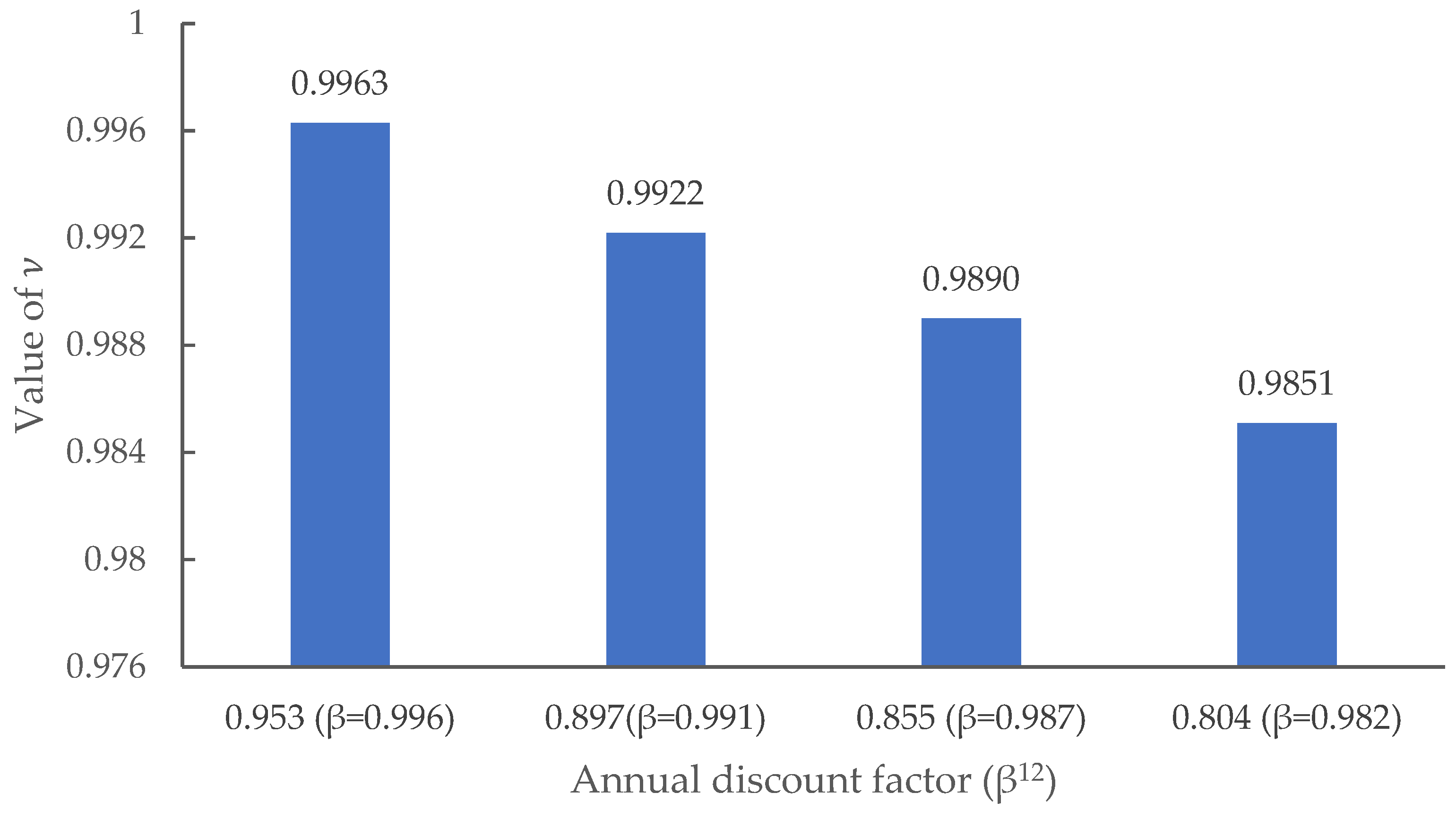
After the empirical estimation of the demand function and price-adjustment equation in Section 4.3, we can now calculate the market competitiveness measure $\nu$ Plugging the estimated values of $\theta$, $\eta$, $G_1$, and $G_2$ into the system of Equations (9a)–(9e), and choosing a monthly discount factor of 0.996 (equivalent to an annual discount factor of 0.95), we solve for the unknown structural parameters. We obtain a standard error of 0.249 for $\nu$ by the Delta method, and thus reject the null hypothesis that the Chinese retail oil market is perfectly competitive ($\nu$ = −1) or characterized by independent oligopolistic pricing ($\nu$ = 0).

However, we cannot reject the hypothesis that $\nu =1$ at the 5% level. This indicates that the estimated conduct index is consistent with a highly coordinated or collusion-like outcome under the maintained structure, which complements the descriptive evidence of strong price synchronization between the two firms. In the institutional setting of China’s retail oil market, regulation and government price ceilings may serve as mechanisms that facilitate and sustain this alignment in pricing behavior. Accordingly, our findings suggest that market outcomes in this regulated environment are more consistent with conduct close to the collusive benchmark. As shown further in Appendix A.6, this qualitative conclusion remains stable across a reasonable range of alternative discount factors.

Following Karp and Perloff (1989), the point of the model is to locate observed behavior relative to benchmark regimes inside a fully specified dynamic framework. This logic is similar to other conduct parameter and market power studies, where the estimated conduct measure is informative only under the maintained assumptions about demand, strategic interaction, and market structure (Bresnahan, 1982; Lau, 1982; Nevo, 2001; Wolfram, 1999; Puller, 2007). Accordingly, our estimate should be read as evidence consistent with a highly coordinated or collusion-like outcome under the maintained structure, rather than as direct proof of explicit collusion. This distinction is especially important in retail oil markets, where price alignment may also arise from focal-point regulation, price leadership, or repeated interaction even in the absence of direct communication (Byrne & de Roos, 2019; Clark & Houde, 2013; Zhang et al., 2020).

5. Concluding Remarks

This paper extends the dynamic oligopoly framework of Karp and Perloff (1989) to a price-setting environment with differentiated goods and explicit price stickiness, and applies that framework to the Chinese retail oil market. Within this dynamic structure, we use an index analogous to price conjectural variation to evaluate market competitiveness. The empirical results show that the estimated conduct parameter is closer to the collusive benchmark than to the competitive or independent-pricing benchmarks within the maintained model. Taken together with the descriptive evidence of strong price synchronization, this suggests that pricing outcomes in the Chinese retail oil market are consistent with a highly coordinated or collusion-like outcome under the maintained structure.

More broadly, the paper contributes to the conduct literature by showing that market competitiveness in posted-price industries cannot be inferred from price synchronization alone. Descriptive indicators such as price uniformity, synchronized timing, or proximity to a regulatory ceiling are useful warning signals, but they do not by themselves map observed pricing outcomes into a structural benchmark of firm conduct (Eckert & West, 2005; Zhang et al., 2020). Similar prices may reflect common cost shocks, institutional focal points, regulated adjustment rules, or lagged strategic responses, rather than a purely static notion of market power. By embedding the conduct parameter in a dynamic price-setting model, this paper provides a structural way to distinguish simple price co-movement from stronger strategic internalization among firms.

The proposed conduct index also complements traditional static conduct and markup approaches. Static models have provided important tools for identifying market power and competitive behavior (Bresnahan, 1982; Lau, 1982; Nevo, 2001), but they typically abstract from lagged price adjustment and dynamic state dependence. This limitation is especially relevant in markets where firms post prices repeatedly, observe rivals’ past prices, and adjust with delay rather than instantaneously. In such settings, a static margin may confound market power with price persistence. Our dynamic framework adds information precisely because it requires the researcher to account for both current strategic interaction and lagged adjustment behavior. The index should therefore be interpreted as a quantitative screening and monitoring tool, rather than as a legal test of collusion.

For the Chinese retail oil market, the index has practical relevance for regulatory monitoring. It can help regulators evaluate whether parallel price movements primarily reflect common cost changes, regulatory price ceilings, dynamic adjustment frictions, or stronger strategic internalization by the dominant firms. The index may also be useful for comparing market conduct before and after reforms to the ceiling price regime. For example, if observed prices remain tightly clustered near the coordination benchmark even after changes in institutional conditions, this would be more concerning than descriptive evidence of parallel price movements alone. The findings therefore highlight an important policy trade-off: while retail price ceilings may protect consumers from extreme price spikes, they may also create salient focal points that reduce incentives for independent undercutting and facilitate sustained price alignment among dominant firms.

The framework may also be adapted to other price-setting industries with similar institutional features. Electricity markets, for example, often involve repeated pricing or offer behavior, transparent market conditions, regulatory constraints, and gradual adjustment. Existing studies show that market power assessment in electricity markets is particularly challenging when repeated interaction, regulation, and contractual structures jointly shape observed prices (Wolfram, 1999; Puller, 2007; Bushnell et al., 2008). Although our model is not intended to be applied mechanically to all regulated energy markets, it is especially informative in environments characterized by high price transparency, repeated interaction, sticky or regulated price adjustment, and sufficiently rich panel data on prices and demand.

At the same time, the interpretation of the empirical results remains conditional on the maintained assumptions of the model, including the symmetry assumption, the linear-quadratic structure, and the assumed discount factor. Future research could extend the framework to allow for firm asymmetries, multi-product competition, heterogeneous adjustment costs, or richer regulatory constraints. Such extensions would further broaden the empirical relevance of dynamic conduct measures in concentrated and regulated posted-price markets.