On Collusion Sustainability and the Elasticity of Substitution

Abstract

We analyze the relationship between collusion sustainability in an infinitely repeated game using trigger strategies and the elasticity of substitution. To this end, we adopt a demand function with constant elasticity of substitution between the differentiated goods. Since our model exhibits a one-to-one relationship between the elasticity of substitution and demand price elasticity, we demonstrate that a larger elasticity decreases the sustainability of collusion. Intuitively, a more elastic demand function causes the increase in deviation profits to compensate for the increase in collusive profits, making collusion less easily sustained. This result holds regardless of whether firms compete in quantities or prices.

1. Introduction

Studying the factors that facilitate collusive practices is a major concern for antitrust authorities, as these practices allow firms to exert market power and artificially restrict competition. A very well-known threat to competition arises when several firms engage in what economists refer to as tacit collusion.1 Tacit collusion typically arises when firms interact repeatedly. Following Friedman’s (1971) approach and subsequent contributors, we know that firms can maintain collusive agreements by using the threat of reversion to comprehensive non-cooperation if a deviation occurs. The punishment strategy that underpins this result involves firms weighing the short-term gains from deviation against the subsequent losses arising from punishment. If the latter exceeds the former, deviation is deterred. Therefore, collusion is sustainable if and only if firms place sufficient weight on future profits—that is, if their discount factor is not too small. The theoretical literature on this issue is extensive, obtaining a series of standard results on the effects of factors such as transparent prices, frequent interaction, absence of barriers, buyer power, number of firms, and cost asymmetries on the minimum discount factor required for tacit collusion (see Ivaldi et al., 2003 for a summary). Other papers have focused on factors related to the demand side of the market. For instance, Rotemberg and Saloner (1986) show that a positive demand shock hinders collusion by increasing the incentives to deviate and conquer the entire market. Haltiwanger and Harrington (1991) demonstrate that collusion is more easily sustainable if demand growth is prolonged because the incentives to start a price war decrease as collusive profits increase over time. Throughout this literature, the standard assumption has been linear demand, which ignores the effect of the price elasticity of demand on the sustainability of collusion. To the best of our knowledge, the few exceptions include Collie (2004), who uses numerical simulations to find that a larger elasticity of demand makes it easier to sustain collusion at the monopoly price, and subsequently Gallice (2010), who, with discrete prices, and homogeneous Bertrand competition, confirms the results of Collie.

However, most of the empirical literature suggests a negative relationship between price elasticity and collusion likelihood. The intuition is that the gains from fixing higher prices are greater when market demand is more inelastic, because the necessary contraction in output to achieve the higher collusive price is less, and profits are correspondingly higher. Among the copious evidence supporting this point, Levenstein and Suslow (2006) show that cartels can raise prices substantially only if demand is sufficiently inelastic. Their paper reports several case studies of cartels in industries in Europe and the USA—such as Bromine, Cement, Diamonds, Oil, Steel, and Sugar—for which demand was highly inelastic.

To reconcile the (scarce) theoretical results with the empirical evidence, and contrary to Collie (2004) and Gallice (2010), we address this issue by developing a multi-period oligopoly model where firms produce differentiated goods and face a demand function with a constant elasticity of substitution between the differentiated goods. We use subgame perfect Nash equilibrium—henceforth, SPNE—as a solution concept and adopt the particular criterion of restricting strategies to grim trigger strategies. Unfortunately, this demand function generally does not allow explicit analytical solutions to be obtained for the asymmetric allocation that arises when a firm deviates from a collusive agreement.2 However, since our model exhibits a one-to-one relationship between the elasticity of substitution and the demand price elasticity, we can still assess the effect of demand price elasticity on the sustainability of collusion by resorting to numerical and graphical solutions. We find unambiguously that a larger elasticity of substitution decreases the sustainability of collusion. Intuitively, with a more elastic demand function, the increase in the deviation profits compensates for the increase in the collusive profits. As a consequence, collusion sustainability becomes less likely.

Our results thus differ from those of Gallice (2010), whose paper, featuring homogeneous products and Bertrand competition, shows a deviating firm conquers the market regardless of the elasticity of demand. On the other hand, Collie (2004), also with homogeneous products, finds that the larger the elasticity of demand, the lower the price-cost margin when firms collude at the monopoly price. Consequently, deviation profits are undermined because a deviating firm must set a price even closer to marginal costs, thus exploiting an even lower margin. In contrast, we show that with differentiated products, the rise in deviation profits offsets the rise in collusive profits.

2. Quantity Competition

We consider an industry with two firms, each producing a quantity of a differentiated product at a constant marginal cost $c>0$, and a representative consumer with utility U given by

$$U\left(q\right)={\left(\sum _{i=1}^2{q}_i^{\beta }\right)}^{\theta },$$

where q denotes the vector of quantities produced by firms and $q_i$, $i=1,2$, denotes the output produced by firm i.3 The function U is assumed to be homogeneous of degree $\beta \theta$ where (strict) concavity is imposed by restricting $0<\beta \theta <1$. A constant elasticity of substitution $\sigma$ between the differentiated goods is obtained where $\sigma \equiv {\displaystyle \frac{1}{1-\beta }}$. Consequently, a change in $\beta$ is directly associated with a change in $\sigma$ of the same sign. We note that even though price elasticity of demand and the elasticity of substitution are different concepts, with the symmetric formulation used in the present model, the demand price elasticity for variety i is equal to ${\displaystyle \frac{1}{1-\beta }}$. Therefore, our analysis focusing on the effect of $\beta$ is directly applicable to the elasticity of substitution and to the price elasticity.4 Goods are substitutes, independent, or complements if $\beta$ is larger, equal or smaller than 0, respectively, and $\beta =1$ implies homogeneous goods. The inverse demands for firms $i,j=1,2,$ and $i\ne j$ are easily obtained:

$$P_i\left(q\right)=\beta \theta {\left(q_j^{\beta }\right)}^{\theta -1}{q}_i^{\beta -1}$$

(1)

for any strictly positive vector of quantities q. Demand is downward sloping, ${\displaystyle \frac{\partial P_i}{\partial q_i}}<0$. We restrict our attention to the case where goods are substitutes ($\beta \ge 0$) and ${\displaystyle \frac{\partial P_i}{\partial q_j}}\le 0$, $i\ne j$.

We assume that firms compete repeatedly over an infinite horizon with complete information (i.e., each of the firms observes the whole history of actions) and discount the future using a common discount factor $\delta \in (0,1)$. Time is discrete and dates are denoted by $t=1,2,\dots$. In this framework, a pure strategy for firm i is an infinite sequence of functions ${\left\{S_i^t\right\}}_{t=1}^{\infty }$ with $S_i^t:{\sum }^{t-1}⟶\mathcal{Q}$ where ${\sum }^{t-1}$ is the set of all possible histories of actions (output choices) of all firms up to $t-1$, with typical element ${\varrho }_j^{\tau }$, $j=1,2$, $\tau =1,\dots ,t-1$, and $\mathcal{Q}$ is the set of output choices available to each firm. Following Friedman (1971), we restrict our attention to the case where each firm is only allowed to follow grim trigger strategies. In other words, these strategies require firms to adhere to the collusive agreement until a defection occurs, in which case they revert forever to the static Cournot equilibrium.

Abusing notation, let $q_i^c$ and $q_i^n$ denote the output corresponding, respectively, to collusion and Cournot noncooperative behavior. Since we restrict attention to trigger strategies, ${\left\{S_i^t\right\}}_{t=1}^{\infty }$ can be specified as follows. At $t=1$, $S_i^1=q_i^c$, while at $t=2,3,\dots$

$$S_i^t\left({\varrho }_j^{\tau }\right)=\left\{\begin{array}{c}{q}_i^c\mathrm{if}{\varrho }_j^{\tau }=q_j^c\mathrm{for}\mathrm{all}j=1,2\mathrm{and}\tau =1,\dots ,t-1\\ q_i^n\mathrm{otherwise}\end{array}\right.$$

(2)

For a given value of c, the symmetric static Cournot equilibrium for firm i$=1,2$ can be easily obtained:

$$\begin{array}{c}{q}_i^n(\beta ,\theta )={\left({\displaystyle \frac{c}{{\beta }^2\theta }}\right)}^{{\displaystyle \frac{1}{\beta \theta -1}}}\\ {\Pi }_i^n(\beta ,\theta )=\beta \theta q_i^n{(\beta ,\theta )}^{\beta \theta }-q_i^n(\beta ,\theta )c\end{array}$$

(3)

On the other hand, the collusive quantities and profits in the one-stage game are as follows:

$$\begin{array}{c}{q}_i^c(\beta ,\theta )={\left({\displaystyle \frac{c}{{\left(\beta \theta \right)}^2}}\right)}^{{\displaystyle \frac{1}{\beta \theta -1}}}\\ {\Pi }_i^c(\beta ,\theta )=\beta \theta {\left(q_i^c(\beta ,\theta )\right)}^{\beta \theta }-q_i^c(\beta ,\theta )c\end{array}$$

(4)

Finally, if firm i optimally deviates from the collusive outputs expressed in (4), individual profits are maximized assuming that the other firm still produces according to (4). Deviation outputs and profits can also be easily obtained:

$$\begin{array}{c}{q}_i^d(\beta ,\theta )={\left({\displaystyle \frac{{\xi }^{\beta -\beta \theta }c}{{\beta }^2\theta }}\right)}^{{\displaystyle \frac{1}{\beta -1}}}\\ {\Pi }_i^d(\beta ,\theta )=(q_i^d{(\beta ,\theta ))}^{\beta }\theta \beta {\xi }^{\beta (\theta -1)}-q_i^d(\beta ,\theta )c\end{array}$$

(5)

where $\xi \equiv {\displaystyle \frac{c}{{\left(\beta \theta \right)}^2}}$. Firms producing $q_i^c(\beta ,\theta )$ in each period can be sustained as a SPNE of the repeated game if and only if the following conditions are satisfied:

$${\Pi }_i^c(\beta ,\theta )\ge {\Pi }_i^d(\beta ,\theta )-\delta ({\Pi }_i^d(\beta ,\theta )-{\Pi }_i^n(\beta ,\theta ))\mathrm{for}i=1,2.$$

(6)

Then, since we assume that firms compete repeatedly over an infinite horizon, it is well known that there is a multiplicity of possible SPNE of this repeated game because condition (6) can be satisfied for different collusive outputs. To select among such equilibria, we follow the standard approach in the literature and, thereby, we choose the symmetric profit maximizing allocation for the colluding firms.5 Then, if $\delta$ exceeds a certain critical level, (6) is not a binding constraint, and the distribution of output is the symmetric distribution of the output of a unique firm. If $\delta$ is below that critical level, (6) is a binding constraint. In this case, we consider that collusion is not sustainable. Therefore, we focus on the equilibrium characterized in (4). In other words, if $\delta$ exceeds a certain critical level, the inequalities described in (6) are satisfied. We denote this critical value of the discount factor by $\tilde{\delta }(\beta ,\theta )$ where $q_i^c(\beta ,\theta )$ is a SPNE of the repeated game if $\delta \ge \tilde{\delta }(\beta ,\theta )$. Rearranging (6), we obtain that $\delta \ge \tilde{\delta }(\beta ,\theta )\equiv {\displaystyle \frac{{\Pi }_i^d(\beta ,\theta )-{\Pi }_i^c(\beta ,\theta )}{{\Pi }_i^d(\beta ,\theta )-{\Pi }_i^n(\beta ,\theta )}}\equiv (1-{\displaystyle \frac{{\Pi }_i^c(\beta ,\theta )}{{\Pi }_i^d(\beta ,\theta )}})/(1-{\displaystyle \frac{{\Pi }_i^n(\beta ,\theta )}{{\Pi }_i^c(\beta ,\theta )}})$ The marginal cost of the firms can be normalized to unity, $c=1$, without any loss of generality since the profit ratios: ${\displaystyle \frac{{\Pi }_i^n(\beta ,\theta )}{{\Pi }_i^c(\beta ,\theta )}}$, and ${\displaystyle \frac{{\Pi }_i^c(\beta ,\theta )}{{\Pi }_i^d(\beta ,\theta )}}$ are independent of c so that the critical discount factor $\tilde{\delta }(\beta ,\theta )$ will also be independent of the marginal cost of production.6 We can also note that $0<\tilde{\delta }(\beta ,\theta )<1$ is true as long as the Prisioner’s Dilemma scheme is satisfied, namely, when ${\Pi }_i^d(\beta ,\theta )>{\Pi }_i^c(\beta ,\theta )>{\Pi }_i^n(\beta ,\theta )$. On the other hand, $\theta$ basically captures the degree of convexity of the demand function, and since, as mentioned in the introduction, we focus on the effect of $\beta$ (due to its direct relationship with $\sigma$) on collusion sustainability, we assign a particular value to $\theta$. Let us assume for simplicity that $\theta =1/3$. We are now ready to present our first result (

Table 1. Numerical simulations that corroborate Result 1.

$\mathit{\beta }$	$\tilde{\mathit{\delta }}(\mathit{\beta },\frac{1}{10})$	$\mathit{\beta }$	$\tilde{\mathit{\delta }}(\mathit{\beta },\frac{3}{10})$	$\mathit{\beta }$	$\tilde{\mathit{\delta }}(\mathit{\beta },\frac{3}{5})$	$\mathit{\beta }$	$\tilde{\mathit{\delta }}(\mathit{\beta },\frac{7}{10})$	$\tilde{\mathit{\delta }}(\mathit{\beta },\frac{4}{5})$
0.1	0.715	0.1	0.621	0.1	0.555	0.1	0.537	0.523
0.2	0.758	0.2	0.649	0.2	0.566	0.2	0.546	0.528
0.3	0.806	0.3	0.684	0.3	0.581	0.3	0.557	0.535
0.5	0.913	0.5	0.779	0.5	0.632	0.5	0.593	0.558
0.6	0.961	0.6	0.884	0.6	0.674	0.6	0.624	0.578
0.7	0.991	0.7	0.917	0.7	0.737	0.7	0.673	0.610
0.8	0.999	0.8	0.981	0.8	0.837	0.8	0.759	0.672

). 7

Result 1. 

When firms compete in quantities, a negative relationship between the price elasticity and collusion sustainability is obtained.

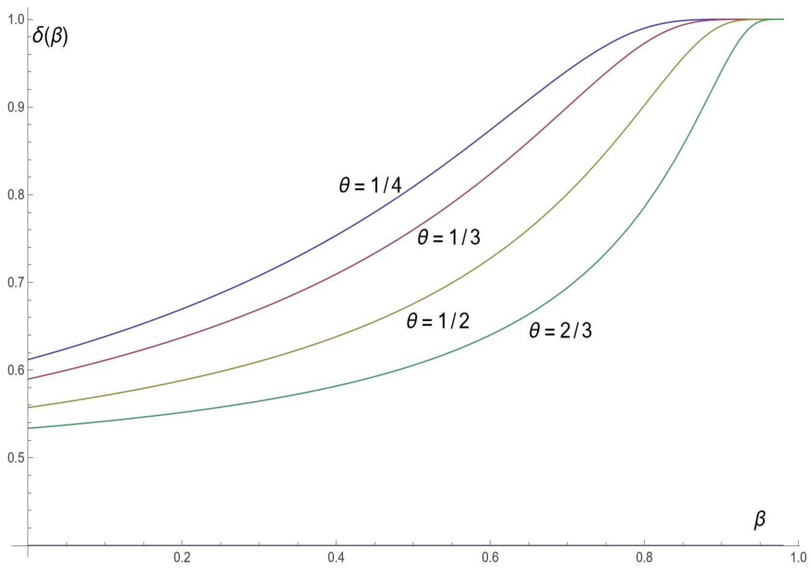
Figure 1 shows that when $c=1$, $\tilde{\delta }(\beta ,\theta )$ increases with $\beta$ for different values of $\theta .$ Consequently, it also increases with $\sigma$.

The intuition is as follows. On one hand, the profit ratio Nash over collusive profits $\left({\displaystyle \frac{{\Pi }_i^n(\beta ,\theta )}{{\Pi }_i^c(\beta ,\theta )}}\right)$ decreases with $\beta$. Consequently, all else being equal, $\tilde{\delta }(\beta ,\theta )$ would decrease with $\beta$ since the punishment is more severe. On the other hand, the profit ratio collusive over deviation profits $\left({\displaystyle \frac{{\Pi }_i^c(\beta ,\theta )}{{\Pi }_i^d(\beta ,\theta )}}\right)$ also decreases with $\beta$, and deviation becomes relatively more profitable with a more elastic demand function. Our result holds because the second effect dominates the first, and collusion becomes less easily sustained as $\beta$ (and thus the elasticity of substitution) increases.8

We provide, as an illustration, a table reporting $\tilde{\delta }(\beta ,\theta )$ (rounded to three decimal places) for different values of $\beta$ and $\theta$ (with $c=1$) to observe that $\tilde{\delta }(\beta ,\theta )$ increases with $\beta$. Further simulations are provided in the Appendix A.

3. Price Competition

We test whether our previous result hinges on the assumption of quantity competition. To this end, we consider the case of price competition in this section. From the system of inverse demand functions described in (1), we can easily obtain the direct demand function for firm $i=1,2$, $i\ne j$:

$$D_i\left(p\right)={\left(\beta \theta \right)}^{{\displaystyle \frac{1}{1-\beta \theta }}}{\displaystyle \frac{p_i^{\frac{1}{\beta -1}}}{{({\sum }_j{p}_j^{\frac{\beta }{\beta -1}})}^{\frac{1-\theta }{1-\theta \beta }}}}$$

(7)

for any strictly positive price vector p. We also note that $1>\theta >0$ and $0<\beta <1$ imply that ${\displaystyle \frac{1-\theta }{1-\theta \beta }}\in (0,1)$. Under these assumptions, it is easy to check that the demand functions are downward sloping and that the goods are substitutes.

For a given value of c, the Nash equilibrium price and profits can be easily obtained:

$$\begin{array}{c}{p}_i^n\left(\beta \right)={\displaystyle \frac{c}{\beta }}\\ {\widehat{\Pi }}_i^n(\beta ,\theta )={({\displaystyle \frac{c}{\beta }})}^{{\displaystyle \frac{1}{\beta \theta -1}}}{\left(\beta \theta \right)}^{{\displaystyle \frac{1}{1-\beta \theta }}}.\end{array}$$

(8)

On the other hand, the collusive prices and profits are as follows:

$$\begin{array}{c}{p}_i^c(\beta ,\theta )={\displaystyle \frac{c}{\beta \theta }}\\ {\widehat{\Pi }}_i^c(\beta ,\theta )={({\displaystyle \frac{c}{\beta \theta }})}^{{\displaystyle \frac{\beta \theta }{\beta \theta -1}}}{\left(\beta \theta \right)}^{{\displaystyle \frac{1}{1-\beta \theta }}}(1-\beta \theta ).\end{array}$$

(9)

Finally, if a firm optimally deviates from the collusive prices expressed in (9), individual profits are maximized assuming that the other firm still sets a price equal to $p_i^c(\beta ,c)$. Deviation profits can also be easily obtained:

$${\widehat{\Pi }}_i^d(\beta ,\theta )=(1-\beta ){({\displaystyle \frac{c}{\beta }})}^{{\displaystyle \frac{\beta }{\beta -1}}}{({\displaystyle \frac{c}{\beta \theta }})}^{{\displaystyle \frac{\beta (1-\theta )}{(\beta -1)(\beta \theta -1)}}}{\left(\beta \theta \right)}^{{\displaystyle \frac{1}{1-\beta \theta }}}.$$

(10)

Before proceeding as in the previous section to obtain the cutoff of the discount factor needed in order for the prices described in (9) to be a SPNE of the repeated game, we should first note that ${\widehat{\Pi }}_i^c(\beta ,\theta )$ is only larger than ${\widehat{\Pi }}_i^n(\beta ,\theta )$ if c is sufficiently large. In other words, collusion only leads to larger profits than those obtained in the Nash equilibrium if firms are sufficiently inefficient. The intuition is that collusion implies raising the price and, consequently, producing a low quantity. However, if c is sufficiently low, firms always obtain a larger profit by decreasing the price to produce at a very low cost. More precisely, we can check that ${\widehat{\Pi }}_i^c(\beta ,\theta )>{\widehat{\Pi }}_i^n(\beta ,\theta )$ if $c>\beta {\theta }^{{\displaystyle \frac{\beta \theta }{\beta \theta -1}}}/(1-\beta \theta )$. In other words, we need to assume that the last inequality is satisfied to obtain a Prisoner’s Dilemma structure where tacit collusion may be profitable. Then, and equivalently to the inequalities described in (6), we can obtain a cutoff of the discount factor, that we denote by $\widehat{\delta }(\beta ,\theta ,c)$, in such a way that $p_i^c(\beta ,\theta )$ is a SPNE of the repeated game if $\delta \ge \widehat{\delta }(\beta ,\theta ,c)$. As in the previous section, we assume for simplicity that $\theta =1/3$. In this case, it is immediate to check that if $c\ge {\displaystyle \frac{3\sqrt{3}}{2}}$, then ${\widehat{\Pi }}_i^c(\beta ,1/3)\ge {\widehat{\Pi }}_i^n(\beta ,1/3)$$\forall \beta \in (0,1).$

The following two figures aim to determine whether our previous result hinges on the assumption of quantity competition (

Table 2. Numerical simulations that corroborate Result 2.

$\mathit{\beta }$	$\widehat{\mathit{\delta }}(\mathit{\beta },\frac{1}{10},\frac{3}{2})$	$\mathit{\beta }$	$\widehat{\mathit{\delta }}(\mathit{\beta },\frac{3}{10},\frac{5}{2})$	$\mathit{\beta }$	$\widehat{\mathit{\delta }}(\mathit{\beta },\frac{3}{5},\frac{9}{2})$	$\mathit{\beta }$	$\widehat{\mathit{\delta }}(\mathit{\beta },\frac{7}{10},8)$
0.1	0.158	0.1	0.060	0.1	0.014	0.1	0.007
0.2	0.345	0.2	0.142	0.2	0.033	0.2	0.017
0.3	0.546	0.3	0.253	0.3	0.064	0.3	0.033
0.5	0.876	0.5	0.575	0.5	0.192	0.5	0.101
0.6	0.961	0.6	0.761	0.6	0.323	0.6	0.176
0.7	0.994	0.7	0.912	0.7	0.535	0.7	0.317
0.8	0.999	0.8	0.988	0.8	0.813	0.8	0.582

).9

Result 2. 

When firms compete in prices and c is sufficiently large, a negative relationship is obtained between the price elasticity and collusion sustainability.

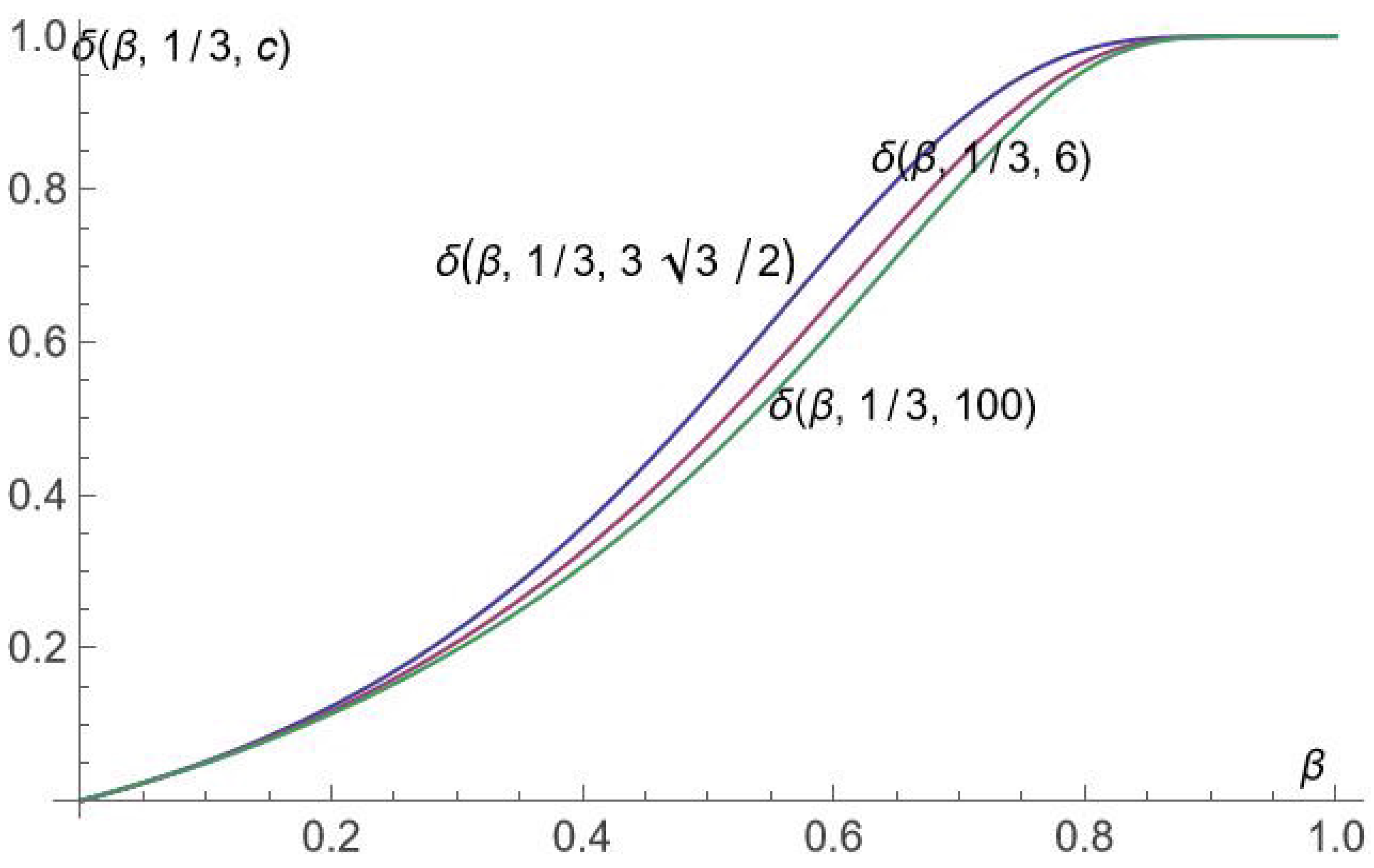
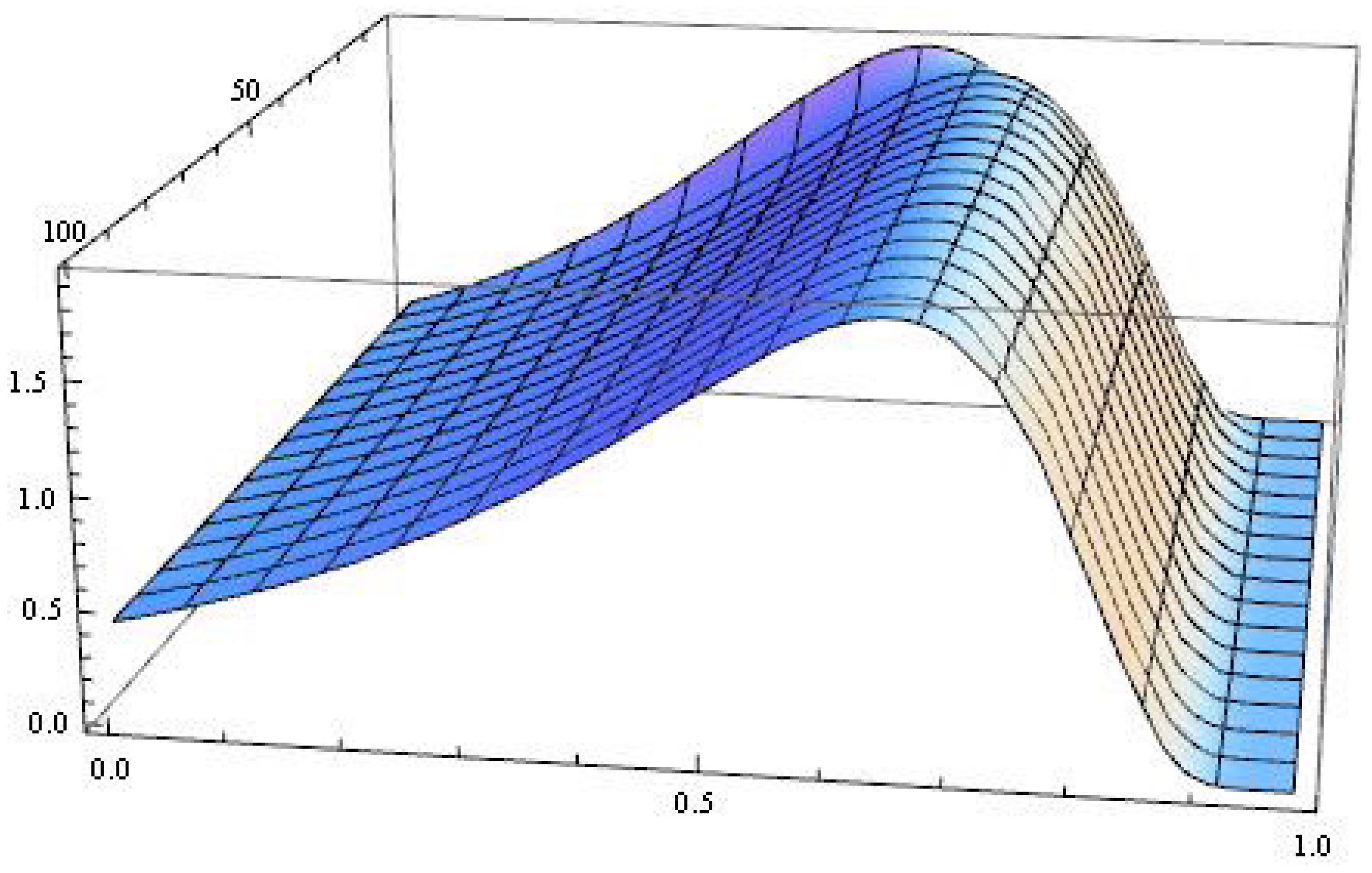
Figure 2 shows that $\widehat{\delta }(\beta ,1/3,c)$ increases with $\beta$ for different values of c ($\sqrt[2]{3}/2,6,$ and 100). Figure 3 shows that the derivative of $\widehat{\delta }(\beta ,1/3,c)$ with respect to $\beta$ is positive for a wide range of values of c (between ${\displaystyle \frac{3\sqrt{3}}{2}}$ and 100). In other words, we have tested the robustness of our result under price competition and established that our result continues to hold.

The intuition parallels the one provided for quantity competition. Namely, if $\beta$ increases, the increase in the deviation profits compensates for the increase in the collusive profits and the decrease in the Nash equilibrium profits.

We provide a table reporting $\widehat{\delta }(\beta ,\theta ,c)$ (rounded to three decimal places) for different values of $\beta$,$\theta$, and c to observe that $\widehat{\delta }(\beta ,\theta ,c)$ increases with $\beta$. Further simulations are also provided in the Appendix A.

4. Concluding Comments

From a theoretical viewpoint, the literature has extensively analyzed the sustainability of collusion in infinitely repeated oligopoly games, relating it to model parameters such as product differentiation, the number of firms, cost asymmetries, or the type of competition (e.g., Bertrand or Cournot). This literature has been mostly restricted to a particular functional form (namely, linear demand), ignoring the effect of the demand function’s elasticity on collusion sustainability. Our results demonstrate a clear, unambiguous effect: a larger price elasticity of substitution reduces the sustainability of collusion. This is important because our model features a one-to-one relationship between the elasticity of substitution and the demand price elasticity.

Admittedly, while a low market elasticity of demand may increase the likelihood of collusion, our message is not that a high market elasticity implies that a high elasticity of market demand implies that collusion cannot exist. The market elasticity we are dealing with in the present work is, to some extent, the pre-collusion elasticity. If, in contrast, we consider the price elasticity when collusive activities have already occurred, then a high elasticity may be consistent with the existence and persistence of collusion because firms have managed to raise prices up to (or near) the monopoly price. That is, a high price elasticity may also coexist with successful collusion. This is an important feature because a high likelihood of collusive behavior among firms severely diminishes consumer welfare and surplus. When competitors tacitly (or explicitly) agree to fix prices or restrict output, the competitive pressure that typically drives prices down toward marginal cost is eliminated. This anti-competitive practice allows the colluding firms to operate closer to a shared monopoly, resulting in supra-competitive prices. Consequently, consumers are forced to pay higher prices, which transfers wealth from consumers to producers, significantly eroding consumer surplus and, thereby decreasing welfare. The limited context of the present model is acknowledged: to analyze real-world cases of collusion, cost asymmetries, firms’ capacities, or more general cost functions should also be considered. An interesting extension would be to examine larger oligopolies. In this context, the tacit collusion literature has shown that the critical threshold for the discount factor (above which collusion is sustainable) increases with the number of firms because, with more firms, each firm receives a smaller share of the collusive gains, and the benefits of cheating grow (see, for example, Vives, 1999). Therefore, one would expect that changing the number of competing firms could generally raise the thresholds reported in our results. Finally, extending this analysis to include harsher punishments—such as the “stick and carrot” strategy from Abreu (1986)—could also be interesting.10 These issues are left for future research.

References

1. Abreu, D. (1986). Extremal equilibria of oligopolistic supergames. Journal of Economic Theory, 39(1), 191–225. [Google Scholar] [CrossRef]
2. Albæk, S., & Lambertini, L. (1998). Collusion in differentiated duopolies revisited. Economics Letters, 59(3), 305–308. [Google Scholar] [CrossRef]
3. Beard, R. (2015). N-firm oligopoly with general iso-elastic demand. Bulletin of Economic Research, 67(4), 336–345. [Google Scholar] [CrossRef]
4. Collie, D. (2004). Collusion and the elasticity of demand. Economics Bulletin, 12(3), 1–6. [Google Scholar]
5. Deneckere, R. (1983). Duopoly supergames with product differentiation. Economics Letters, 11, 37–42. [Google Scholar] [CrossRef]
6. Friedman, J. W. (1971). A non-cooperative equilibrium for supergames. The Review of Economic Studies, 38(1), 1–12. [Google Scholar] [CrossRef]
7. Gallice, A. (2010). The neglected effects of demand characteristics on the sustainability of collusion. Research in Economics, 64(4), 240–246. [Google Scholar] [CrossRef]
8. Haltiwanger, J., & Harrington, J. E., Jr. (1991). The impact of cyclical demand movements on collusive behavior. The RAND Journal of Economics, 22, 89–106. [Google Scholar] [CrossRef]
9. Ivaldi, M., Jullien, B., Rey, P., Seabright, P., & Tirole, J. (2003). The economics of tacit collusion. Final Report for DG Competition, European Commission. Institut d’Économie Industrielle (IDEI). [Google Scholar]
10. Levenstein, M. C., & Suslow, V. Y. (2006). What determines cartel success? Journal of Economic Literature, 44(1), 43–95. [Google Scholar] [CrossRef]
11. Motta, M. (2004). Competition policy: Theory and practice. Cambridge University Press. [Google Scholar]
12. Rotemberg, J. J., & Saloner, G. (1986). A supergame-theoretic model of price wars during booms. The American Economic Review, 76(3), 390–407. [Google Scholar]
13. Vasconcelos, H. (2005). Tacit collusion, cost asymmetries, and mergers. The RAND Journal of Economics, 36, 39–62. [Google Scholar]
14. Vives, X. (1999). Oligopoly pricing: Old ideas and new tools. MIT Press. [Google Scholar]
15. Zhelobodko, E., Kokovin, S., Parenti, M., & Thisse, J. F. (2012). Monopolistic competition: Beyond the constant elasticity of substitution. Econometrica, 80(6), 2765–2784. [Google Scholar] [CrossRef]
Figure 1. Cutoff of the discount factor decreases with the elasticity of substitution under quantity competition.
Games 17 00005 g001
Figure 2. Cutoff of the discount factor decreases with the elasticity of substitution under price competition for a given marginal cost.
Games 17 00005 g002
Figure 3. Cutoff of the discount factor decreases with the elasticity of substitution under price competition for different marginal costs.
Games 17 00005 g003