Weighted Scoring Committees

Abstract

Weighted committees allow shareholders, party leaders, etc. to wield different numbers of votes or voting weights as they decide between multiple candidates by a given social choice method. We consider committees that apply scoring methods such as plurality, Borda, or antiplurality rule. Many different weights induce the same mapping from committee members’ preferences to winning candidates. The numbers of respective weight equivalence classes and hence of structurally distinct plurality committees, Borda commitees, etc. differ widely. There are 6, 51, and 5 plurality, Borda, and antiplurality committees, respectively, if three players choose between three candidates and up to 163 (229) committees for scoring rules in between plurality and Borda (Borda and antiplurality). A key implication is that plurality, Borda, and antiplurality rule are much less sensitive to weight changes than other scoring rules. We illustrate the geometry of weight equivalence classes, with a map of all Borda classes, and identify minimal integer representations.

1. Introduction

Weighted voting games, i.e., simple voting games that allow weighted representations, were first formalized by von Neumann and Morgenstern [1] (Ch. 10). A large body of literature has since investigated the structural properties of collective decisions on binary options. It is, for instance, well known that in a committee with three players, all distributions $\mathbf{w}=(w_1,w_2,w_3)$ of voting weights with $0<w_i<(w_1+w_2+w_3)/2$ for $i\in \{1,2,3\}$ give rise to the same mathematical structure, i.e., the same mapping from voter preferences to decisions under simple majority rule, because any two players can form a winning coalition. Following the tradition of [2,3], various authors have formalized related observations for binary choices by arbitrarily many players, and the literature is still thriving (see, e.g., [4,5]).

Much less is known, however, when committees choose between $m>2$ options. Kurz, Mayer, and Napel ([6], KMN in the following) define “weighted committee games” in order to model decisions on more than two alternatives as concisely as weighted voting games do for binary decisions. For given sets of n voters and $m\ge 2$ candidates, a weighted committee game combines voting weights $\mathbf{w}=(w_1,\dots ,w_n)$ and a baseline social choice rule r to a mapping $r|\mathbf{w}$ from profiles of voter preferences over the candidates to a winning candidate. For a given voting method r, such as plurality rule or pairwise majority voting, KMN investigate equivalence classes of weight distributions: disjoint sets ${\mathit{\epsilon }}_1,\dots ,{\mathit{\epsilon }}_{\xi }$ of voting weights such that $r|\mathbf{w}=r|{\mathbf{w}}^{\prime }\iff \mathbf{w},{\mathbf{w}}^{\prime }\in {\mathit{\epsilon }}_k$, i.e., the collective decision coincides irrespective of the considered preference profile whenever $\mathbf{w}$ and ${\mathbf{w}}^{\prime }$ come from the same class ${\mathit{\epsilon }}_k$, while decisions differ for at least one preference configuration if $\mathbf{w}\in {\mathit{\epsilon }}_k$ and ${\mathbf{w}}^{\prime }\in {\mathit{\epsilon }}_l\ne {\mathit{\epsilon }}_k$.

The respective classes depend on the number m of candidates that the committee decides on, as well as on the baseline decision rule r and the number n of voters. For instance, the weight distributions $\mathbf{w}=(1,1,1)$ and ${\mathbf{w}}^{\prime }=(4,3,2)$ for $n=3$ voters are equivalent in the binary case, where plurality and Borda rule generally coincide with simple majority voting. But $\mathbf{w}$ and ${\mathbf{w}}^{\prime }$ imply different plurality winners for at least some preference configuration for all $m>2$ and then these weights pertain to different classes of plurality committees. Similarly, they belong to different equivalence classes under Borda rule for $m>2$ since $\mathbf{w}$ and ${\mathbf{w}}^{\prime }$ produce different Borda winners for several combinations of committee members’ preferences over three or more candidates.

KMN study only four rules r in detail—three scoring rules (explained below) and one Condorcet rule, which picks the winner of all pairwise votes whenever such a (Condorcet) winner exists. They show that the rules vary widely in the degree to which voting weights make a difference and identify a particularly succinct representative for each equivalence class: integer weights $\overline{\mathbf{w}}$ with minimal ${\parallel ·\parallel }_1$-norm. The objective of this article is to extend the analysis of KMN to the wider family of scoring rules when voters such as shareholders, political parties, etc. decide on three or more alternatives.

A scoring rule r is generally characterized by associating scores $s_1\ge s_2\ge \dots \ge s_m=0$ with the $1\mathrm{st}$, $2\mathrm{nd}$, …, $m\mathrm{th}$ rank in each voter’s individual preference ordering of the candidates. It then selects the candidate who receives the highest total score (up to tie-breaking). For instance, plurality voting on three candidates corresponds to using scores $\mathbf{s}=(s_1,s_2,s_3)=(1,0,0)$, i.e., counting only the number of $1\mathrm{st}$ ranks attributed to each candidate and picking the candidate who is ranked first the most often. The antiplurality rule amounts to $\mathbf{s}=(1,1,0)$: it selects the candidate who receives the fewest last ranks from the voters (or the fewest objections). Under the Borda rule, the score from a given voter for a candidate reflects the number of other candidates that this voter ranks lower. This corresponds to using $\mathbf{s}=(2,1,0)$ or, equivalently, $\mathbf{s}=(1,s,0)$ for $s=\raisebox{1ex}{$1$}\!\left/ \!\raisebox{-1ex}{$2$}\right.$. KMN have focused on these three scoring rules.

After introducing the basic notation (Section 2) and defining equivalence classes of committee games (Section 3), we summarize the algorithmic approach proposed by KMN (Section 4). By applying it, we find that the three scoring rules with $s\in \{0,\raisebox{1ex}{$1$}\!\left/ \!\raisebox{-1ex}{$2$}\right.,1\}$ hold a special position in the family of all scoring rules (Section 5). Numerical computations show that the respective numbers of equivalence classes—6 plurality committees, 51 Borda committees, and 5 antiplurality committees for $n=m=3$—are much smaller than the respective numbers for alternative scoring rules. Rules that are “intermediate” between plurality and Borda (i.e., based on $\mathbf{s}=(1,s,0)$ with $0<s<\raisebox{1ex}{$1$}\!\left/ \!\raisebox{-1ex}{$2$}\right.)$ or between Borda and antiplurality ($\raisebox{1ex}{$1$}\!\left/ \!\raisebox{-1ex}{$2$}\right.<s<1)$ have a more complex geometry and are considerably more sensitive to weight variations than these benchmarks. We show that the weight sensitivity of intermediate scoring rules increases in m without bound (Proposition 4).

Sensitivity to weight changes can matter, e.g., for the incentives to purchase ordinary company shares with voting rights vs. preferred shares without such rights. It also affects the bargaining power of potential party switchers in parliaments and is relevant for international institutions like the International Monetary Fund, which draws on asymmetric voting weights in, e.g., the election of the fund’s Managing Director from up to three shortlisted candidates (see, e.g., [7,8]). The IMF’s “General Review of Quotas” is currently in its 15th round and tries to reform voting weights in response to shifts in global trade flows and finance. It is of political and economic interest whether post-review IMF quotas actually change how member countries’ preferences translate into decisions or if they only make cosmetic changes by moving to a different weight distribution in the same equivalence class.

Decision making is more stable to re-weightings if rules with few equivalence classes are used. Whether such stability is desirable or not depends on the institutional context and one’s perspective. If, for instance, a change in IMF quotas leaves votes in the Executive Board structurally unchanged, then this might be celebrated as a successful quota review by members whose relative voting weight was nominally reduced. Others whose relative voting weight increased may plausibly take the opposite view.

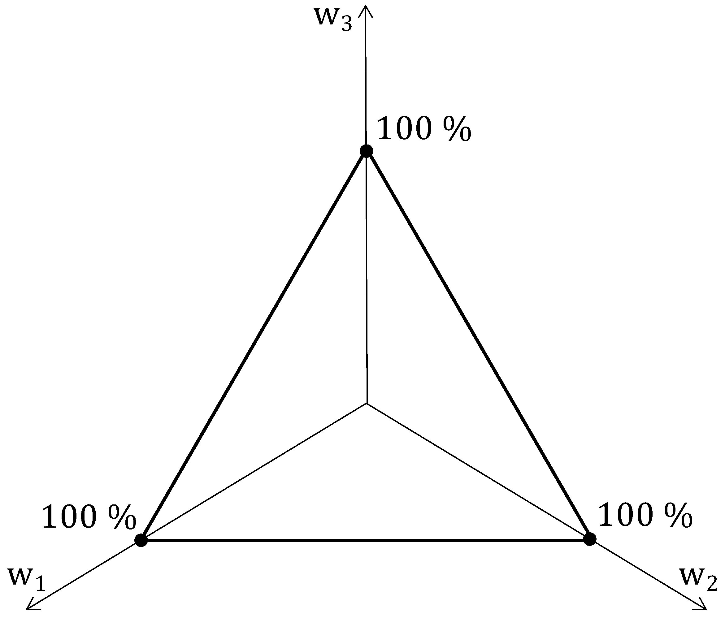
We provide several geometric illustrations of the equivalence classes of different scoring rules for $n=m=3$. They show how attaching greater scores s to voters’ mid-ranked alternatives reduces the scope for a high-weight voter to dominate others. The figures also include a “map” of all 51 Borda equivalence classes. This map allows to easily identify the set of equivalent weights for a given weighted Borda committee. A comprehensive list of minimum integer sum representations of all structurally distinct scoring committees is provided for $n=m=3$ and selected values of $s\in [0,1]$ in Appendix A.

2. Notation and Definitions

2.1. Committees and Scoring Rules

We adopt KMN’s framework and consider finite sets N of $n\ge 2$ players or voters such that each player $i\in N$ has strict preferences $P_i:\{1,\dots ,m\}\to A$ over a set $A=\{a_1,\dots ,a_m\}$ of $m\ge 2$ options or candidates. The set of all $m!$ strict preference orderings on A is denoted by $\mathcal{P}\left(A\right)$. A (resolute) voting rule $\rho :\mathcal{P}{\left(A\right)}^n\to A$ maps each preference profile $\mathbf{P}=(P_1,\dots ,P_n)$ to a single winning alternative $a^{*}=\rho \left(\mathbf{P}\right)$. The combination $(N,A,\rho )$ of a set of voters, a set of alternatives and a particular voting rule, is referred to as a committee (game).

For given N and A, there are $m^{\left(m!{}^n\right)}$ distinct rules $\rho$ and committees. Those which treat all voters $i\in N$ symmetrically are particularly relevant benchmarks: suppose profile ${\mathbf{P}}^{\prime }$ results from applying a permutation $\pi :N\to N$ to profile $\mathbf{P}$, so ${\mathbf{P}}^{\prime }=(P_{\pi \left(1\right)},\dots ,P_{\pi \left(n\right)})$. Then $\rho$ is anonymous if for all such $\mathbf{P}$, ${\mathbf{P}}^{\prime }$ the winning alternative $a^{*}=\rho \left(\mathbf{P}\right)=\rho \left({\mathbf{P}}^{\prime }\right)$ is the same. If we want to emphasize that a considered rule is anonymous, we will write r instead of $\rho$.

We here focus on the family of scoring rules $r^{\mathbf{s}}$ with lexicographic tie-breaking.1 For these, winners are characterized as the lexicographically minimal maximizers of scores. The latter are derived from the positions of the candidates in profile $\mathbf{P}=(P_1,\dots ,P_n)$ and a fixed scoring vector $\mathbf{s}\in {\mathbb{Q}}_{+}^m$. For given $m\ge 2$, this vector $\mathbf{s}=(s_1,s_2,\dots ,s_m)$ consists of rational numbers $s_j$ that satisfy $s_1>s_m=0$ and $s_j\ge s_{j+1}$ for $j\in \{1,\dots ,m-1\}$.

Ballots are tallied by assigning $s_j$ points to any given voter’s j-th ranked candidate. Specifically, let $P_i^{-1}\left(a\right)$ denote the position of alternative $a\in A$ in voter i’s preference ordering $P_i$. Then, voter i’s preferences $P_i$ contribute $s_{P_i^{-1}\left(a\right)}$ to the total score of alternative a. The scoring winner $r^{\mathbf{s}}\left(\mathbf{P}\right)$ at profile $\mathbf{P}$ is the candidate with maximal total score, i.e.,

$$r^{\mathbf{s}}\left(\mathbf{P}\right)\in \underset{a\in A}{arg\; max}\sum _{i\in N}{s}_{P_i^{-1}\left(a\right)}.$$

(1)

If candidates $a_k$ and $a_l$ with $k<l$ have identical scores, the tie is broken in favor of $a_k$. The most prominent scoring rules are plurality rule, which corresponds to $\mathbf{s}=(1,0,\dots ,0)$; antiplurality rule corresponding to $\mathbf{s}=(1,1,\dots ,1,0)$, and Borda rule corresponding to $\mathbf{s}=(m-1,m-2,\dots ,1,0)$.

Scoring rules are particularly appealing social choice rules. Disregarding ties or selecting the entire set of maximizers in Equation (1), they are the only rules that (i) treat all candidates $a\in A$ in a neutral way, (ii) are continuous in the sense that any decision $a^{\ast }$ by a small group of voters will be replaced by a different decision $a^{\ast \ast }$ if a sufficiently large group of voters who would rather choose $a^{\ast \ast }$ joins the electorate, and (iii) have the consistency property that if disjoint groups of voters separately select the same candidate $a^{\ast }$ then their union would also select $a^{\ast }$. See [9].2

For reasons of computational tractability, we will mostly focus on the case of $m=3$ alternatives in what follows. (Re)scaling all scoring vectors $\mathbf{s}=(s_1,s_2,0)$ to vectors ${\mathbf{s}}_s=(1,s,0)$ with $0\le s=\frac{s_2}{s_1}\le 1$ does not affect the score maximizers but conveniently connects plurality rule ($s=0$) and antiplurality rule ($s=1$) such that Borda rule lies halfway in between ($s=\raisebox{1ex}{$1$}\!\left/ \!\raisebox{-1ex}{$2$}\right.$). In particular, letting $s\in [0,1]$ vary captures all possible scoring rules for $m=3$ (see [11]).

2.2. Weighted Scoring Committees

Real-world collective decisions are frequently generated by a non-anonymous voting rule $\rho$. One reason is that the relevant players $i\in N$ may be well-disciplined parties with different seat numbers in a legislature or because stockholders wield as many votes as they own shares. It is then useful to perceive the corresponding rule $\rho$ as the combination of an anonymous baseline voting rule r with non-negative integer voting weights $\mathbf{w}=(w_1,\dots ,w_n)\in {\mathbb{N}}_0^n$ attached to players $1,\dots ,n$. We will adopt the corresponding formalism of KMN.

Letting r denote the family of mappings from preferences to winning alternatives for the considered baseline rule (for all n and m), the weighted voting rule $r|\mathbf{w}$ is defined by

$$r|\mathbf{w}\left(\mathbf{P}\right):=r(\underset{w_1\mathrm{times}}{\underbrace{P_1,\dots ,P_1}},\underset{w_2\mathrm{times}}{\underbrace{P_2,\dots ,P_2}},\dots ,\underset{w_n\mathrm{times}}{\underbrace{P_n,\dots ,P_n}})$$

(2)

for any given anonymous rule r and a non-negative weight vector $\mathbf{w}$ with ${\sum }_{i=1}^n{w}_i>0$.

A committee game $(N,A,\rho )$ is called r-weighted for a given rule r if there exists a weight vector $\mathbf{w}$ such that

$$\rho \left(\mathbf{P}\right)=r|\mathbf{w}\left(\mathbf{P}\right)\mathrm{for}\mathrm{all}\mathbf{P}=(P_1,\dots ,P_n)\in \mathcal{P}{\left(A\right)}^n.$$

(3)

We then refer to $(N,A,r,\mathbf{w})$ as a (weighted) representation of $(N,A,\rho )$ and write the corresponding weighted committee (game) as $(N,A,r|\mathbf{w})$. If the anonymous baseline rule in question is a scoring rule $r^{\mathbf{s}}$, the corresponding game will be called a (weighted) scoring committee. When $m=3$ and the respective scoring vector $\mathbf{s}$ equals ${\mathbf{s}}_s$, we also refer to $(N,A,r^{{\mathbf{s}}_s}|\mathbf{w})$ as an s-scoring committee.

Table 1. Choices from $A=\{a,b,c\}$ for indicated preference profile $\mathbf{P}=(P_1,P_2,P_3)$ when voting weights are $\mathbf{w}=(6,4,3)$ and respective scoring vector ${\mathbf{s}}_s=(1,s,0)$ is in use.

⇒

$r^{{\mathbf{s}}_0}|\mathbf{w}\left(\mathbf{P}\right)=a$    (a has max. plurality score 7) $r^{{\mathbf{s}}_{0.1}}|\mathbf{w}\left(\mathbf{P}\right)=a$  (a has max. score 7) $r^{{\mathbf{s}}_{0.2}}|\mathbf{w}\left(\mathbf{P}\right)=a$  (a has max. score 7) $r^{{\mathbf{s}}_{0.3}}|\mathbf{w}\left(\mathbf{P}\right)=a$  (a has max. score 7) $r^{{\mathbf{s}}_{0.4}}|\mathbf{w}\left(\mathbf{P}\right)=b$  (b has max. score 7.2) $r^{{\mathbf{s}}_{0.5}}|\mathbf{w}\left(\mathbf{P}\right)=b$  (b has max. Borda score 7.5) $r^{{\mathbf{s}}_{0.6}}|\mathbf{w}\left(\mathbf{P}\right)=b$  (b has max. score 7.8) $r^{{\mathbf{s}}_{0.7}}|\mathbf{w}\left(\mathbf{P}\right)=b$  (b has max. score 8.1) $r^{{\mathbf{s}}_{0.8}}|\mathbf{w}\left(\mathbf{P}\right)=b$  (b has max. score 8.4) $r^{{\mathbf{s}}_{0.9}}|\mathbf{w}\left(\mathbf{P}\right)=c$  (c has max. score 9) $r^{{\mathbf{s}}_1}|\mathbf{w}\left(\mathbf{P}\right)=c$    (c has max. antiplurality score 10)

and Figure 1 illustrate that s-scoring committees may indeed induce different mappings from preferences to outcomes for fixed voting weights $\mathbf{w}$ when s is varied. For the indicated preference profile $\mathbf{P}$, the winning candidate crucially depends on the scoring rule in use.

3. Equivalence Classes of Weighted Committees

3.1. Equivalence of Committees

Weighted representations of given committee games are far from unique. Committees $(N,A,r|\mathbf{w})$ and $(N,A,r^{\prime }|{\mathbf{w}}^{\prime })$ are equivalent despite $r\ne r^{\prime }$ or $\mathbf{w}\ne {\mathbf{w}}^{\prime }$ if the respective mappings $r|\mathbf{w}$ and $r^{\prime }|{\mathbf{w}}^{\prime }$ from preference profiles $\mathbf{P}$ to outcomes $a^{\ast }$ coincide, i.e., $r|\mathbf{w}\left(\mathbf{P}\right)=r^{\prime }|{\mathbf{w}}^{\prime }\left(\mathbf{P}\right)$ for all $\mathbf{P}\in \mathcal{P}{\left(A\right)}^n$. Like KMN, we here only consider cases where $r=r^{\prime }$ and focus on structural equivalence. The latter means that two committees $(N,A,r|\mathbf{w})$ and $(N^{\prime },A^{\prime },r|{\mathbf{w}}^{\prime })$ reflect the same decision environment. This can hold even though the labels of players or alternatives differ. Specifically, two r-weighted committee games $(N,A,r|\mathbf{w})$ and $(N^{\prime },A^{\prime },r|{\mathbf{w}}^{\prime })$ are called (structurally) equivalent if

$$\left\{a_j{P}_i{a}_k\iff \tilde{\pi }\left(a_j\right)P_{\pi \left(i\right)}^{\prime }\tilde{\pi }\left(a_k\right)\right\}\Rightarrow \tilde{\pi }\left(r\left|\mathbf{w}\right(\mathbf{P})\right)=r|{\mathbf{w}}^{\prime }\left({\mathbf{P}}^{\prime }\right)$$

(4)

for suitable bijections $\pi :N\to N^{\prime }$ and $\tilde{\pi }:A\to A^{\prime }$.

This definition covers situations where $N=N^{\prime }$ but weights ${\mathbf{w}}^{\prime }$ are a permutation of $\mathbf{w}$. For instance, the plurality or 0-scoring committee $(N,A,r^{{\mathbf{s}}_0}|\mathbf{w})$ obviously has a different attractiveness to player 1 for $\mathbf{w}=(3,2,2)$ than for $(2,3,2)$. Nevertheless, the abstract environment is the same: there is a large player whose most-preferred alternative wins whenever the two smaller players fail to coordinate their votes; otherwise the common favorite of the smaller players wins.

As the number but not the labels of players and alternatives matter, one can write $(r,\mathbf{w}){\sim }_m(r,{\mathbf{w}}^{\prime })$ to denote that r-committee games with m alternatives are structurally equivalent for weight distributions $\mathbf{w}$ and ${\mathbf{w}}^{\prime }$. The relation ${\sim }_m$ and some reference distribution $\overline{\mathbf{w}}\in {\mathbb{N}}_0^n$ with ${\overline{w}}_1\ge {\overline{w}}_2\ge \dots \ge {\overline{w}}_n$ define an equivalence class

$${\mathit{\epsilon }}_{\overline{\mathbf{w}},m}^r:=\left\{\mathbf{w}\in {\mathbb{N}}_0^n|(r,\mathbf{w}){\sim }_m(r,\overline{\mathbf{w}})\right\}.$$

(5)

All weights in a given class ${\mathit{\epsilon }}_{\overline{\mathbf{w}},m}^r$ imply the same distribution of voting power, manipulation incentives, voting paradoxes, strategic voting equilibria, etc. when rule r is invoked to decide on m candidates. KMN show how to explicitly characterize such an equivalence class by linear inequalities.

As there exist at most $m^{\left(m!{}^n\right)}$ distinct committees for given n and m, there are only finitely many disjoint sets ${\mathit{\epsilon }}_{\overline{\mathbf{w}},m}^r$ for any given baseline decision rule r, such as $r^{\mathbf{s}}$. They constitute a finite partition

$$\left\{{\mathit{\epsilon }}_{{\overline{\mathbf{w}}}_{\mathbf{1}},m}^r,{\mathit{\epsilon }}_{{\overline{\mathbf{w}}}_{\mathbf{2}},m}^r,\dots ,{\mathit{\epsilon }}_{{\overline{\mathbf{w}}}_{\xi },m}^r\right\}$$

(6)

of the infinite set ${\mathbb{N}}_0^n$ of weight distributions.

We study this partition for scoring rules and will see below that the number $\xi$ of its elements—and hence the number of structurally distinct weighted committee games for given $r^{\mathbf{s}}$, n, and m—varies widely.

3.2. Relationship between Equivalence Classes for Scoring Rules

Identification and enumeration of structurally distinct weighted scoring committees are running-time-intensive computational tasks. The superexponential growth of $m^{\left(m!{}^n\right)}$ already makes the exploration of committees with a small number of players that decide on few alternatives quite difficult. Before we turn to the details, let us recall three analytical observations by KMN for the most prominent scoring rules (cf. the respective Propositions 3, 4, and 6 and proofs):

Proposition 1.

The plurality partitions $\left\{{\mathit{\epsilon }}_{{\overline{\mathbf{w}}}_{\mathbf{1}},m}^{r^P},\dots ,{\mathit{\epsilon }}_{{\overline{\mathbf{w}}}_{\xi },m}^{r^P}\right\}$ of ${\mathbb{N}}_0^n$ coincide for all $m\ge n$.

Proposition 2.

The antiplurality partitions $\left\{{\mathit{\epsilon }}_{{\overline{\mathbf{w}}}_{\mathbf{1}},m}^{r^A},{\mathit{\epsilon }}_{{\overline{\mathbf{w}}}_{\mathbf{2}},m}^{r^A},\dots ,{\mathit{\epsilon }}_{{\overline{\mathbf{w}}}_{\xi },m}^{r^A}\right\}$ of ${\mathbb{N}}_0^n\setminus \left\{\mathbf{0}\right\}$ consist of $\xi =n$ equivalence classes identified by weight vectors ${\overline{\mathbf{w}}}_{\mathbf{1}}=(1,0,\dots ,0),{\overline{\mathbf{w}}}_{\mathbf{2}}=(1,1,\dots ,0),\dots ,$ ${\overline{\mathbf{w}}}_{\mathbf{n}}=(1,1,\dots ,1)$ for all $m\ge n+1$.

Proposition 3.

For Borda rule $r^B$ and $m\ge 3$, every weight vector ${\tilde{\mathbf{w}}}_{\mathbf{j}}=(j,1,0,\dots ,0)$ with $j\in \{1,\dots ,m-1\}$ identifies a different class ${\mathit{\epsilon }}_{{\tilde{\mathbf{w}}}_{\mathbf{j}},m}^{r^B}$.

Propositions 1 and 2 imply that, for any given number n of players, the number of structurally different weighted scoring committees $(N,A,r^{\mathbf{s}}|\mathbf{w})$ with $\mathbf{s}=(1,0,\dots ,0)$ and $(1,1,\dots ,1,0)$ is bounded from above as the number m of alternatives increases. By contrast, the number $\xi$ of structurally distinct Borda committee games—corresponding to scoring vectors $(m-1,m-2,\dots ,1,0)$—grows in m without bound (Proposition 3). The latter observation turns out to generalize to all scoring committees with strictly decreasing scores:

Proposition 4.

Consider a family ${\left\{{\mathbf{s}}^m\right\}}_{m\in \mathbb{N}}$ of vectors ${\mathbf{s}}^m=(s_1^m,s_2^m,\dots ,s_{m-1}^m,0)\in {\mathbb{N}}_0^m$ such that $s_1^m>s_2^m>\dots >s_{m-1}^m>0$ and weighted scoring committees $(N,A,r^{{\mathbf{s}}^m}|\mathbf{w})$. Writing ${\alpha }_j^m:=s_1^m-s_{j+1}^m$ and ${\beta }^m:=s_1^m-s_2^m$, every weight vector ${\tilde{\mathbf{w}}}_{\mathbf{j}}=({\alpha }_j^m,{\beta }^m,0,\dots ,0)$ with $j\in \{1,\dots ,m-1\}$ identifies a different class ${\mathit{\epsilon }}_{{\tilde{\mathbf{w}}}_{\mathbf{j}},m}^{r^{{\mathbf{s}}^m}}$.

Proof. 

Consider $k>j$ for otherwise arbitrary $j,k\in \{1,\dots ,m\}$ and any preference profile $\mathbf{P}\in \mathcal{P}{\left(A\right)}^n$ such that $a_2{P}_1{a}_1{P}_1{a}_3{P}_1{a}_4\dots a_m$ and $a_1{P}_2{a}_3{P}_2{a}_4\dots a_k{P}_2{a}_2{P}_2{a}_{k+1}{P}_2{a}_{k+2}\dots a_m$. So player 1 ranks candidate $a_2$ first and $a_1$ second, while player 2 ranks $a_1$ first and $a_2$ in k-th place.

For weight vector ${\tilde{\mathbf{w}}}_{\mathbf{j}}$, the total score of candidate $a_1$ therefore is ${\alpha }_j^m·s_2^m+{\beta }^m·s_1^m$, and that of candidate $a_2$ is ${\alpha }_j^m·s_1^m+{\beta }^m·s_k^m$. One easily sees that $a_1$’s score is at least as big as $a_2$’s score because $k\ge j+1$. Specifically, we have

$$\begin{array}{cccc}\hfill & \hfill & \hfill {\alpha }_j^m·s_2^m+{\beta }^m·s_1^m& \ge {\alpha }_j^m·s_1^m+{\beta }^m·s_k^m\hfill \\ \hfill & \iff \hfill & \hfill {\beta }^m·(s_1^m-s_k^m)& \ge {\alpha }_j^m·(s_1^m-s_2^m)\hfill \\ \hfill & \iff \hfill & \hfill s_1^m-s_k^m& \ge s_1^m-s_{j+1}^m.\hfill \end{array}$$

(7)

Candidates $a_3,\dots ,a_m$ are ranked strictly below $a_1$ by both players 1 and 2. Their scores are therefore strictly smaller and—recalling the assumption of lexicographic tie-breaking—$r^{{\mathbf{s}}^m}|{\tilde{\mathbf{w}}}_{\mathbf{j}}\left(\mathbf{P}\right)=a_1$.

By contrast, for weight vector ${\tilde{\mathbf{w}}}_{\mathbf{k}}$ the total score of candidate $a_1$ is smaller than that of candidate $a_2$:

$$\begin{array}{cccc}\hfill & \hfill & \hfill {\alpha }_k^m·s_2^m+{\beta }^m·s_1^m& <{\alpha }_k^m·s_1^m+{\beta }^m·s_k^m\hfill \\ \hfill & \iff \hfill & \hfill s_1^m-s_k^m& <s_1^m-s_{k+1}^m.\hfill \end{array}$$

(8)

This implies $r^{{\mathbf{s}}^m}|{\tilde{\mathbf{w}}}_{\mathbf{k}}\left(\mathbf{P}\right)=a_2$ and proves the claim. □

4. Identifying Weighted Scoring Committees

The most straightforward approach to identifying structurally distinct scoring committees for given scores $\mathbf{s}$ is by trial and error. One starts, e.g., with equal weights $\mathbf{w}=(1,\dots ,1)$, creates a table of $r^{\mathbf{s}}|\mathbf{w}\left(\mathbf{P}\right)$ for all $\mathbf{P}\in \mathcal{P}{\left(A\right)}^n$, and then repeats this for ${\mathbf{w}}^{\prime }\ne \mathbf{w}$. If the tables differ, $(N,A,r^{\mathbf{s}}|\mathbf{w})$ and $(N,A,r^{\mathbf{s}}|{\mathbf{w}}^{\prime })$ are structurally distinct and the partition $\left\{{\mathit{\epsilon }}_{{\overline{\mathbf{w}}}_{\mathbf{1}},m}^{r^{\mathbf{s}}},\dots ,{\mathit{\epsilon }}_{{\overline{\mathbf{w}}}_{\xi },m}^{r^{\mathbf{s}}}\right\}$ contains at least $\xi \ge 2$ elements. This process can be reiterated for yet more different weights ${\mathbf{w}}^{″}$, ${\mathbf{w}}^{‴}$, … in order to detect more and more distinct $r^{\mathbf{s}}$-committees.

Trying out all combinations of integers that sum to less than some cutoff $w_{\Sigma }$ in this way is quite efficient in identifying new elements of $\left\{{\mathit{\epsilon }}_{{\overline{\mathbf{w}}}_{\mathbf{1}},m}^{r^{\mathbf{s}}},\dots ,{\mathit{\epsilon }}_{{\overline{\mathbf{w}}}_{\xi },m}^{r^{\mathbf{s}}}\right\}$ at least initially. Alas, it is impossible to know when the trial-and-error process can be stopped: for any tractable weight sum $w_{\Sigma }$, it cannot a priori be ruled out that considering some ${\mathbf{w}}^{\prime }$ with ${\sum }_{i\in N}{w}_i^{\prime }>w_{\Sigma }$ gives rise to a table $r^{\mathbf{s}}|{\mathbf{w}}^{\prime }\left(\mathbf{P}\right)$, $\mathbf{P}\in \mathcal{P}{\left(A\right)}^n$, that differs from the tables for all weights $\mathbf{w}$ with ${\sum }_{i\in N}{w}_i\le w_{\Sigma }$ and hence represents a new equivalence class. The trial-and-error approach can therefore only produce lower bounds for $\xi$.

A more sophisticated method, however, exists. It allows us to determine $\xi$ exactly, at least for small numbers n and m. The idea consists in considering all $m^{\left(m!{}^n\right)}$ distinct mappings $\rho :\mathcal{P}{\left(A\right)}^n\to A$ from preferences over a given set $A=\{a_1,\dots ,a_m\}$ to a winner and determining, for a fixed scoring vector $\mathbf{s}$, if there are weights $\mathbf{w}$ such that $r^{\mathbf{s}}|\mathbf{w}=\rho$.

For a given scoring committee $(N,A,\rho )=(N,A,r^{\mathbf{s}}|\mathbf{w})$, we say that its representation $(N,A,r^{\mathbf{s}},\mathbf{w})$ has minimum integer sum or is a minimal representation of $(N,A,\rho )$ if ${\sum }_{i\in N}{w}_i^{\prime }\ge {\sum }_{i\in N}{w}_i$ for all representations $(N,A,r^{\mathbf{s}},{\mathbf{w}}^{\prime })$ of $(N,A,\rho )$ that involve rule $r^{\mathbf{s}}$. If the games in a given equivalence class ${\mathit{\epsilon }}_{\overline{\mathbf{w}},m}^{r^{\mathbf{s}}}$ have a unique minimal integer representation, which is usually the case, the corresponding minimal weights are a focal choice for $\overline{\mathbf{w}}$.

Both checking whether $(N,A,r^{\mathbf{s}},\mathbf{w})$ is minimal and finding minimal weights $\mathbf{w}$ from scratch amount to solving a linear program with integer constraints. Specifically, let us write $S_k\left(P_i\right)$ for the unweighted $\mathbf{s}$-score of alternative $a_k$ derived from its position in ordering $P_i$ (e.g., for $m=3$ and $a_2$, we have $S_2\left(P_i\right)=0$ iff $a_2$ is ranked below $a_1$ and $a_3$). For any arbitrary but fixed committee game $(N,A,\rho )$, we denote the index of the alternative that wins at profile $\mathbf{P}$ by ${\omega }_{\rho }\left(\mathbf{P}\right)\in \{1,\dots ,m\}$, i.e., $\rho \left(\mathbf{P}\right)=a_{{\omega }_{\rho }\left(\mathbf{P}\right)}\in A$. Then any solution to the following integer linear program (ILP) yields a minimal representation $(N,A,r^{\mathbf{s}},\mathbf{w})$ of $(N,A,\rho )$ if that exists:3

$$\begin{array}{ccc}\hfill & \underset{\mathbf{w}\in {\mathbb{N}}_0^n}{min}\sum _{i=1}^n{w}_i\hfill & \\ \hfill \mathrm{s}.\mathrm{t}.& \sum _{i=1}^n{S}_k\left(P_i\right)·w_i\le \sum _{i=1}^n{S}_{{\omega }_{\rho }\left(\mathbf{P}\right)}\left(P_i\right)·w_i-1\forall \mathbf{P}\in \mathcal{P}{\left(A\right)}^n\forall 1\le k\le {\omega }_{\rho }\left(\mathbf{P}\right)-1,\hfill \\ \hfill & \sum _{i=1}^n{S}_k\left(P_i\right)·w_i\le \sum _{i=1}^n{S}_{{\omega }_{\rho }\left(\mathbf{P}\right)}\left(P_i\right)·w_i\forall \mathbf{P}\in \mathcal{P}{\left(A\right)}^n\forall {\omega }_{\rho }\left(\mathbf{P}\right)+1\le k\le m.\hfill \end{array}$$

(9)

Existence of a solution provides a decisive test for $r^{\mathbf{s}}$-weightedness for any given scoring vector $\mathbf{s}$: the constraints in ILP (9) characterize a non-empty and compact set if and only if $\rho$ is $r^{\mathbf{s}}$-weighted. Hence, to verify if weights $\mathbf{w}$ exist such that $r^{\mathbf{s}}|\mathbf{w}=\rho$ for a given $\rho$, it suffices to check whether the constraint set is non-empty. The latter can be done efficiently with a standard optimization software package (such as Gurobi or IBM ILOG CPLEX).

In principle, one can therefore identify all $r^{\mathbf{s}}$-committee games for given n, m and $\mathbf{s}$ by going through all $m^{\left(m{!}^n\right)}$ theoretically possible rules $\rho :\mathcal{P}{\left(A\right)}^n\to A$ and checking for each $\rho$ whether a solution to ILP (9) exists. Unfortunately, such brute-force approach would require too much time even when using the highest-end computer hardware available: already, $n=m=3$ gives rise to $3^{216}>{10}^{103}$ different mappings, which exceeds the estimated number of atoms in our universe. We therefore utilize the branch-and-cut algorithm proposed by KMN (see Table 3 in KMN for details). It exploits, for example, that $\rho$ cannot be $r^{\mathbf{s}}$-weighted if $\rho \left(\mathbf{P}\right)=a_3$ for one of the $(m-1){!}^n$ profiles where every player ranks $a_3$ last; all these many $\rho$ can then be excluded from consideration in one go.

5. Number and Geometry of Weighted Scoring Committees

5.1. Numbers of Weighted Scoring Committees

Table 2. Number of structurally distinct weighted scoring committees $(N,A,r^{\mathbf{s}}|\mathbf{w})$ for scoring vector $\mathbf{s}=(1,s,0)$ when n voters decide on $m=3$ candidates.

	s	0	0.1	0.2	0.3	0.4	0.5	0.6	0.7	0.8	0.9	1
$\mathit{n},\mathit{m}$
3, 2		4
4, 2		9
5, 2		27
6, 2		138
7, 2		1663
8, 2		63,764
9, 2		9,425,479
3, 3		6	163	163	155	147	51	217	221	217	229	5
4, 3		34	≫61,143	≫83,416	≫49,359	≫83,526	5255	≫56,045	≫34,858	≫63,930	≫52,694	19
5, 3		852	≫61,143	≫83,416	≫49,359	≫83,526	≫1,153,448	≫56,045	≫34,858	≫63,930	≫52,694	263
6, 3		≫147,984	≫61,143	≫83,416	≫49,359	≫83,526	≫1,153,448	≫56,045	≫34,858	≫63,930	≫52,694	≥33,583

summarizes the results of our computations. The table reports the numbers of structurally distinct weighted scoring committees for scoring vector ${\mathbf{s}}^s=(1,s,0)$ with $s\in \{0,0.1,\dots ,0.9,1\}$, including the results for $s\in \{0,\raisebox{1ex}{$1$}\!\left/ \!\raisebox{-1ex}{$2$}\right.,1\}$ already obtained by KMN. We employed the Gurobi software package on eight 3.0 GHz cores with 128 GB RAM. If the branch-and-cut algorithm did not terminate within a time frame of 1–2 months, we interrupted the respective task and report a lower bound (indicated by “$\gg \dots$” in the table). The bound of $\mathrm{33,583}$ for $s=1$, $n=6$, $m=3$ is conjectured to be tight. We remark that results derived by [6] (Propositions 1 and 2) for specific scoring rules extend straightforwardly to the general case: $\left(i\right)$ all scoring rules coincide for $m=2$ and $\left(ii\right)$ the number of distinct scoring committees for $m=2$ coincides with that for binary weighted voting games with a simple majority quota.

Figure 2 visualizes the M-shaped numbers for $n=m=3$ on a yet finer grid $s\in \{0,0.05,0.1,\dots ,0.95,1\}$. One can see that scoring rules $r^{{\mathbf{s}}_s}$ with interior $s\in (0,1)$ are much more sensitive to voting weight changes than plurality ($s=0$) and antiplurality ($s=1$) rules: starting with the 6 plurality committees at $s=0$, numbers of equivalence classes increase to about 160 committees for $s\in (0,\frac{1}{2}$), fall to the 51 Borda committees at $s=1/2$, rise again to nearly 230 committees for $s\in (\frac{1}{2},1)$, and finally fall to the 5 antiplurality committees at $s=1$. Respective numbers exceed the number of plurality and antiplurality committees by a factor of more than 25; even Borda rule ($s=\raisebox{1ex}{$1$}\!\left/ \!\raisebox{-1ex}{$2$}\right.$), which was shown to be very sensitive to voters’ weights by KMN, allows for much fewer structurally distinct committees than rules with $s\in (0,\raisebox{1ex}{$1$}\!\left/ \!\raisebox{-1ex}{$2$}\right.)\cup (\raisebox{1ex}{$1$}\!\left/ \!\raisebox{-1ex}{$2$}\right.,1)$ do. The switch occurs directly at $s\in \{0,\raisebox{1ex}{$1$}\!\left/ \!\raisebox{-1ex}{$2$}\right.,1\}$: identifying all $r^{{\mathbf{s}}_s}$-committees when $s=0.01$, $0.99$, $0.49$, and $0.51$ already produces 163, 229, 146, and 216 structurally distinct mappings $r^{{\mathbf{s}}_s}|\mathbf{w}$.

As a byproduct of the identification strategy described in Section 4, we identify a minimum integer sum representation $(N,A,r^{{\mathbf{s}}_s},\mathbf{w})$ of the committee games in each equivalence class. For $n=m=3$ and $\mathbf{s}=(1,s,0)$, these representations are reported for selected values of s in Appendix A: we enumerate 322 different weight distributions $\mathbf{w}$ and mark that a given $\mathbf{w}$ minimally represents an equivalence class for the respective value of s by “🗸”. If an entry is not ticked by “🗸” for a given value of s, this means that for this s the weights $\mathbf{w}$ are equivalent to another entry with a smaller sum of weights. For example, $\mathbf{w}=(3,1,0)$ is not ticked for $s=\raisebox{1ex}{$1$}\!\left/ \!\raisebox{-1ex}{$2$}\right.$ because it is equivalent to $\overline{\mathbf{w}}=(1,0,0)$. Hence the number of marks in any column equals the corresponding number reported in Table 2 and Figure 2. Including minimal representations also for other values $s\in \{0,0.1,\dots ,0.9,1\}$ would require more than 1100 different entries. Additional details are available from the authors upon email request. By contrast, an analogous list for $m=2$ only comprises four elements: $(1,0,0)$, $(1,1,0)$, $(1,1,1)$, $(2,1,1)$.

5.2. Geometry of Weighted Scoring Committees

After normalizing $\mathbf{w}$ to $\tilde{\mathbf{w}}=\mathbf{w}/(w_1+w_2+w_3)$, any voting weight distribution $\mathbf{w}=(w_1,w_2,w_3)$ can conveniently be represented by a point in the two-dimensional unit simplex illustrated in Figure 3. The simplex’s vertices correspond to the case of only one of the players wielding a positive weight; the mid-point reflects equal weights ${\tilde{w}}_1={\tilde{w}}_2={\tilde{w}}_3=\raisebox{1ex}{$1$}\!\left/ \!\raisebox{-1ex}{$3$}\right.$.

Figure 4 uses the simplex representation to illustrate the 51 weight equivalence classes when $\mathbf{s}=(1,\raisebox{1ex}{$1$}\!\left/ \!\raisebox{-1ex}{$2$}\right.,0)$, i.e., Borda rule, by different colors and with equations for the lines that bound or define equivalence classes. The figure exhibits a great deal of symmetry. This is because for any weight distribution $\tilde{\mathbf{w}}=(\alpha ,\beta ,1-\alpha -\beta )$ with $\alpha >\beta >1-\alpha -\beta$, there exist five more permutations of $\tilde{\mathbf{w}}$—distributions $(\alpha ,1-\alpha -\beta ,\beta )$, $(\beta ,\alpha ,1-\alpha -\beta )$, etc.—that belong to the same equivalence class.

We can therefore focus on the sixth of the simplex that is highlighted in Figure 4 by red color in order to provide a complete map of the 51 Borda equivalence classes in Figure 5. It is in general non-trivial to determine for a given distribution $\mathbf{w}$ of weights to which equivalence class it belongs. Solving ILP (9) is the main option, but geometric depictions like Figure 5 can greatly facilitate the task: when three players decide on three alternatives by Borda rule, one just needs to locate normalized weights in the depicted sixth of the simplex and directly obtains the minimum integer sum representation of the corresponding equivalence class. For instance, the weight distribution $\mathbf{w}=(4,4,3)$ is not ticked by “🗸” in Appendix A for $s=\raisebox{1ex}{$1$}\!\left/ \!\raisebox{-1ex}{$2$}\right.$. Respective relative weights $\tilde{\mathbf{w}}=(\raisebox{1ex}{$4$}\!\left/ \!\raisebox{-1ex}{$11$}\right.,\raisebox{1ex}{$4$}\!\left/ \!\raisebox{-1ex}{$11$}\right.,\raisebox{1ex}{$3$}\!\left/ \!\raisebox{-1ex}{$11$}\right.)$ lie on the line that connects the simplex’s center $(\raisebox{1ex}{$1$}\!\left/ \!\raisebox{-1ex}{$3$}\right.,\raisebox{1ex}{$1$}\!\left/ \!\raisebox{-1ex}{$3$}\right.,\raisebox{1ex}{$1$}\!\left/ \!\raisebox{-1ex}{$3$}\right.)$ to $(\raisebox{1ex}{$1$}\!\left/ \!\raisebox{-1ex}{$2$}\right.,\raisebox{1ex}{$1$}\!\left/ \!\raisebox{-1ex}{$2$}\right.,0)$ at the bottom, with $w_1<\raisebox{1ex}{$1$}\!\left/ \!\raisebox{-1ex}{$2$}\right.-\raisebox{1ex}{$1$}\!\left/ \!\raisebox{-1ex}{$4$}\right.·w_2=\raisebox{1ex}{$9$}\!\left/ \!\raisebox{-1ex}{$22$}\right.$ and $w_2<\raisebox{1ex}{$1$}\!\left/ \!\raisebox{-1ex}{$2$}\right.-\raisebox{1ex}{$1$}\!\left/ \!\raisebox{-1ex}{$4$}\right.·w_1=\raisebox{1ex}{$9$}\!\left/ \!\raisebox{-1ex}{$22$}\right.$. So $\tilde{\mathbf{w}}$ is located in the area coded by $(3,3,2)$ in Figure 5, implying that $\overline{\mathbf{w}}=(3,3,2)$ is the minimal representation of $\mathbf{w}=(4,4,3)$ for $s=\raisebox{1ex}{$1$}\!\left/ \!\raisebox{-1ex}{$2$}\right.$. Moreover, if needed, (in)equalities that describe all equivalent voting weights can be derived from the bounding line equations in Figure 4.

The provision of similar maps for other scoring vectors $\mathbf{s}=(1,s,0)$ is beyond the scope of the present analysis. However, we can at least show analogues of the illustration in Figure 4 to shed light on the geometry of partitions $\left\{{\mathit{\epsilon }}_{{\overline{\mathbf{w}}}_{\mathbf{1}},m}^{r^{\mathbf{s}}},\dots ,{\mathit{\epsilon }}_{{\overline{\mathbf{w}}}_{\xi },m}^{r^{\mathbf{s}}}\right\}$. Figure 6 depicts the corresponding sixths of the simplex for $s\in \{0,0.1,0.2,\dots ,1\}$. One can see, for instance, how the (dark blue) range of weight distributions for which the largest voting weight $w_1$ makes player 1 a dictator—i.e., this player’s first-ranked candidate wins for every $\mathbf{P}$— shrinks as s increases from 0 to 1. A political implication of this is that collective decisions become more “inclusive”; i.e., they tend to reflect more than just one player’s preferences if the scores that are derived from the rankings of the candidates are concentrated less on just the top position. Note that, as illustrated for $s=\raisebox{1ex}{$1$}\!\left/ \!\raisebox{-1ex}{$2$}\right.$ in Figure 5, many equivalence classes comprise only a short line segment or an isolated point and would require magnification to become visible. For example, for $s=1$, i.e., the antiplurality rule, weights in the large green area are all equivalent to $\mathbf{w}=(2,2,1)$, the two equivalence classes with minimal representation $(2,1,1)$ and $(1,1,0)$ appear as the triangle’s left and right boundary lines, and the remaining equivalence classes, which correspond to weights $(1,1,1)$ and $(1,0,0)$, are points in the top left and bottom corners.

6. Concluding Remarks

The (non-)equivalence of committees that involve different seat or voting weight distributions for a given aggregation rule matters for endowing voting bodies with designated properties. It is, for instance, not difficult to choose a superficially more egalitarian distribution of weights without structurally changing a given asymmetric distribution—or to take the opposite direction—if the latter lies in the interior of an equivalence class. Equivalences also facilitate quick assessments of players’ asymmetric a priori voting power or expected success in institutions such as the IMF’s Executive Board, councils of non-governmental organizations, and boards or shareholder meetings of corporations. Whether different weight distributions translate into different mappings from preferences to voting outcomes could also potentially make a difference for forecasting: sampling errors in opinion poll data should matter less, for instance, when population shares of the relevant groups fall into the middle of a big equivalence class of the applicable election rule than for a boundary point (cf. [12]).

Among the baseline voting rules considered in this investigation, plurality, Borda, and antiplurality are clearly focal in terms of practical prominence. We have seen here that they are also special in terms of how they structure the space of all conceivable weight distributions among the voters into equivalence classes and, thus, committees that differ in the decisions they produce. Deviations from the scores associated with plurality, Borda, and antiplurality rule are comparatively rare in practice, but they exist. For instance, the winner of the annual Eurovision Song Contest is determined by using scoring vector $\mathbf{s}=(12,10,8,7,6,\dots ,1,0,\dots ,0)$.

Adopting vectors $\mathbf{s}$ such that scores satisfy particular convexity or concavity properties—rather than being almost constant (plurality, antiplurality) or falling linearly (Borda)—broadens the scope for institutional design. This investigation has revealed that the choice of $\mathbf{s}$ interacts very significantly with the effect of asymmetric voting weights $\mathbf{w}$. The latter are sometimes a conscious design choice but often given exogenously by, e.g., party seats, shareholdings, or the number of voters that are represented by a delegate to a meeting or council. In the latter case, the ability to choose $\mathbf{s}$ (or adoption of rules beyond the family of scoring rules) may be the only degree of freedom that is available. Knowledge of the implications of deviating from plurality, Borda, and antiplurality can then be helpful, for instance, to address the “inverse problem” of voting power [13], i.e., to find a voting rule that induces a desired distribution of influence of the voters on collective decisions.

The quantitative findings reported above, such as the exact numbers of distinct scoring committees when $\mathbf{s}=(1,s,0)$ for $s\in \{0,0.1,\dots ,1\}$, are unfortunately contingent on a rather small number of voters and candidates. We hope that analogous results for $n>3$ or $m>3$ can be provided in future research. Preliminary computations for these cases—with an explosive growth of running time—strongly suggest that our main qualitative observation is robust: also when more voters or candidates are involved plurality, Borda and antiplurality rule are much less sensitive to weight changes than scoring rules in between. Future research may also try to address possible connections between computational findings such as the M-shaped pattern for the number of equivalence classes or the geometry of equivalence classes to combinatorial analysis and other branches of discrete mathematics.

References

1. Von Neumann, J.; Morgenstern, O. Theory of Games and Economic Behavior, 3rd ed.; Princeton University Press: Princeton, NJ, USA, 1953. [Google Scholar]
2. Isbell, J.R. A class of majority games. Q. J. Math. 1956, 7, 183–187. [Google Scholar] [CrossRef]
3. Shapley, L.S. Simple games: An outline of the descriptive theory. Behav. Sci. 1962, 7, 59–66. [Google Scholar] [CrossRef] [PubMed]
4. Freixas, J.; Freixas, M.; Kurz, S. On the characterization of weighted simple games. Theory Decis. 2017, 83, 469–498. [Google Scholar] [CrossRef] [Green Version]
5. Freixas, J.; Samaniego, D. On the enumeration of bipartite simple games. Discret. Appl. Math. 2021, 297, 129–141. [Google Scholar] [CrossRef]
6. Kurz, S.; Mayer, A.; Napel, S. Weighted committee games. Eur. J. Oper. Res. 2020, 282, 972–979. [Google Scholar] [CrossRef] [Green Version]
7. Mayer, A.; Napel, S. Weighted voting on the IMF Managing Director. Econ. Gov. 2020, 21, 237–244. [Google Scholar] [CrossRef]
8. Kurz, S.; Mayer, A.; Napel, S. Influence in weighted committees. Eur. Econ. Rev. 2020, 132, 103634. [Google Scholar] [CrossRef]
9. Young, H.P. Social choice scoring functions. SIAM J. Appl. Math. 1975, 28, 824–838. [Google Scholar] [CrossRef] [Green Version]
10. Myerson, R.B. Axiomatic derivation of scoring rules without the ordering assumption. Soc. Choice Welf. 1995, 12, 59–74. [Google Scholar] [CrossRef]
11. Saari, D.G. Basic Geometry of Voting; Springer: Berlin, Germany, 1995. [Google Scholar]
12. Ben-Haim, Y. Approval and plurality voting with uncertainty: Info-gap analysis of robustness. Public Choice 2021, 189, 239–256. [Google Scholar] [CrossRef]
13. Kurz, S. On the inverse power index problem. Optimization 2012, 61, 989–1011. [Google Scholar] [CrossRef] [Green Version]
Figure 1. Total scores of alternatives a, b, and c as functions of s for profile P from Table 1.
Games 12 00094 g001
Figure 2. Number of s-scoring committees for n = m = 3 and s { 0 , 0.05 , 0.1 , , 1 } .
Games 12 00094 g002
Figure 3. Projection of relative weight distributions w ˜ among n = 3 voters into the unit simplex.
Games 12 00094 g003
Figure 4. Geometry of voting weight equivalence classes and their bounding lines for n = m = 3 and s = ( 1 , 1 2 , 0 ) (Borda rule).
Games 12 00094 g004
Figure 5. Map of the 51 equivalence classes for n = m = 3 and s = ( 1 , 1 2 , 0 ) (Borda rule) when w ˜ 1 w ˜ 2 w ˜ 3 (red triangle highlighted in Figure 4); respective minimum integer sum representation is underlined or boxed for classes constituting lines or areas, respectively.
Games 12 00094 g005
Figure 6. Weight equivalence classes ε w ¯ k , m r s when n = 3 voters decide on m = 3 candidates using scoring rule r s with s = ( 1 , s , 0 ) when w ˜ 1 w ˜ 2 w ˜ 3 (highlighted in Figure 4).
Games 12 00094 g006