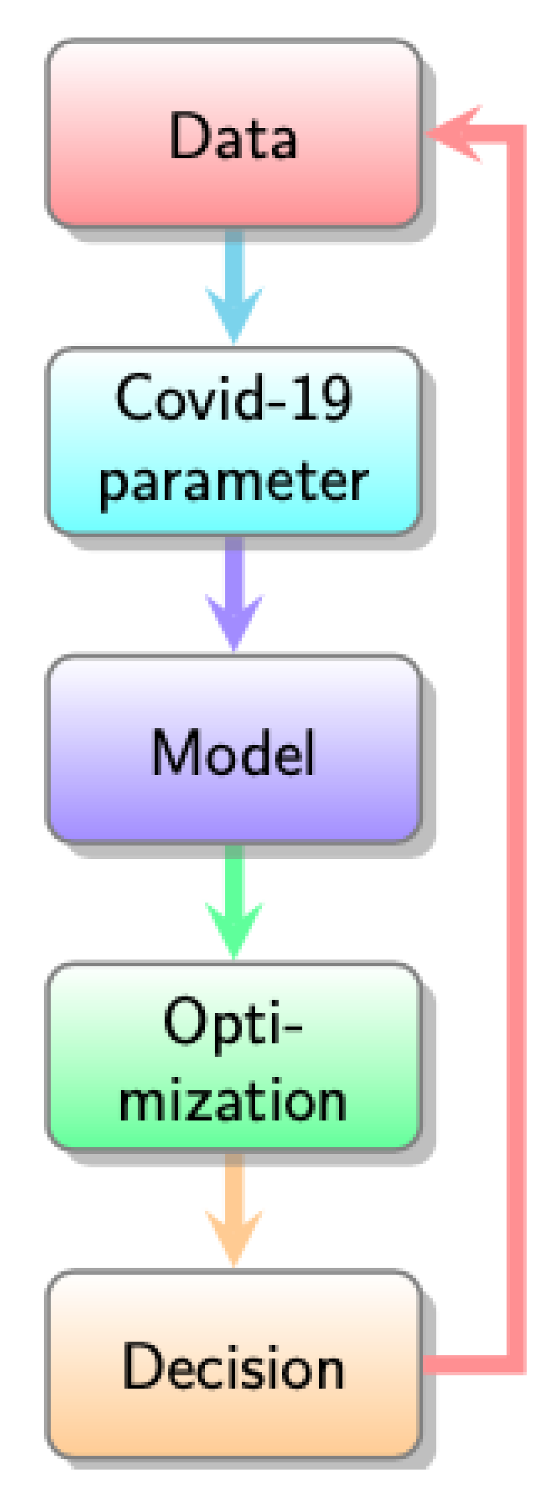
Figure 1.
Data-Driven MFTG Model: Data, Covid-19 parameter, Model, Optimization, Decision and back to the data measurement. The verification-validation procedure used in this article.
Figure 1.
Data-Driven MFTG Model: Data, Covid-19 parameter, Model, Optimization, Decision and back to the data measurement. The verification-validation procedure used in this article.
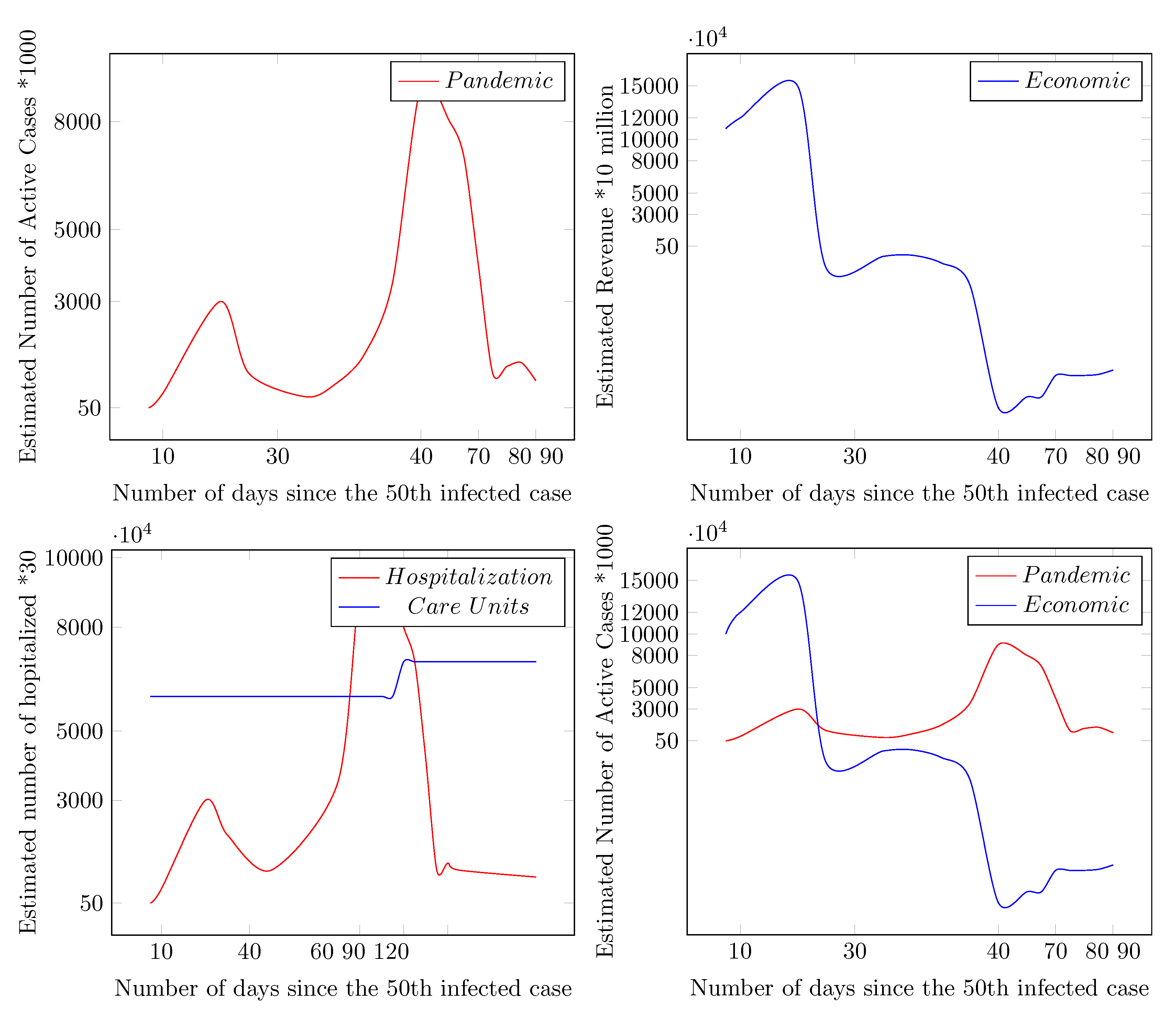
Figure 2.
Pandemic vs. Economic Consequences of COVID-19.
Figure 2.
Pandemic vs. Economic Consequences of COVID-19.
Figure 3.
First flow of infection of COVID-19 from Asia to Europe to America and then to Africa.
Figure 3.
First flow of infection of COVID-19 from Asia to Europe to America and then to Africa.
Figure 4.
Death rate distribution by age.
Figure 4.
Death rate distribution by age.
Figure 5.
A sample age distribution (unnormalized) for a specific sector.
Figure 5.
A sample age distribution (unnormalized) for a specific sector.
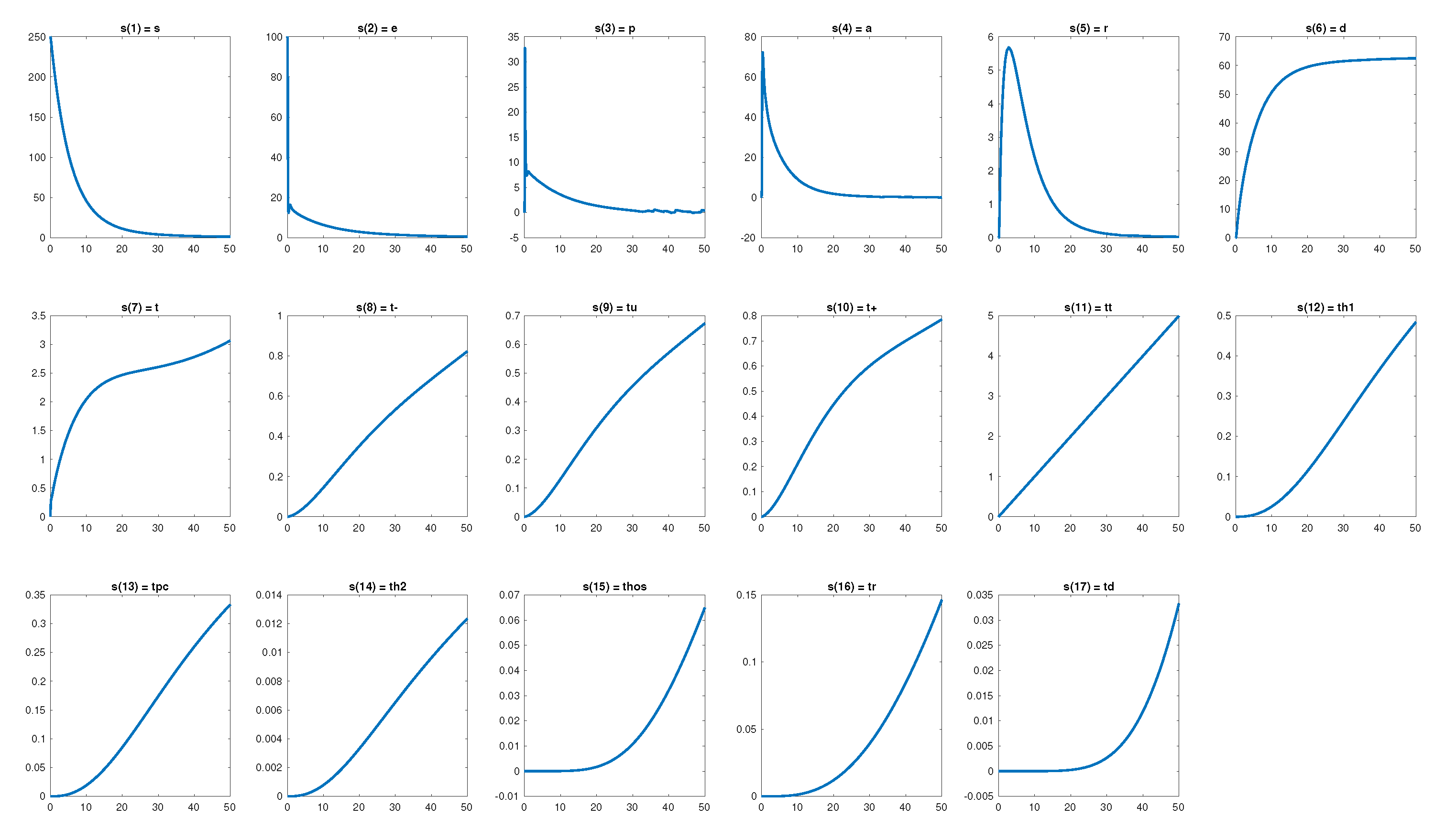
Figure 6.
Evolution of the ODE with 17 infection states.
Figure 6.
Evolution of the ODE with 17 infection states.
Figure 7.
Intra-dynamics at a given location with untested and tested options. Home, hotel, point-of-care isolation. l.a.c=location(l)-age (a)-pre-existing condition (c), gender, height, family size, economic status.
Figure 7.
Intra-dynamics at a given location with untested and tested options. Home, hotel, point-of-care isolation. l.a.c=location(l)-age (a)-pre-existing condition (c), gender, height, family size, economic status.
Figure 8.
Connection of the dynamics of SIR.
Figure 8.
Connection of the dynamics of SIR.
Figure 9.
Connection of the dynamics of SEIR.
Figure 9.
Connection of the dynamics of SEIR.
Figure 10.
Connection of the dynamics of SIRD.
Figure 10.
Connection of the dynamics of SIRD.
Figure 11.
Connection of the dynamics of SEIRD.
Figure 11.
Connection of the dynamics of SEIRD.
Figure 12.
World map: reported infectious as of 30 March 2020.
Figure 12.
World map: reported infectious as of 30 March 2020.
Figure 13.
Propagation of the virus in 15 most reported active cases as of 11 April 2020.
Figure 13.
Propagation of the virus in 15 most reported active cases as of 11 April 2020.
Figure 14.
COVID-19 samples in G7 countries.
Figure 14.
COVID-19 samples in G7 countries.
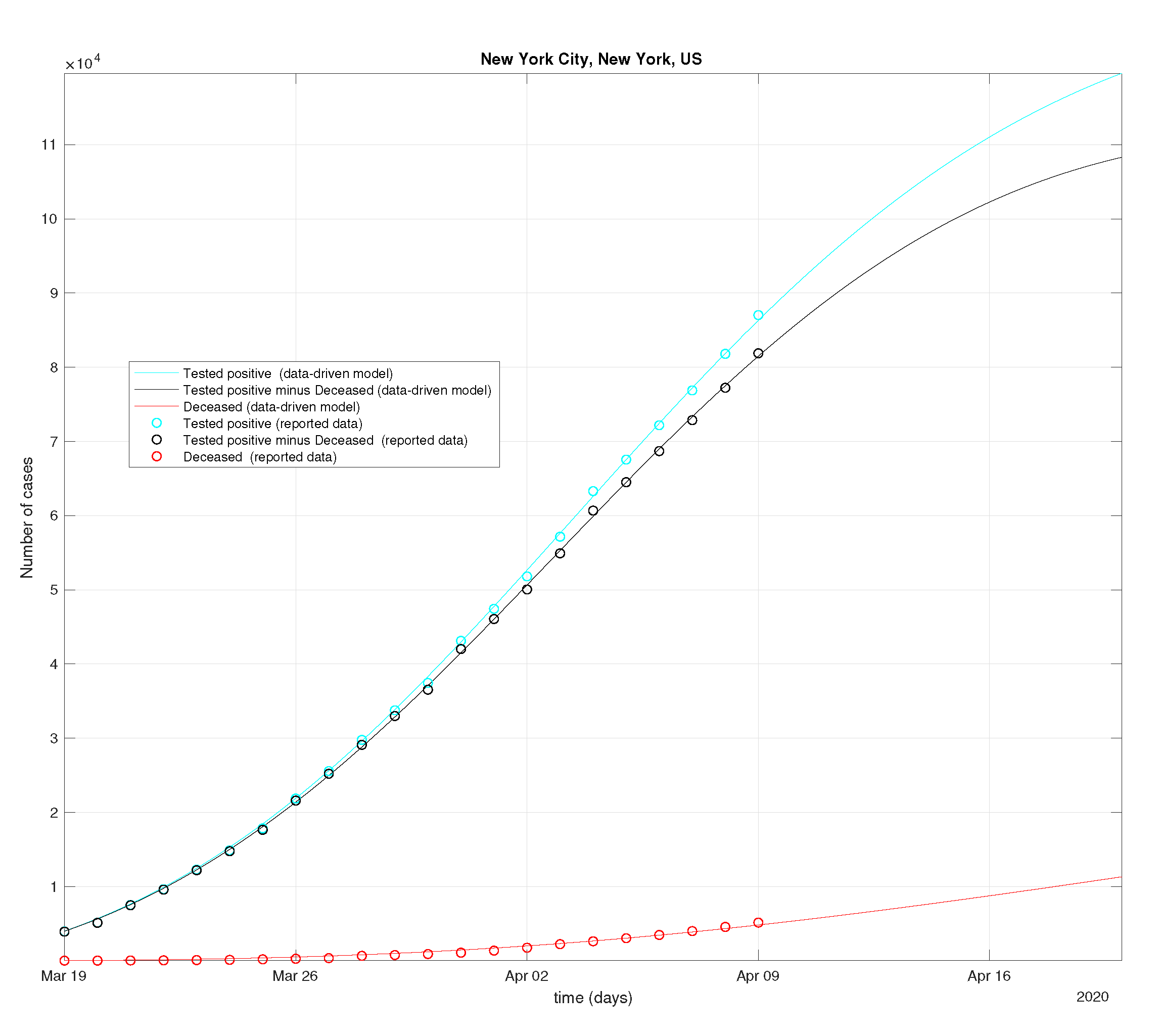
Figure 15.
New York and Los Angeles testing results: data vs. model.
Figure 15.
New York and Los Angeles testing results: data vs. model.
Figure 16.
COVID-19 sample of Non-Gaussianity and non-exponential. The plots are obtained by using the data set sequentially till the latest data point. A Non-Gaussianity of the reported active cases and hospitalized cases is observed. The shape of the sequential data-driven curve is clearly not a single exponential.
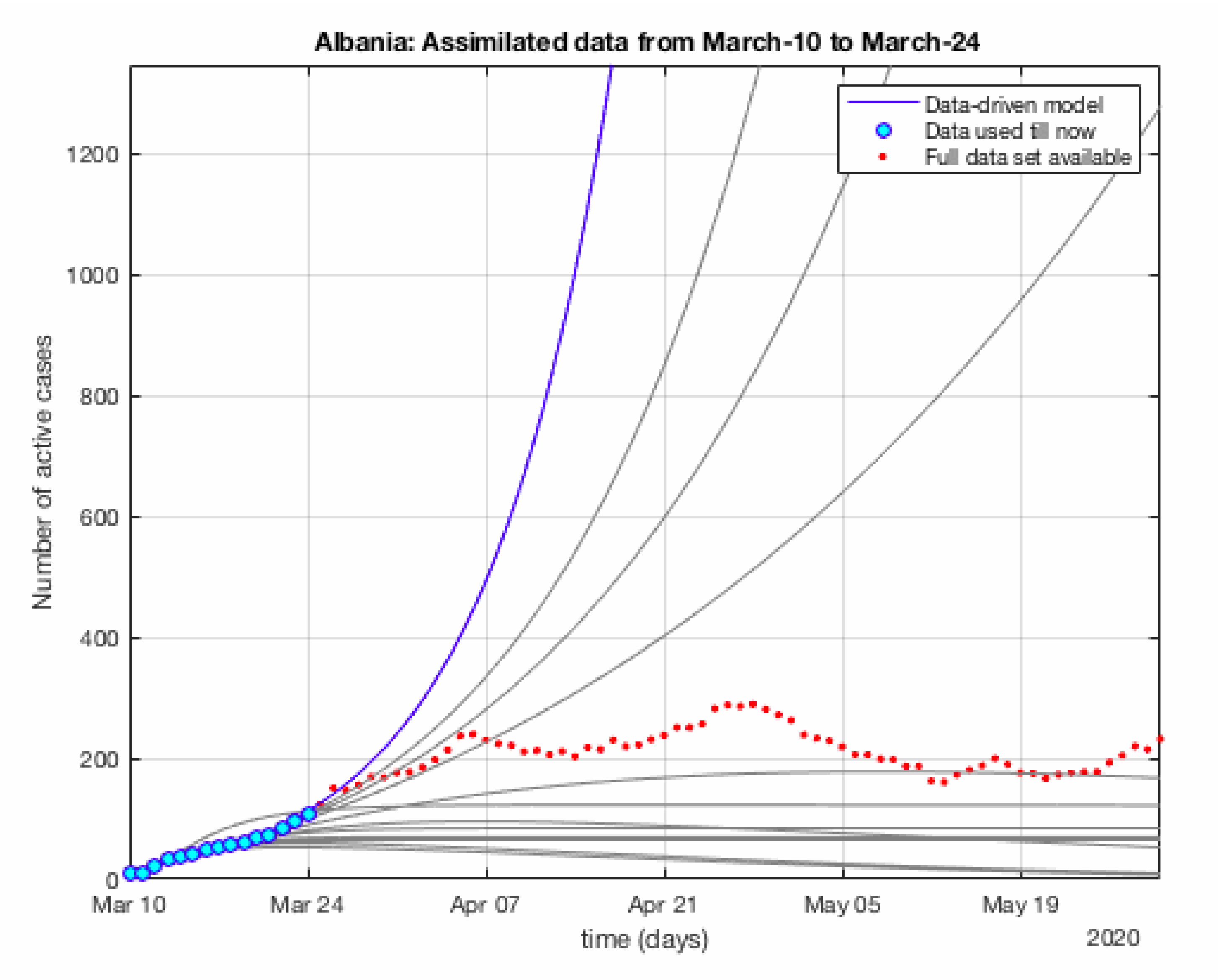
Figure 17.
Another COVID-19 sample of Non-Gaussianity and non-exponential. The plots are obtained by using the data set sequentially till the latest data point. A Non-Gaussianity of the reported active cases and hospitalized cases is observed. The shape of the sequential data-driven curve is clearly not a single exponential.
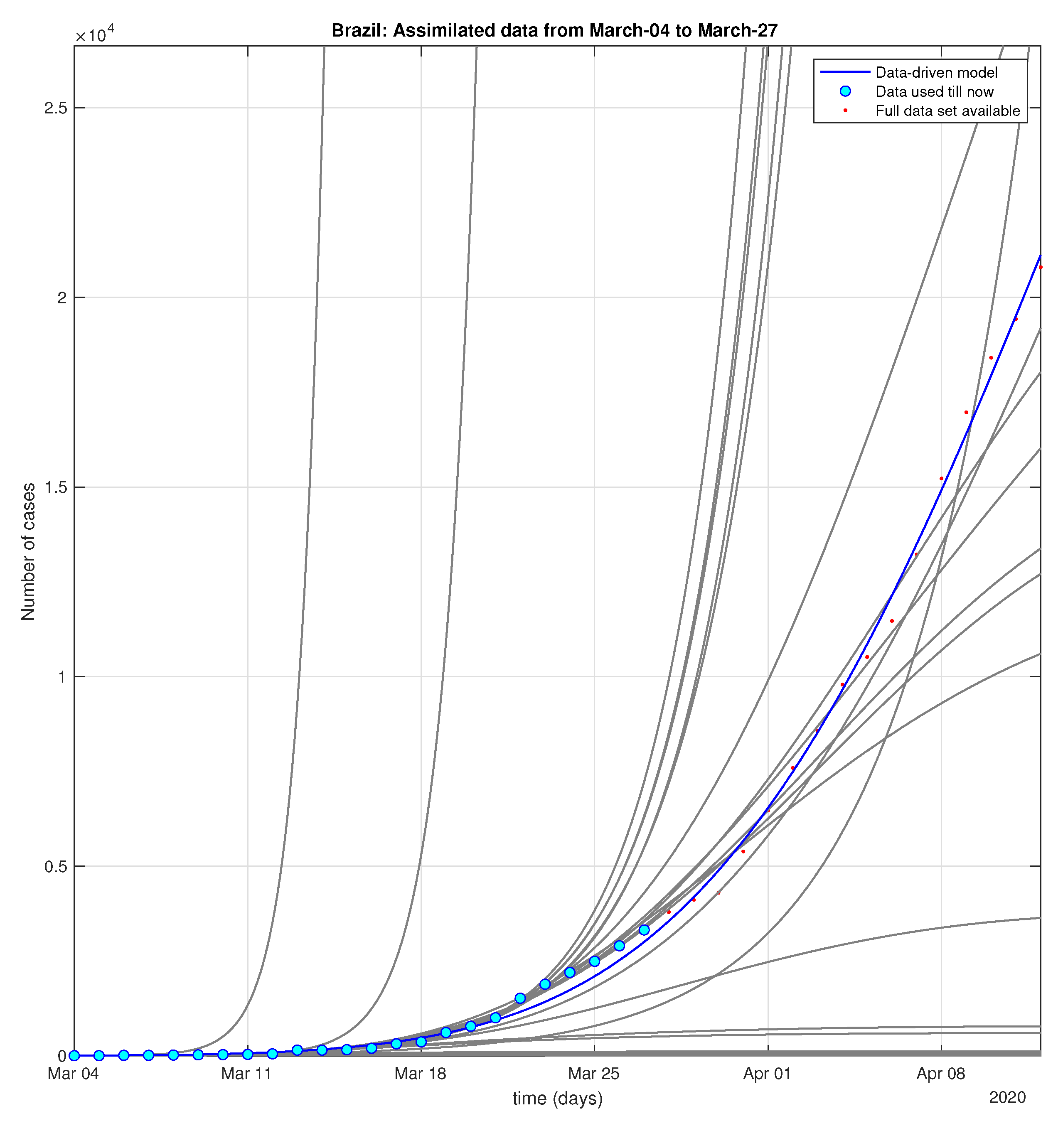
Figure 18.
Brazil: Sequential data-driven model.
Figure 18.
Brazil: Sequential data-driven model.
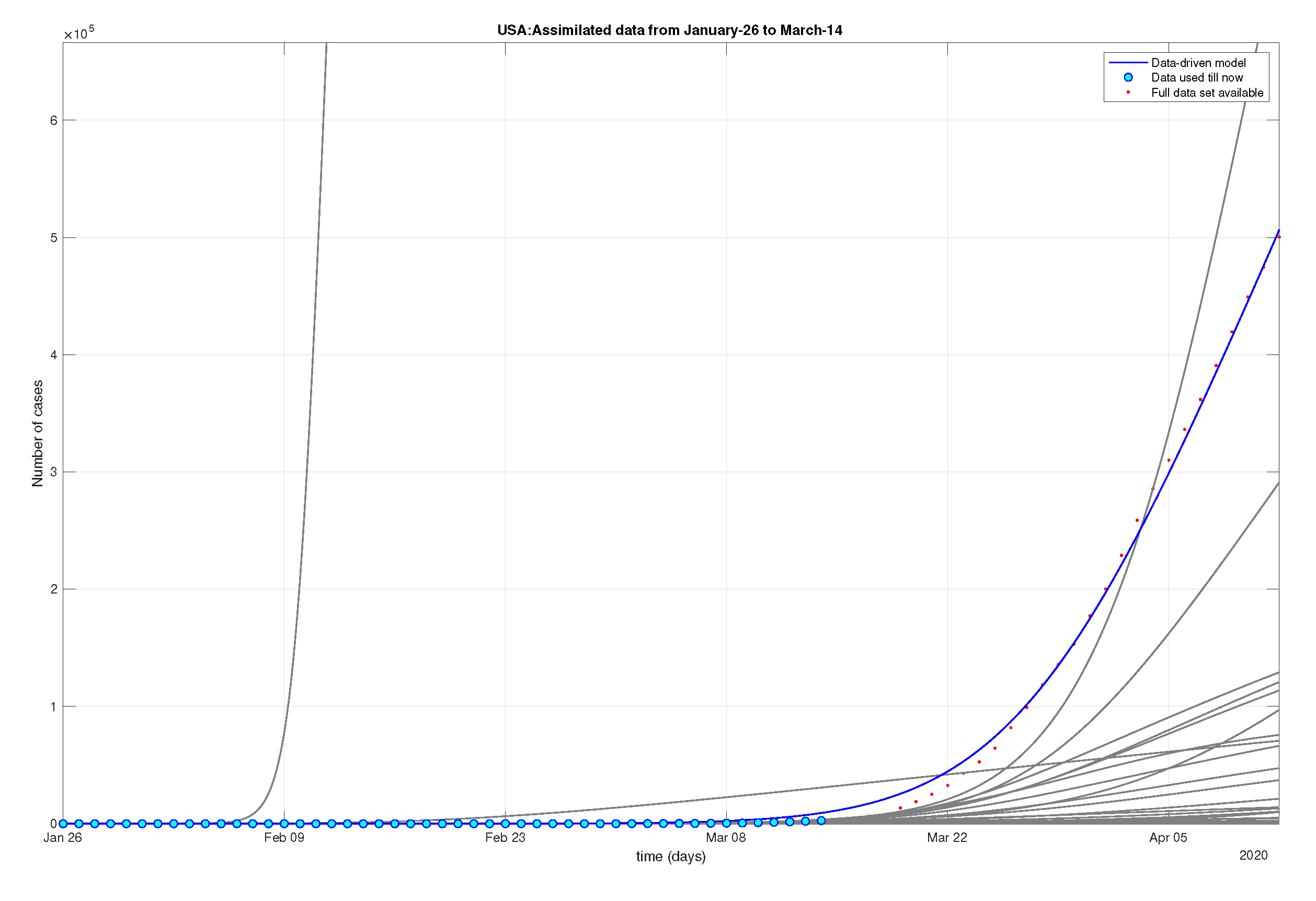
Figure 19.
USA: Sequential data-driven model.
Figure 19.
USA: Sequential data-driven model.
Figure 20.
Argentina: data of active, recovered, deceased (in circle or bar) vs. model of active, recovered, deceased over time. Tracking the number of active cases. Predictive analytics for the next couple days.
Figure 20.
Argentina: data of active, recovered, deceased (in circle or bar) vs. model of active, recovered, deceased over time. Tracking the number of active cases. Predictive analytics for the next couple days.
Figure 21.
Bolivia: data of active, recovered, deceased (in circle or bar) vs. model of active, recovered, deceased over time. Tracking the number of active cases. Predictive analytics for the next couple days.
Figure 21.
Bolivia: data of active, recovered, deceased (in circle or bar) vs. model of active, recovered, deceased over time. Tracking the number of active cases. Predictive analytics for the next couple days.
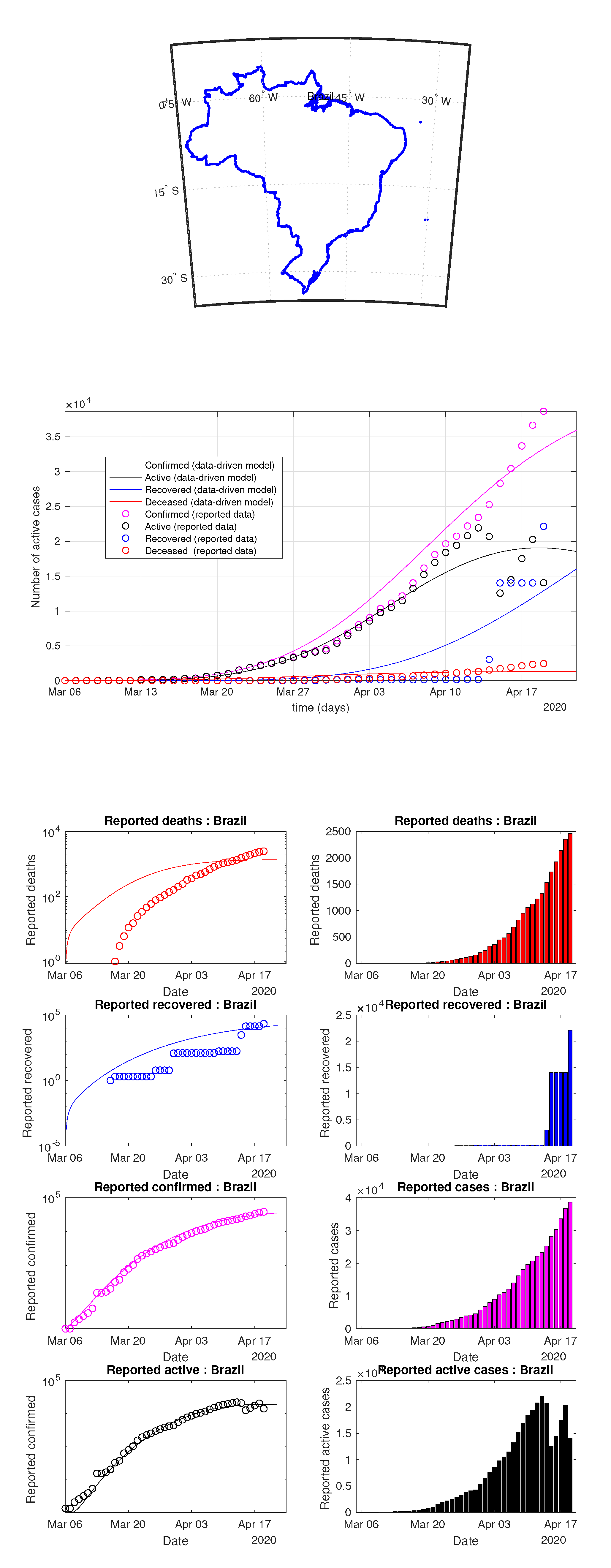
Figure 22.
Brazil: data of active, recovered, deceased (in circle or bar) vs. model of active, recovered, deceased over time. Tracking the number of active cases. Predictive analytics for the next couple days.
Figure 22.
Brazil: data of active, recovered, deceased (in circle or bar) vs. model of active, recovered, deceased over time. Tracking the number of active cases. Predictive analytics for the next couple days.
Figure 23.
Chile: data of active, recovered, deceased (in circle or bar) vs. model of active, recovered, deceased over time. Tracking the number of active cases. Predictive analytics for the next couple days.
Figure 23.
Chile: data of active, recovered, deceased (in circle or bar) vs. model of active, recovered, deceased over time. Tracking the number of active cases. Predictive analytics for the next couple days.
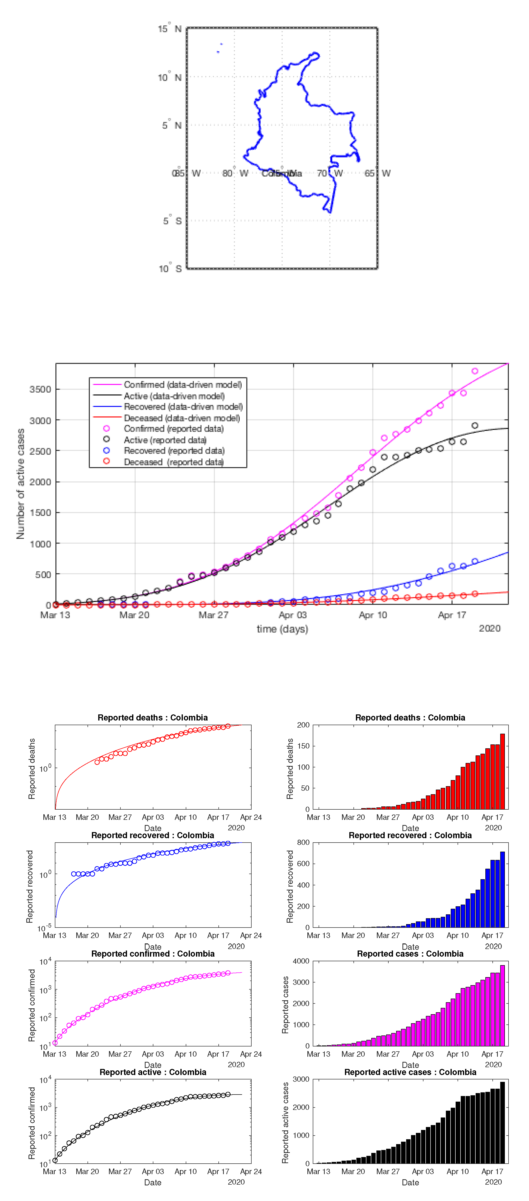
Figure 24.
Colombia: data of active, recovered, deceased (in circle or bar) vs. model of active, recovered, deceased over time. Tracking the number of active cases. Predictive analytics for the next couple days.
Figure 24.
Colombia: data of active, recovered, deceased (in circle or bar) vs. model of active, recovered, deceased over time. Tracking the number of active cases. Predictive analytics for the next couple days.
Figure 25.
Ecuador: data of active, recovered, deceased (in circle or bar) vs. model of active, recovered, deceased over time. Tracking the number of active cases. Predictive analytics for the next couple days.
Figure 25.
Ecuador: data of active, recovered, deceased (in circle or bar) vs. model of active, recovered, deceased over time. Tracking the number of active cases. Predictive analytics for the next couple days.
Figure 26.
Paraguay: data of active, recovered, deceased (in circle or bar) vs. model of active, recovered, deceased over time. Tracking the number of active cases. Predictive analytics for the next couple days.
Figure 26.
Paraguay: data of active, recovered, deceased (in circle or bar) vs. model of active, recovered, deceased over time. Tracking the number of active cases. Predictive analytics for the next couple days.
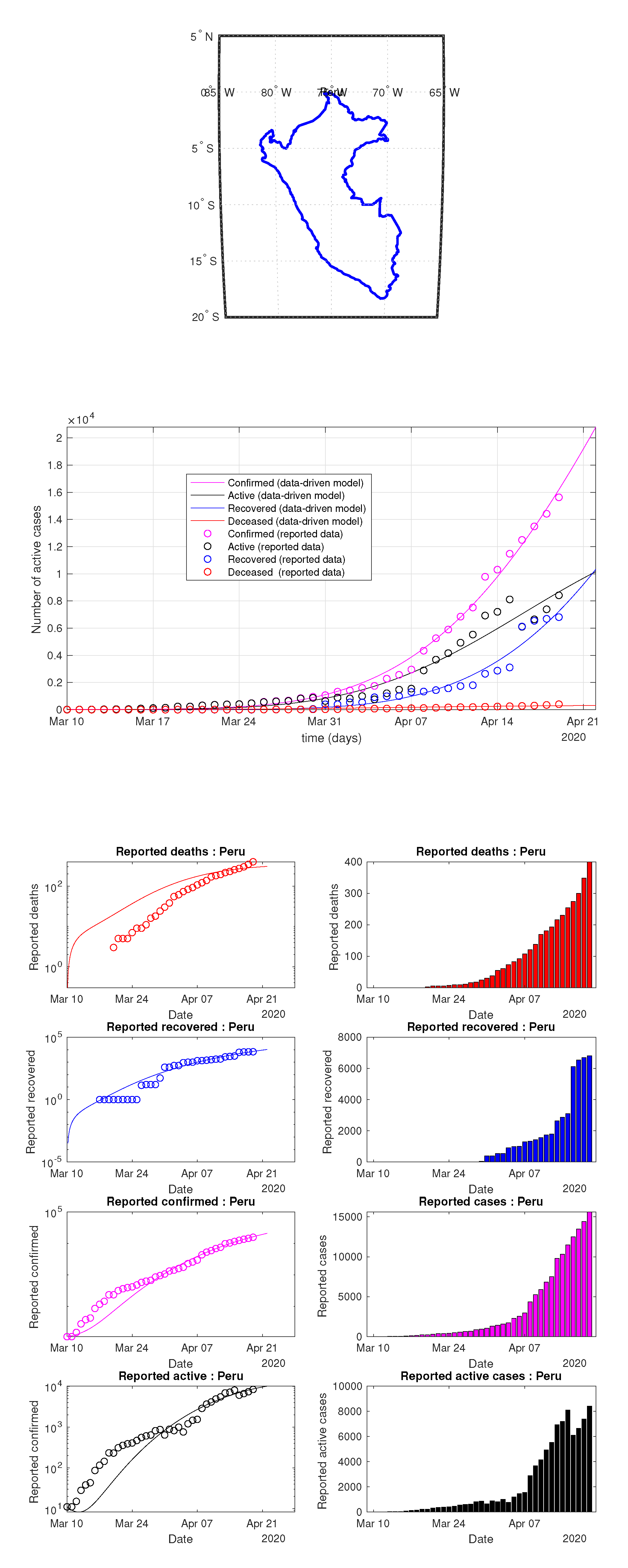
Figure 27.
Peru: data of active, recovered, deceased (in circle or bar) vs. model of active, recovered, deceased over time. Tracking the number of active cases. Predictive analytics for the next couple days.
Figure 27.
Peru: data of active, recovered, deceased (in circle or bar) vs. model of active, recovered, deceased over time. Tracking the number of active cases. Predictive analytics for the next couple days.
Figure 28.
Uruguay: data of active, recovered, deceased (in circle or bar) vs. model of active, recovered, deceased over time. Tracking the number of active cases. Predictive analytics for the next couple days.
Figure 28.
Uruguay: data of active, recovered, deceased (in circle or bar) vs. model of active, recovered, deceased over time. Tracking the number of active cases. Predictive analytics for the next couple days.
Figure 29.
Venezuela: data of active, recovered, deceased (in circle or bar) vs. model of active, recovered, deceased over time. Tracking the number of active cases. Predictive analytics for the next couple days.
Figure 29.
Venezuela: data of active, recovered, deceased (in circle or bar) vs. model of active, recovered, deceased over time. Tracking the number of active cases. Predictive analytics for the next couple days.
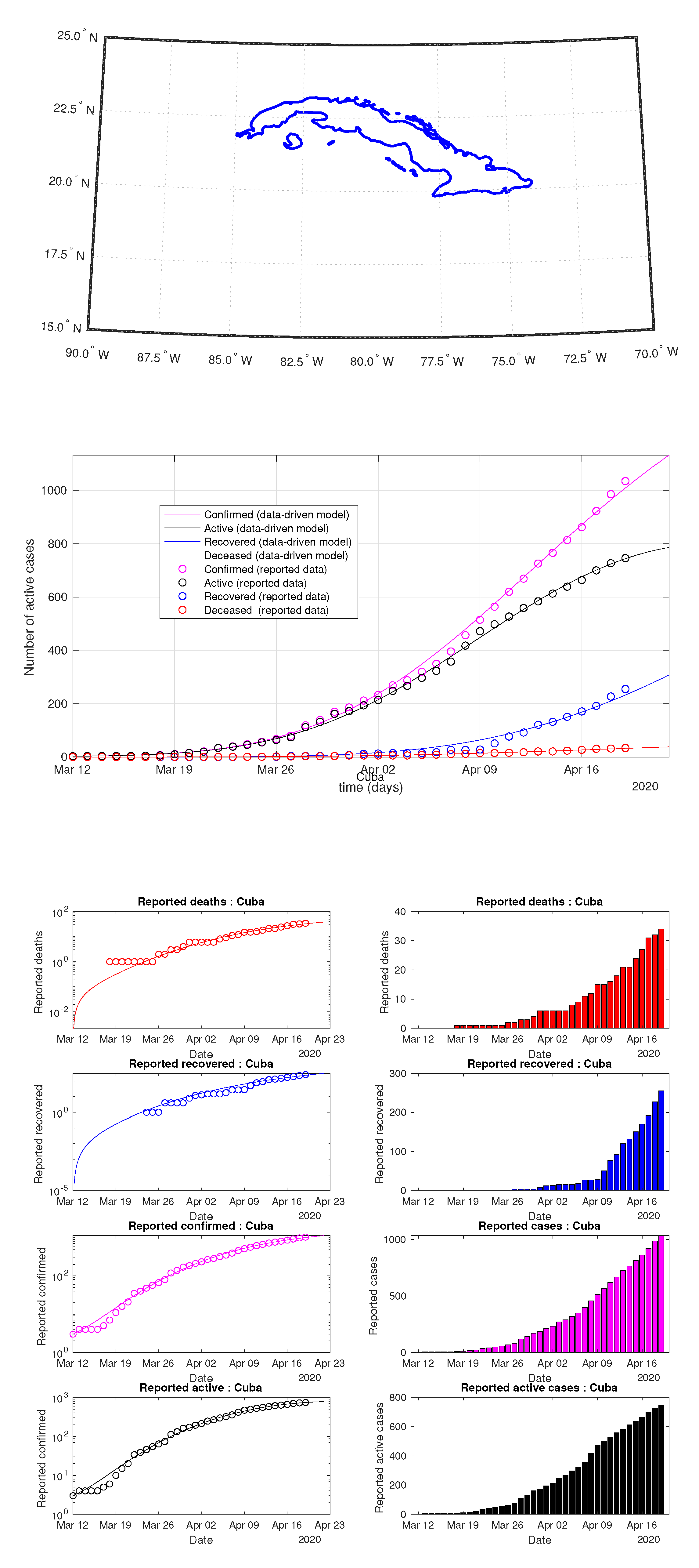
Figure 30.
Cuba: data of active, recovered, deceased (in circle or bar) vs. model of active, recovered, deceased over time. Tracking the number of active cases. Predictive analytics for the next couple days.
Figure 30.
Cuba: data of active, recovered, deceased (in circle or bar) vs. model of active, recovered, deceased over time. Tracking the number of active cases. Predictive analytics for the next couple days.
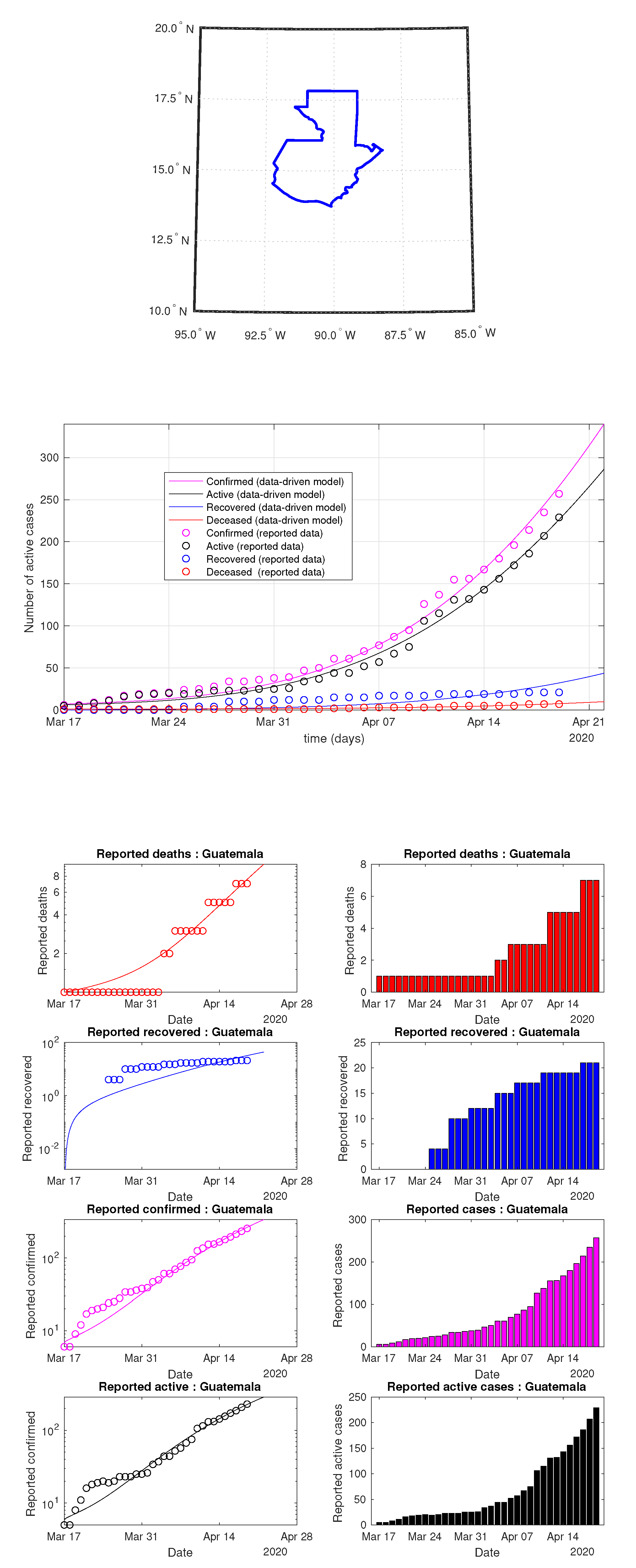
Figure 31.
Guatemala: data of active, recovered, deceased (in circle or bar) vs. model of active, recovered, deceased over time. Tracking the number of active cases. Predictive analytics for the next couple days.
Figure 31.
Guatemala: data of active, recovered, deceased (in circle or bar) vs. model of active, recovered, deceased over time. Tracking the number of active cases. Predictive analytics for the next couple days.
Figure 32.
Haiti: data of active, recovered, deceased (in circle or bar) vs. model of active, recovered, deceased over time. Tracking the number of active cases. Predictive analytics for the next couple days.
Figure 32.
Haiti: data of active, recovered, deceased (in circle or bar) vs. model of active, recovered, deceased over time. Tracking the number of active cases. Predictive analytics for the next couple days.
Figure 33.
Mexico: data of active, recovered, deceased (in circle or bar) vs. model of active, recovered, deceased over time. Tracking the number of active cases over time. Predictive analytics for the next couple days.
Figure 33.
Mexico: data of active, recovered, deceased (in circle or bar) vs. model of active, recovered, deceased over time. Tracking the number of active cases over time. Predictive analytics for the next couple days.
Figure 34.
Bangladesh: data of active, recovered, deceased (in circle or bar) vs. model of active, recovered, deceased over time. Tracking the number of active cases. Predictive analytics for the next couple days.
Figure 34.
Bangladesh: data of active, recovered, deceased (in circle or bar) vs. model of active, recovered, deceased over time. Tracking the number of active cases. Predictive analytics for the next couple days.
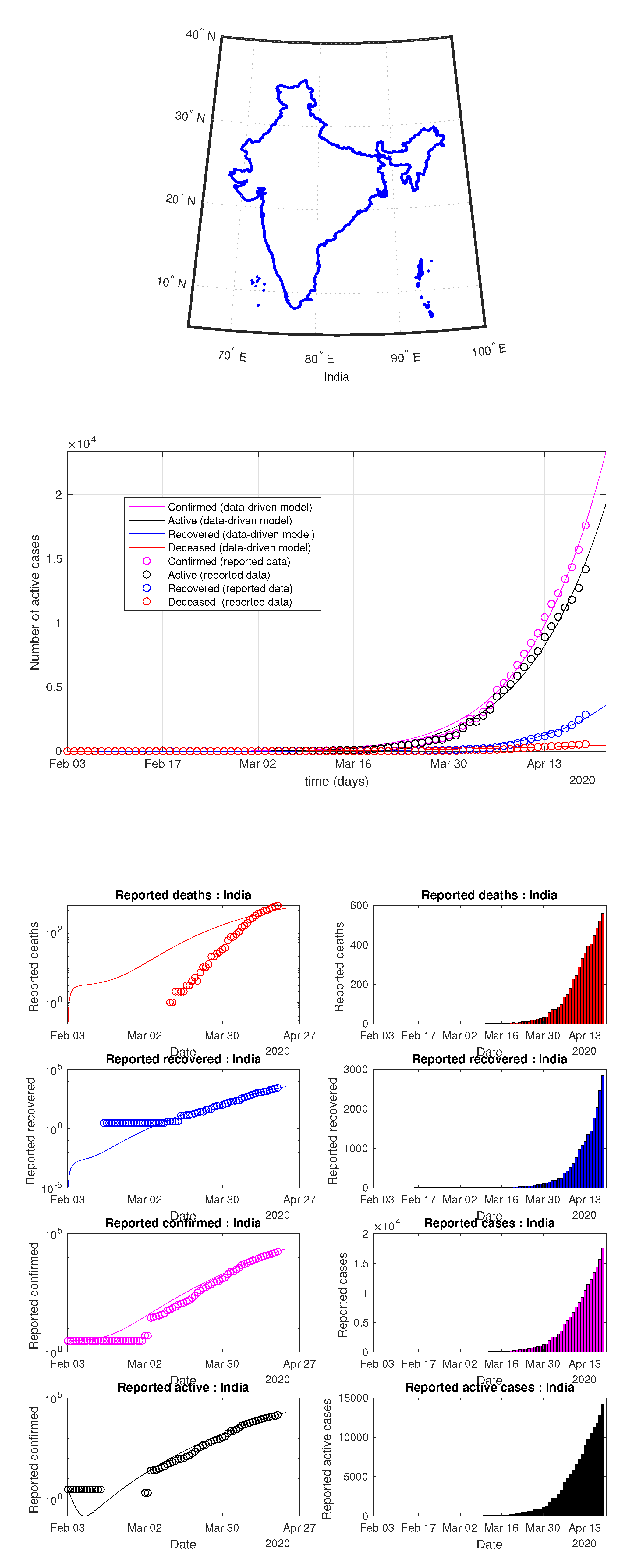
Figure 35.
India: data of active, recovered, deceased (in circle or bar) vs. model of active, recovered, deceased over time. Tracking the number of active cases. Predictive analytics for the next couple days.
Figure 35.
India: data of active, recovered, deceased (in circle or bar) vs. model of active, recovered, deceased over time. Tracking the number of active cases. Predictive analytics for the next couple days.
Figure 36.
Indonesia: data of active, recovered, deceased (in circle or bar) vs. model of active, recovered, deceased over time. Tracking the number of active cases. Predictive analytics for the next couple days.
Figure 36.
Indonesia: data of active, recovered, deceased (in circle or bar) vs. model of active, recovered, deceased over time. Tracking the number of active cases. Predictive analytics for the next couple days.
Figure 37.
South Korea: data of active, recovered, deceased (in circle or bar) vs. model of active, recovered, deceased over time. Tracking the number of active cases. Predictive analytics for the next couple days.
Figure 37.
South Korea: data of active, recovered, deceased (in circle or bar) vs. model of active, recovered, deceased over time. Tracking the number of active cases. Predictive analytics for the next couple days.
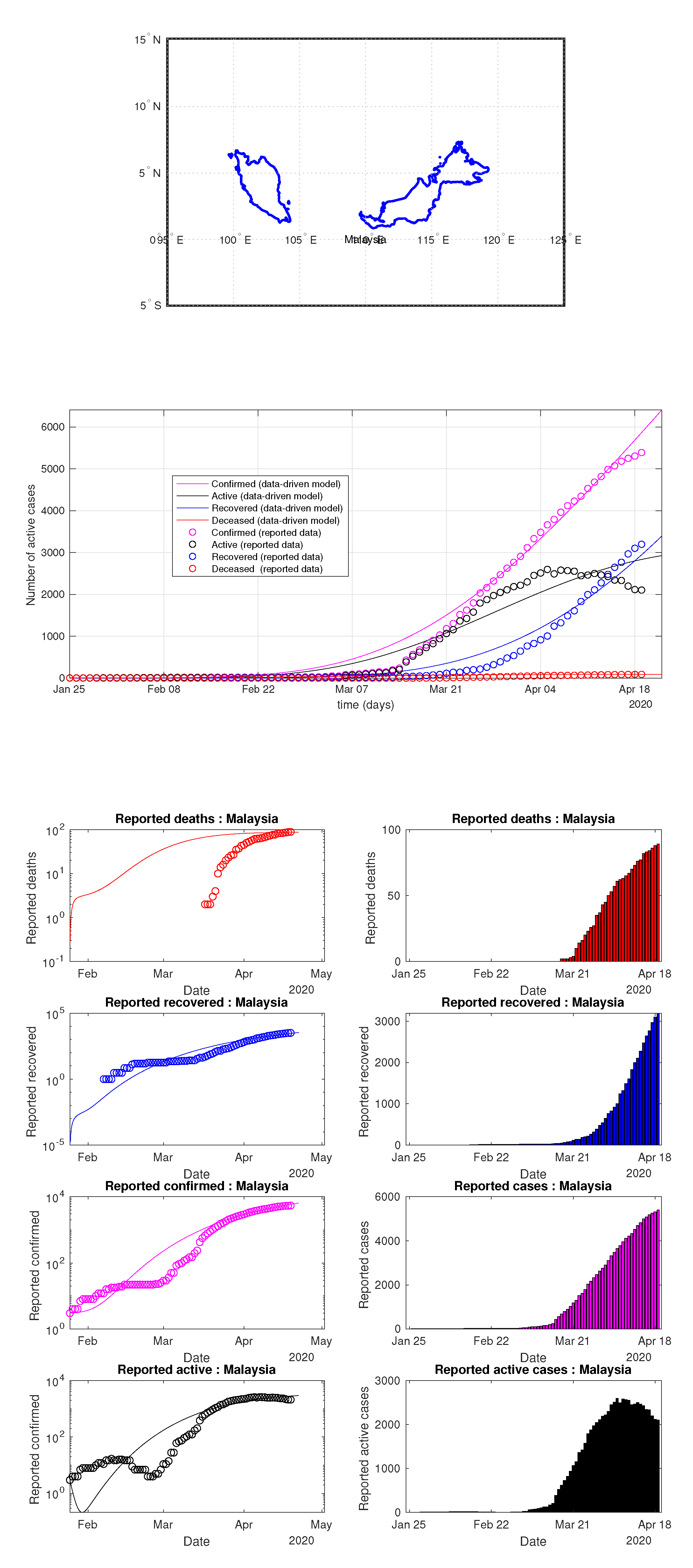
Figure 38.
Malaysia: data of active, recovered, deceased (in circle or bar) vs. model of active, recovered, deceased over time. Tracking the number of active cases. Predictive analytics for the next couple days.
Figure 38.
Malaysia: data of active, recovered, deceased (in circle or bar) vs. model of active, recovered, deceased over time. Tracking the number of active cases. Predictive analytics for the next couple days.
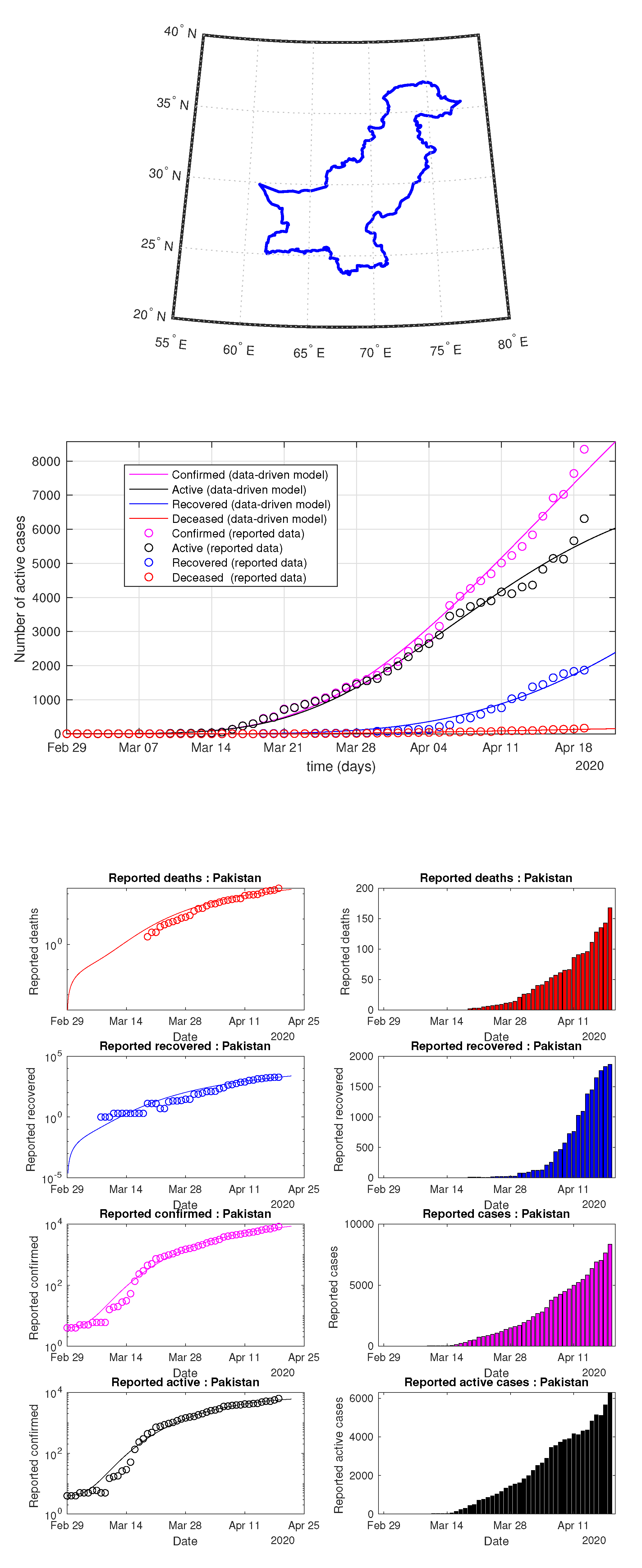
Figure 39.
Pakistan: data of active, recovered, deceased (in circle or bar) vs. model of active, recovered, deceased over time. Tracking the number of active cases. Predictive analytics for the next couple days.
Figure 39.
Pakistan: data of active, recovered, deceased (in circle or bar) vs. model of active, recovered, deceased over time. Tracking the number of active cases. Predictive analytics for the next couple days.
Figure 40.
UAE: data of active, recovered, deceased (in circle or bar) vs. model of active, recovered, deceased over time. Tracking the number of active cases. Predictive analytics for the next couple days.
Figure 40.
UAE: data of active, recovered, deceased (in circle or bar) vs. model of active, recovered, deceased over time. Tracking the number of active cases. Predictive analytics for the next couple days.
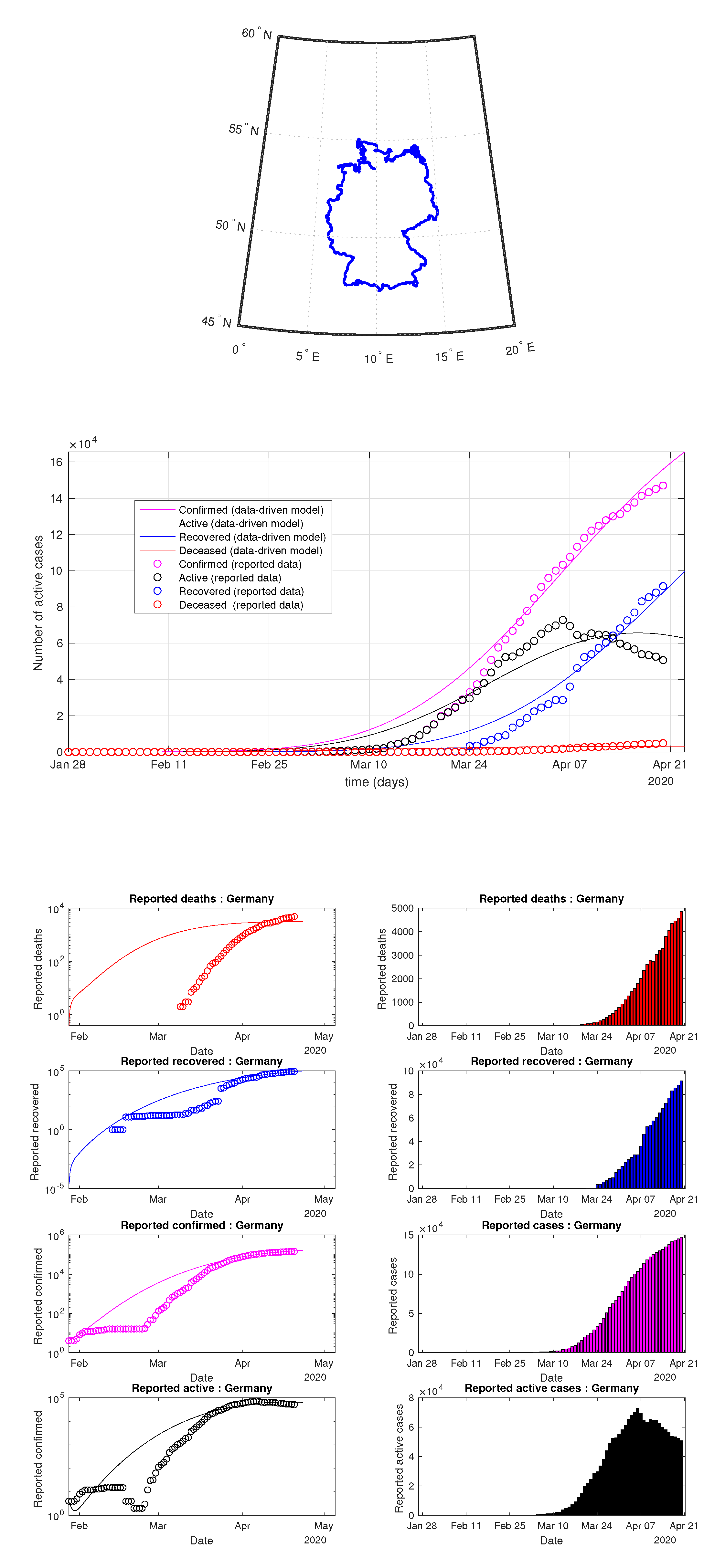
Figure 41.
Germany: data of active, recovered, deceased (in circle or bar) vs. model of active, recovered, deceased over time. Tracking the number of active cases. Predictive analytics for the next couple days.
Figure 41.
Germany: data of active, recovered, deceased (in circle or bar) vs. model of active, recovered, deceased over time. Tracking the number of active cases. Predictive analytics for the next couple days.
Figure 42.
Italy: data of active, recovered, deceased (in circle or bar) vs. model of active, recovered, deceased over time. Tracking the number of active cases. Predictive analytics for the next couple days.
Figure 42.
Italy: data of active, recovered, deceased (in circle or bar) vs. model of active, recovered, deceased over time. Tracking the number of active cases. Predictive analytics for the next couple days.
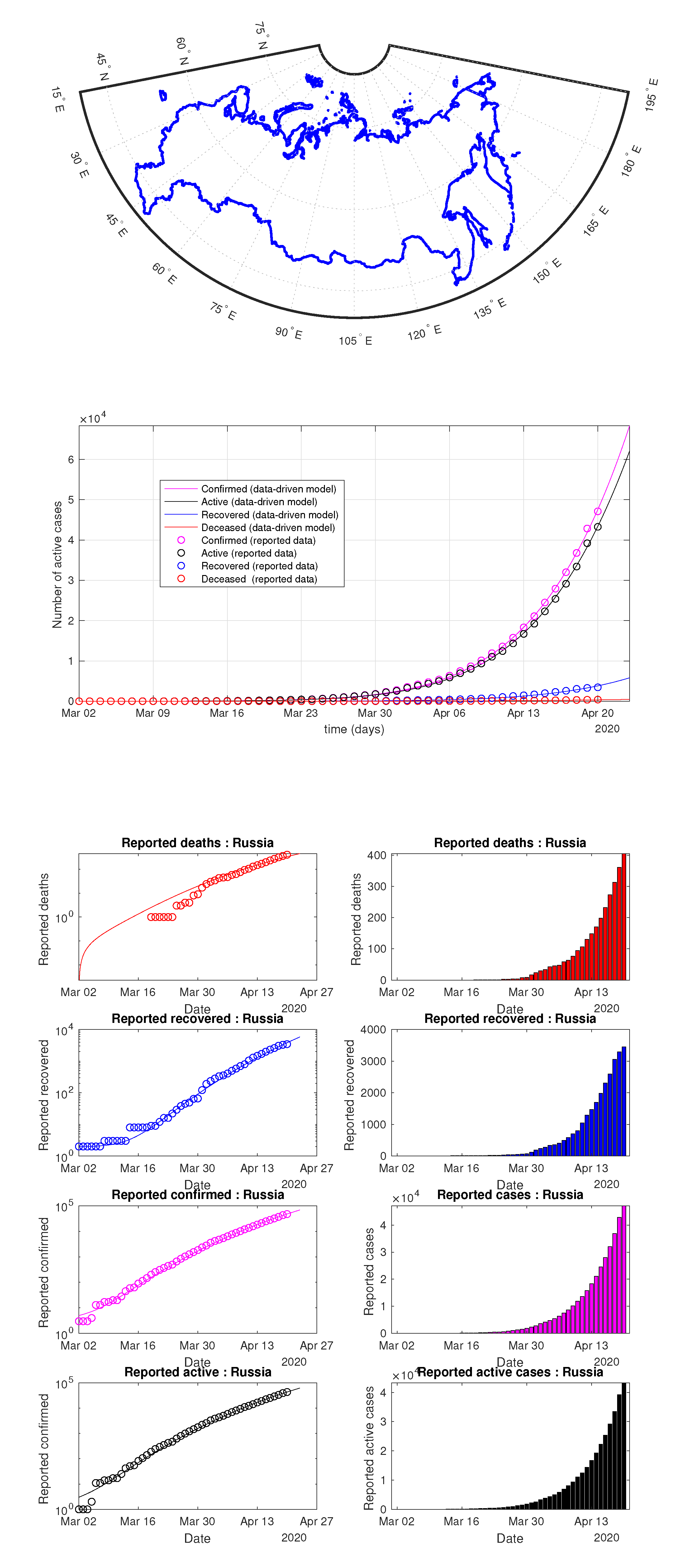
Figure 43.
Russia: data of active, recovered, deceased (in circle or bar) vs. model of active, recovered, deceased over time. Tracking the number of active cases. Predictive analytics for the next couple days.
Figure 43.
Russia: data of active, recovered, deceased (in circle or bar) vs. model of active, recovered, deceased over time. Tracking the number of active cases. Predictive analytics for the next couple days.
Figure 44.
Spain: data of active, recovered, deceased (in circle or bar) vs. model of active, recovered, deceased over time. Tracking the number of active cases. Predictive analytics for the next couple days.
Figure 44.
Spain: data of active, recovered, deceased (in circle or bar) vs. model of active, recovered, deceased over time. Tracking the number of active cases. Predictive analytics for the next couple days.
Figure 45.
Covid-19 samples in selected countries in Africa
Figure 45.
Covid-19 samples in selected countries in Africa
Figure 46.
Selected COMESA countries
Figure 46.
Selected COMESA countries
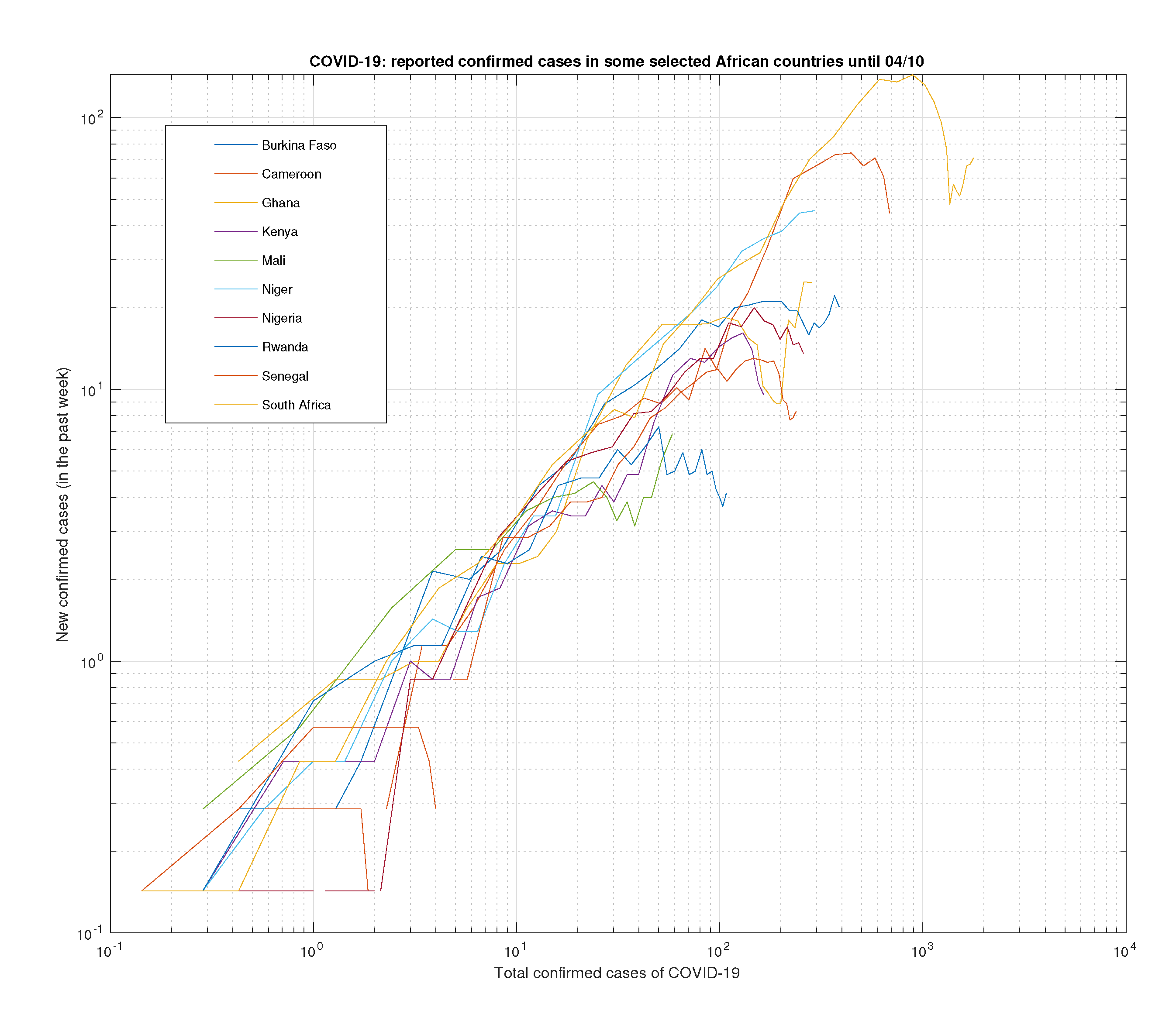
Figure 47.
Selected ECOWAS countries.
Figure 47.
Selected ECOWAS countries.
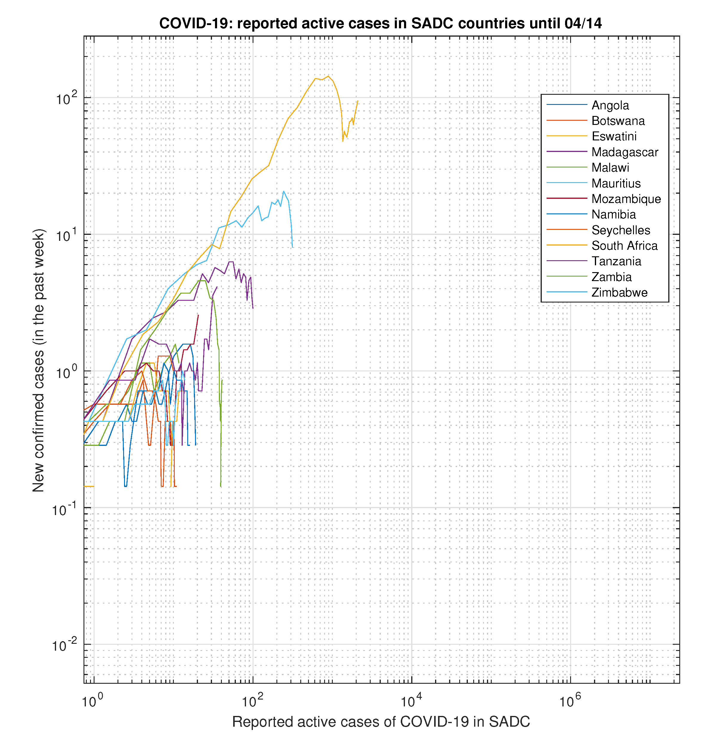
Figure 48.
Selected SADC countries.
Figure 48.
Selected SADC countries.
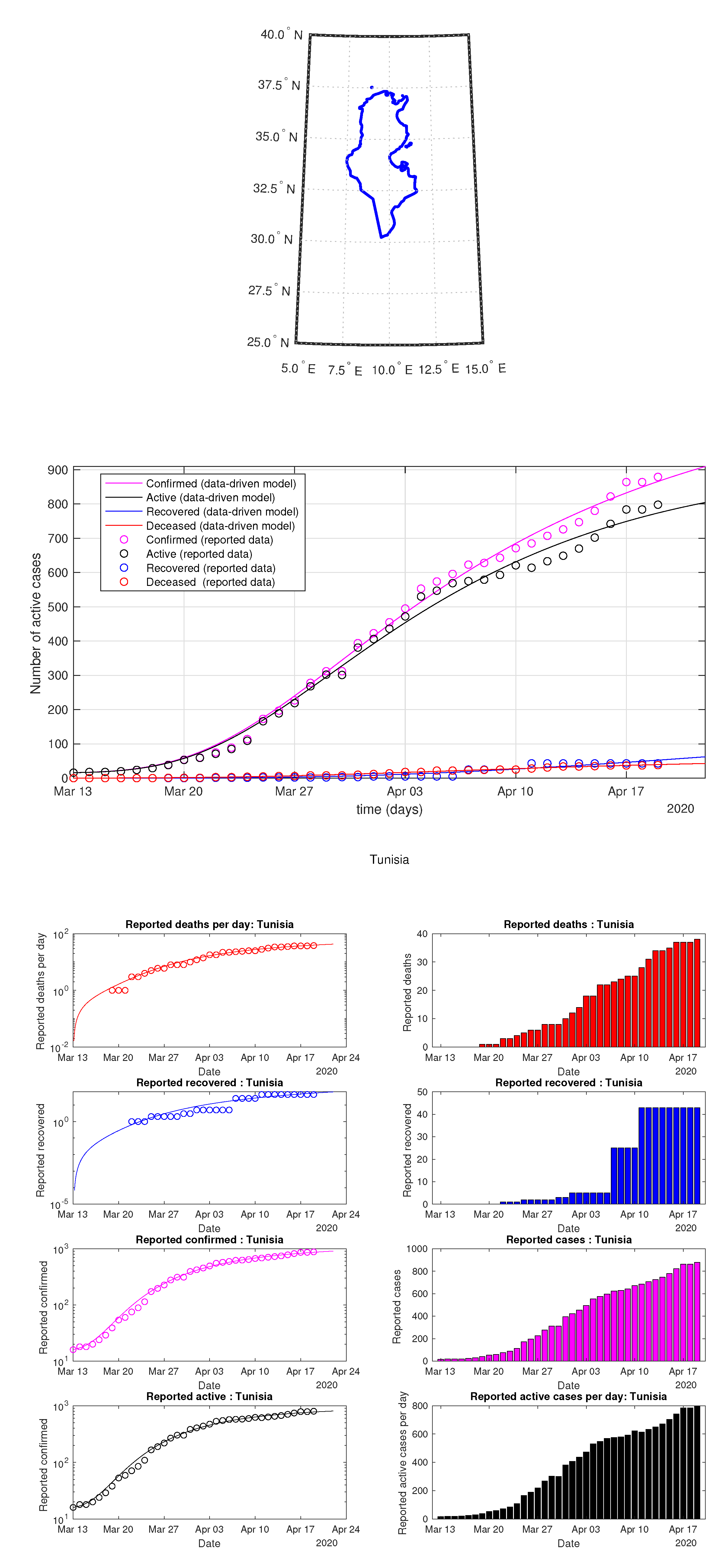
Figure 49.
Tunisia: Sequential data-driven model
Figure 49.
Tunisia: Sequential data-driven model
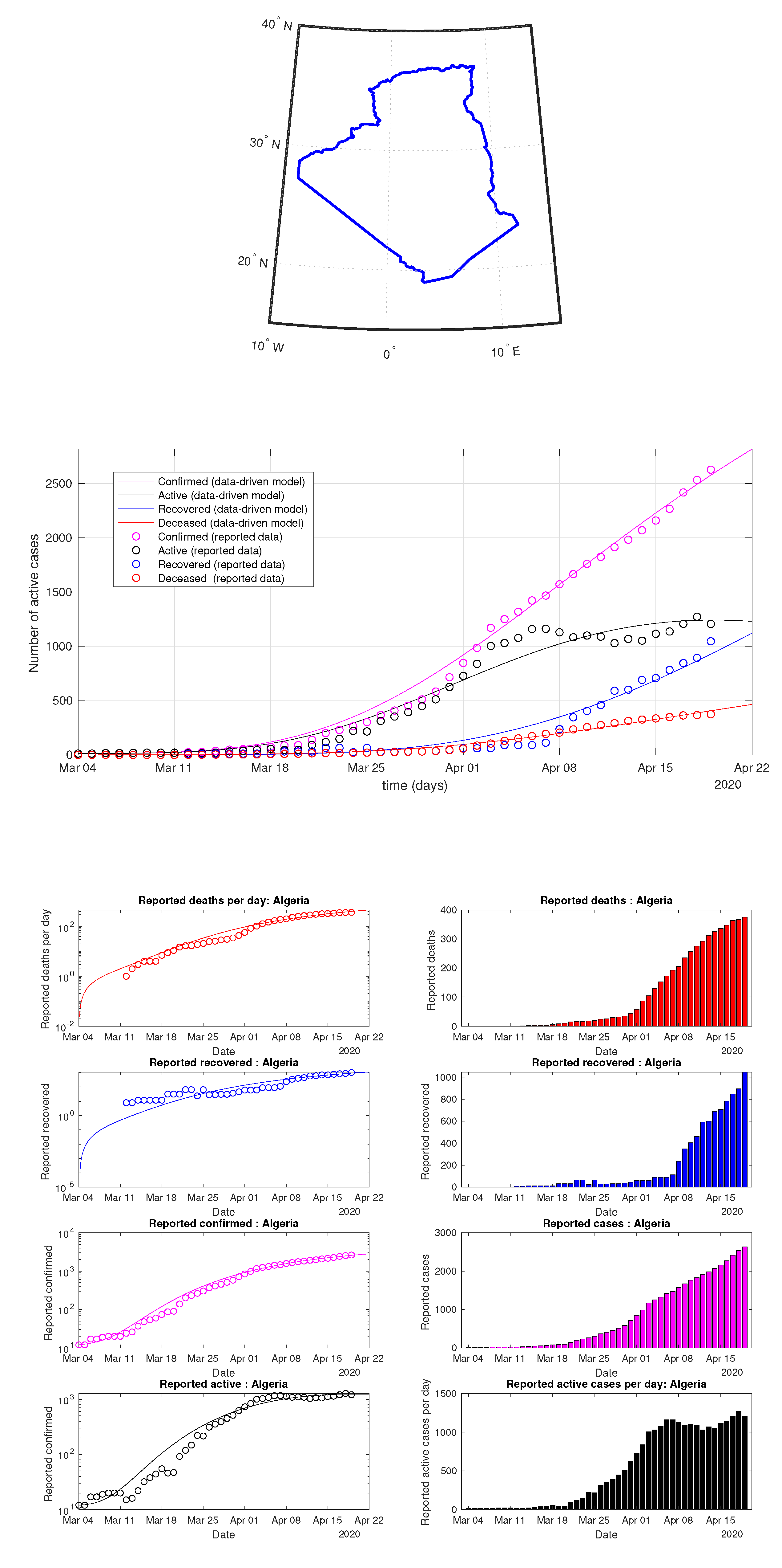
Figure 50.
Algeria: data of active, recovered, deceased (in circle or bar) vs. model of active, recovered, deceased over time. Tracking the number of active cases. Predictive analytics for the next couple days.
Figure 50.
Algeria: data of active, recovered, deceased (in circle or bar) vs. model of active, recovered, deceased over time. Tracking the number of active cases. Predictive analytics for the next couple days.
Figure 51.
Angola: data of active, recovered, deceased (in circle or bar) vs. model of active, recovered, deceased over time. Tracking the number of active cases. Predictive analytics for the next couple days.
Figure 51.
Angola: data of active, recovered, deceased (in circle or bar) vs. model of active, recovered, deceased over time. Tracking the number of active cases. Predictive analytics for the next couple days.
Figure 52.
Botswana: data of active, recovered, deceased (in circle or bar) vs. model of active, recovered, deceased over time. Tracking the number of active cases. Predictive analytics for the next couple days.
Figure 52.
Botswana: data of active, recovered, deceased (in circle or bar) vs. model of active, recovered, deceased over time. Tracking the number of active cases. Predictive analytics for the next couple days.
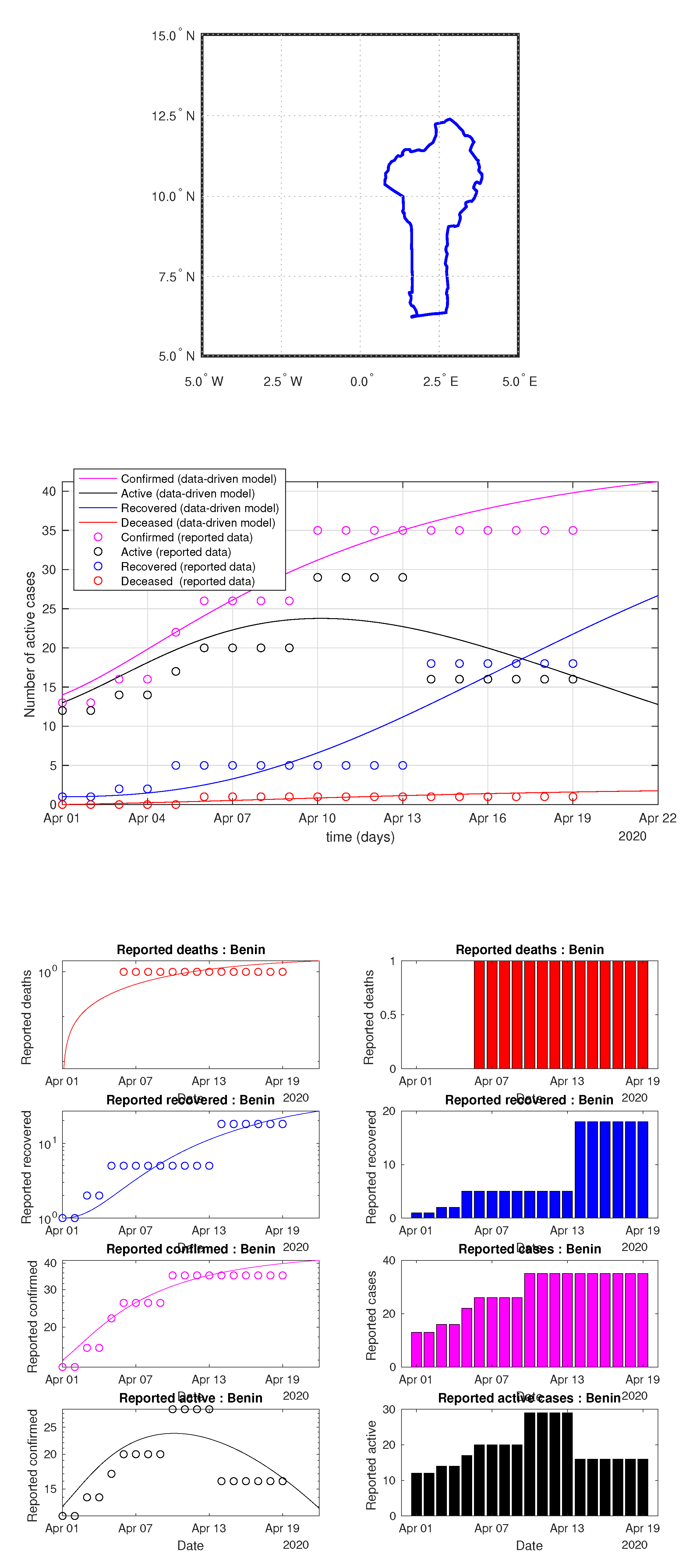
Figure 53.
Benin: data of active, recovered, deceased (in circle or bar) vs. model of active, recovered, deceased over time. Tracking the number of active cases. Predictive analytics for the next couple days.
Figure 53.
Benin: data of active, recovered, deceased (in circle or bar) vs. model of active, recovered, deceased over time. Tracking the number of active cases. Predictive analytics for the next couple days.
Figure 54.
Burkina Faso: data of active, recovered, deceased (in circle or bar) vs. model of active, recovered, deceased over time. Tracking the number of active cases. Predictive analytics for the next couple days.
Figure 54.
Burkina Faso: data of active, recovered, deceased (in circle or bar) vs. model of active, recovered, deceased over time. Tracking the number of active cases. Predictive analytics for the next couple days.
Figure 55.
Burundi: data of active, recovered, deceased (in circle or bar) vs. model of active, recovered, deceased over time. Tracking the number of active cases. Predictive analytics for the next couple days.
Figure 55.
Burundi: data of active, recovered, deceased (in circle or bar) vs. model of active, recovered, deceased over time. Tracking the number of active cases. Predictive analytics for the next couple days.
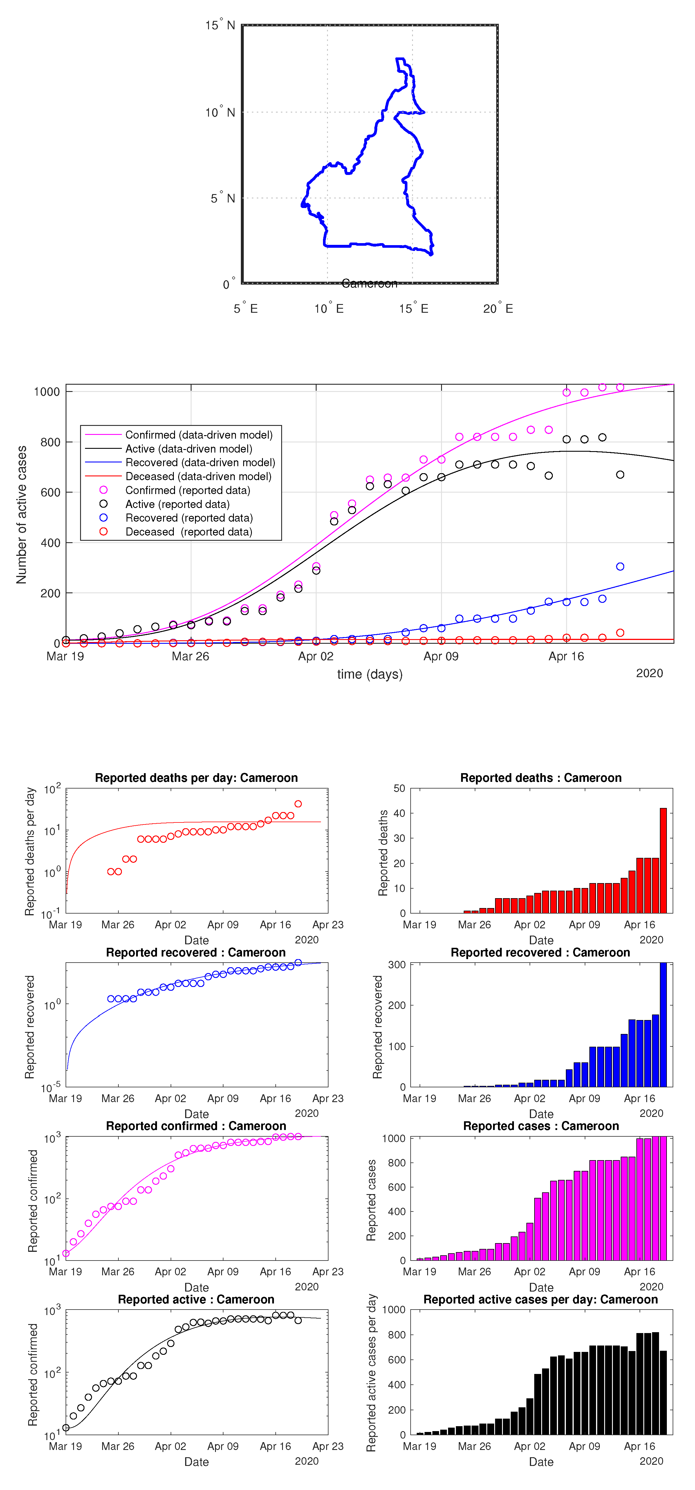
Figure 56.
Cameroon: data vs. model.
Figure 56.
Cameroon: data vs. model.
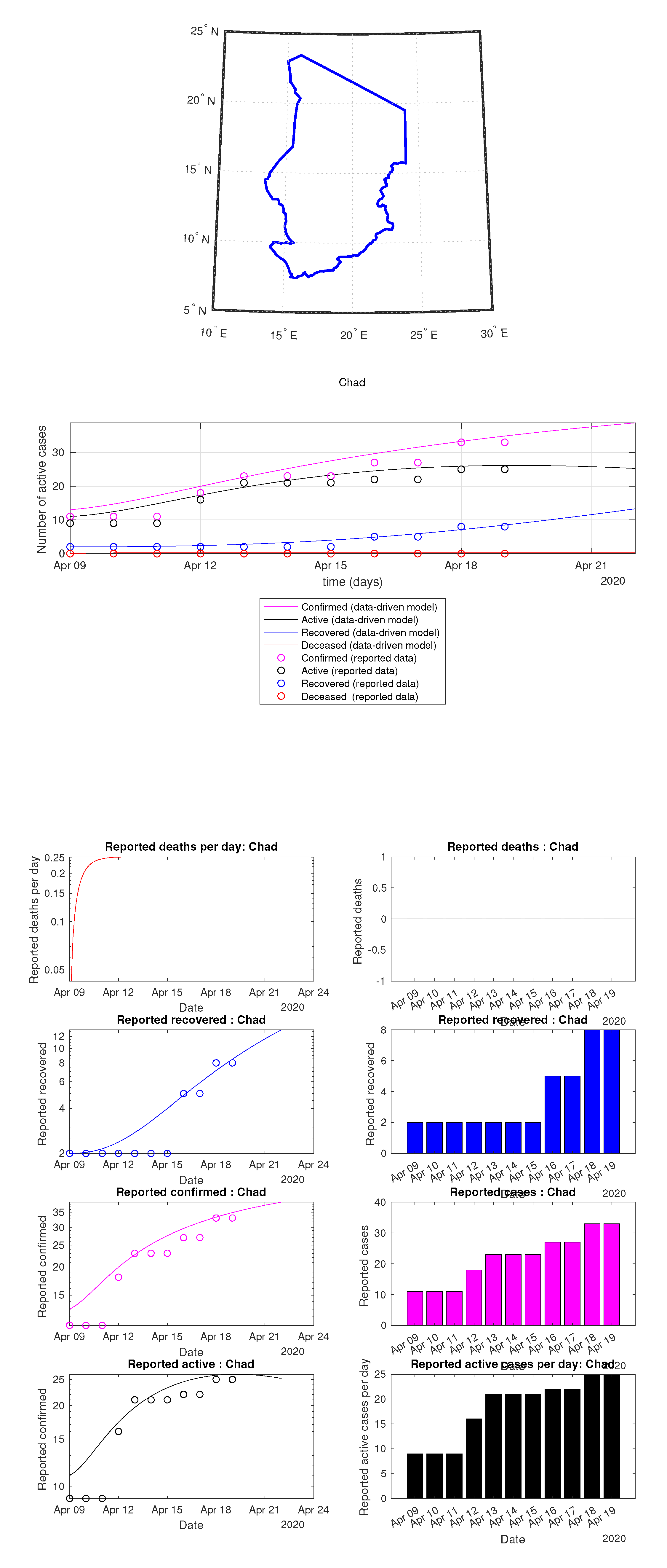
Figure 57.
Chad: data vs. model.
Figure 57.
Chad: data vs. model.
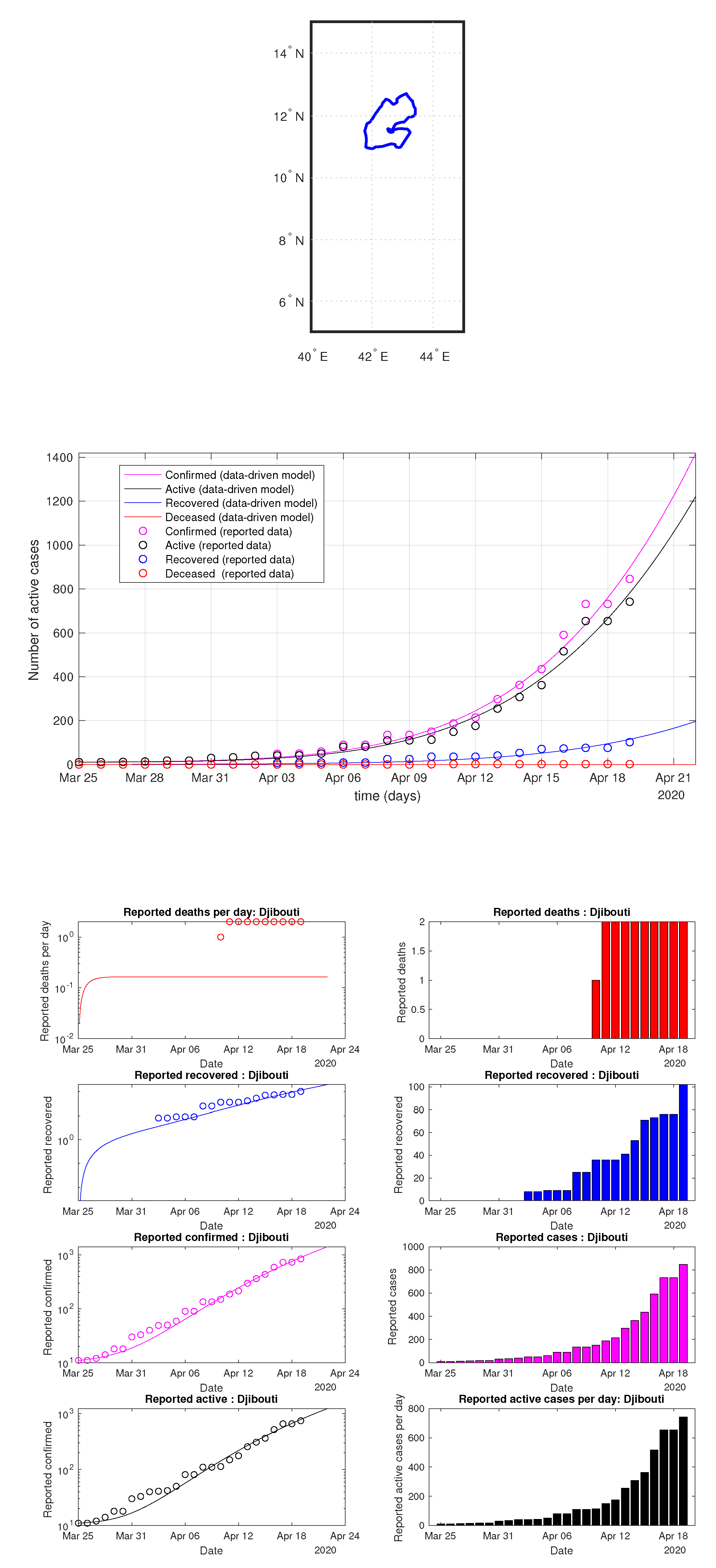
Figure 58.
Djibouti: data vs. model.
Figure 58.
Djibouti: data vs. model.
Figure 59.
Egypt: data vs. model.
Figure 59.
Egypt: data vs. model.
Figure 60.
Eritrea: data vs. model.
Figure 60.
Eritrea: data vs. model.
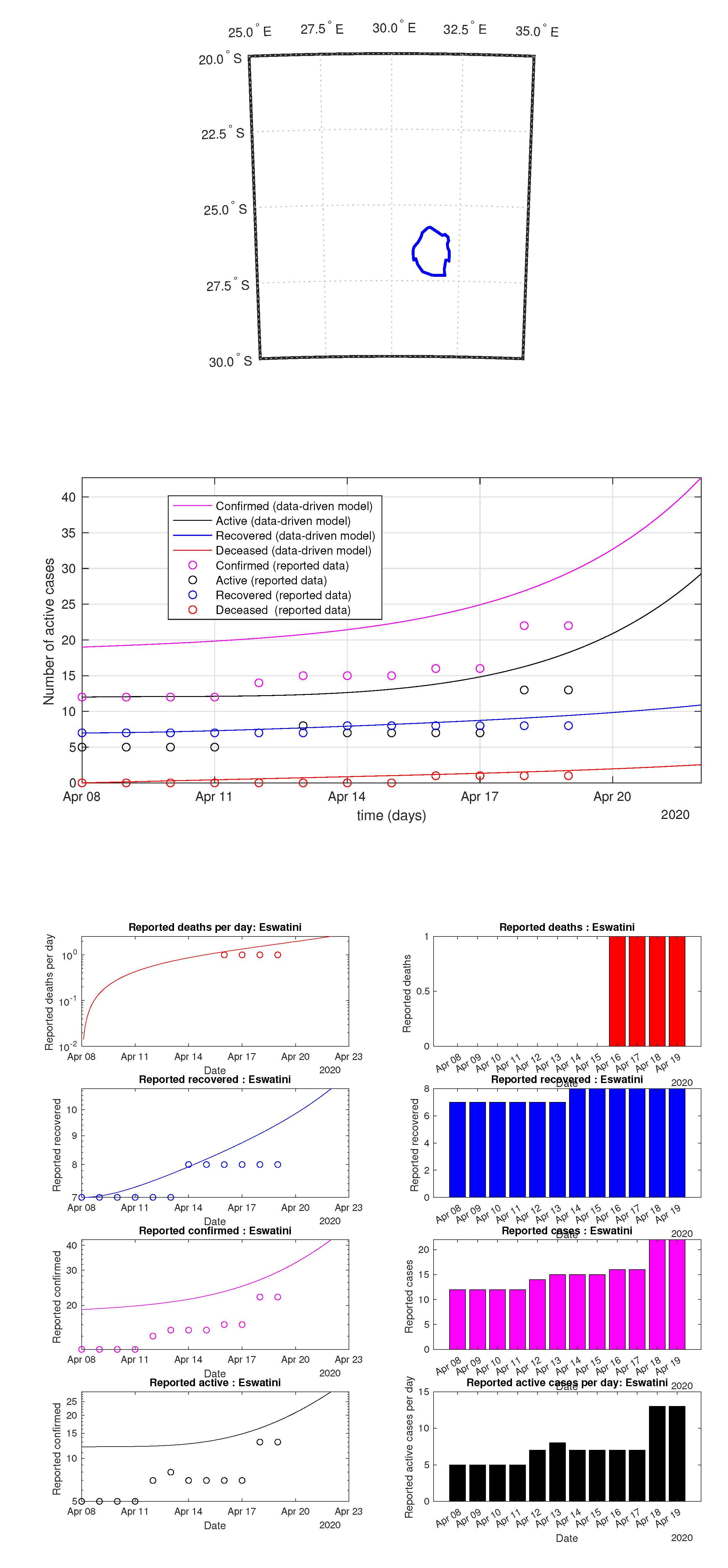
Figure 61.
Eswatini: data vs. model.
Figure 61.
Eswatini: data vs. model.
Figure 62.
Ethiopia: data vs. model.
Figure 62.
Ethiopia: data vs. model.
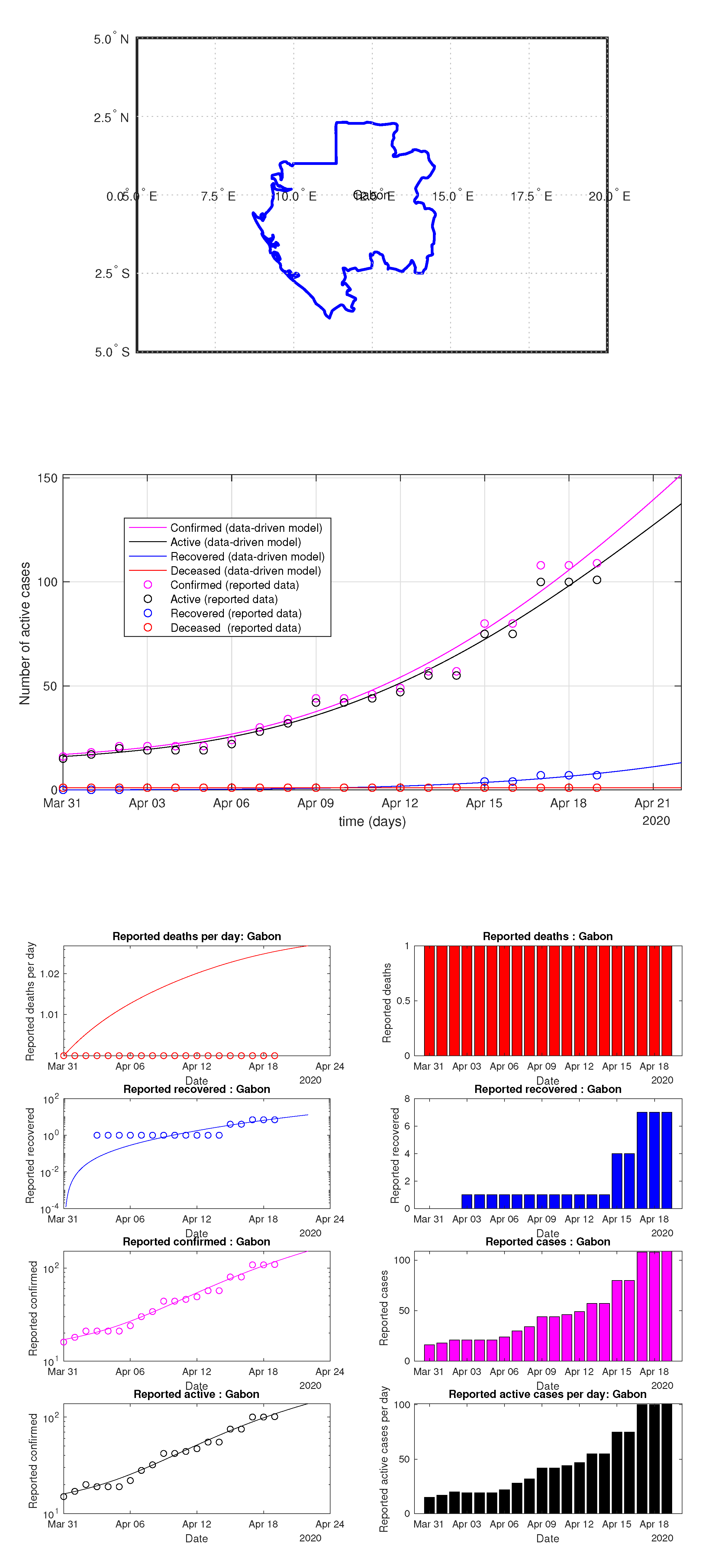
Figure 63.
Gabon: data vs. model.
Figure 63.
Gabon: data vs. model.
Figure 64.
Ghana: data vs. model.
Figure 64.
Ghana: data vs. model.
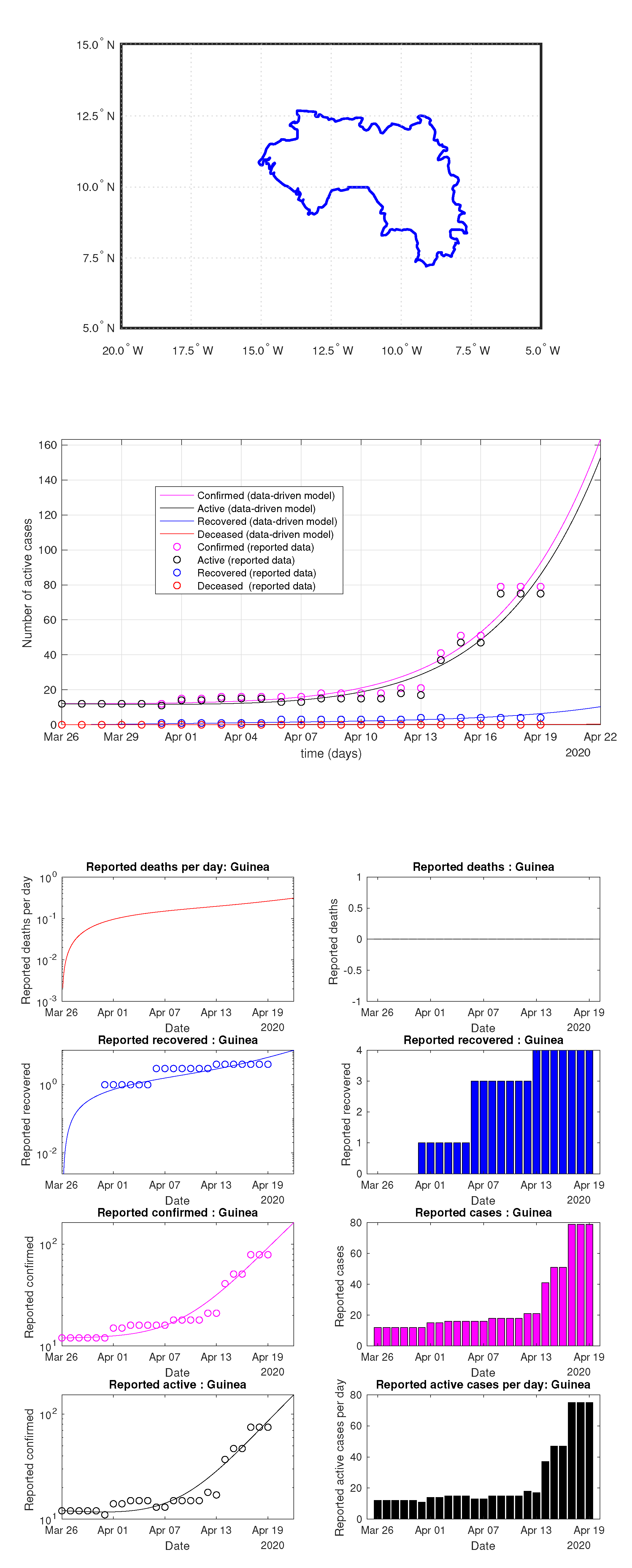
Figure 65.
Guinea: data vs. model.
Figure 65.
Guinea: data vs. model.
Figure 66.
Guinea-Bissau: data vs. model.
Figure 66.
Guinea-Bissau: data vs. model.
Figure 67.
Kenya: data vs. model.
Figure 67.
Kenya: data vs. model.
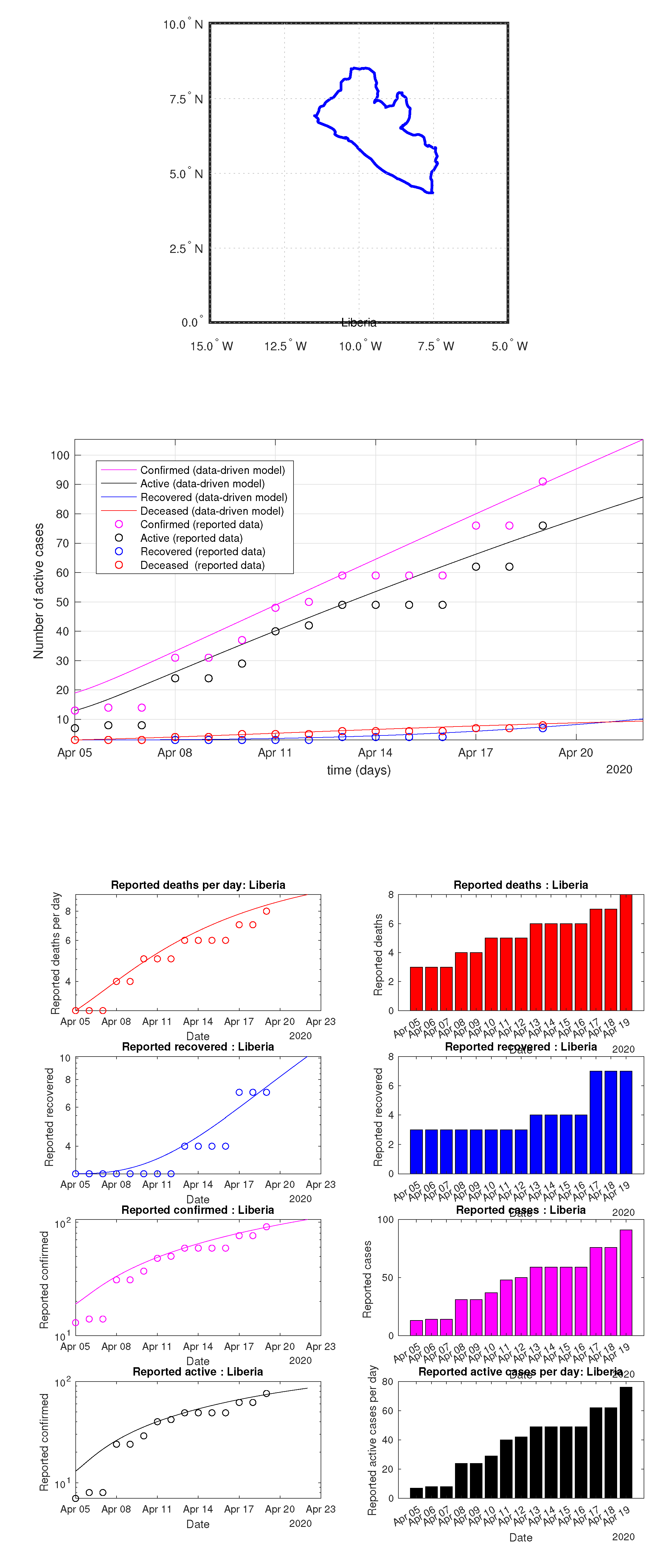
Figure 68.
Liberia: data vs. model.
Figure 68.
Liberia: data vs. model.
Figure 69.
Libya: data vs. model.
Figure 69.
Libya: data vs. model.
Figure 70.
Madagascar: data vs. model.
Figure 70.
Madagascar: data vs. model.
Figure 71.
Malawi: data vs. model.
Figure 71.
Malawi: data vs. model.
Figure 72.
Mali: data vs. model.
Figure 72.
Mali: data vs. model.
Figure 73.
Mauritania: data vs. model.
Figure 73.
Mauritania: data vs. model.
Figure 74.
Mauritius: data vs. model.
Figure 74.
Mauritius: data vs. model.
Figure 75.
Morocco: data vs. model.
Figure 75.
Morocco: data vs. model.
Figure 76.
Mozambique: data vs. model.
Figure 76.
Mozambique: data vs. model.
Figure 77.
Namibia: data vs. model.
Figure 77.
Namibia: data vs. model.
Figure 78.
Niger: data vs. model.
Figure 78.
Niger: data vs. model.
Figure 79.
Nigeria: data vs. model.
Figure 79.
Nigeria: data vs. model.
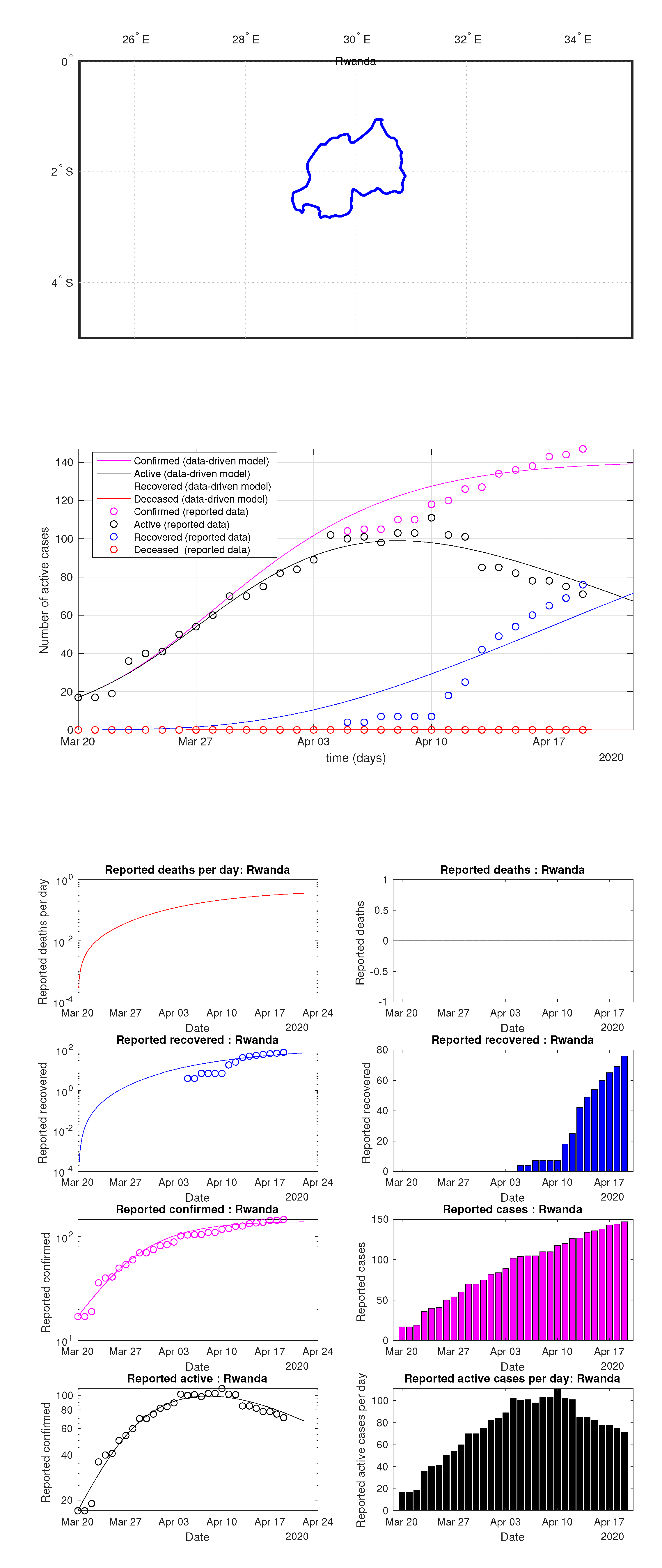
Figure 80.
Rwanda: data vs. model.
Figure 80.
Rwanda: data vs. model.
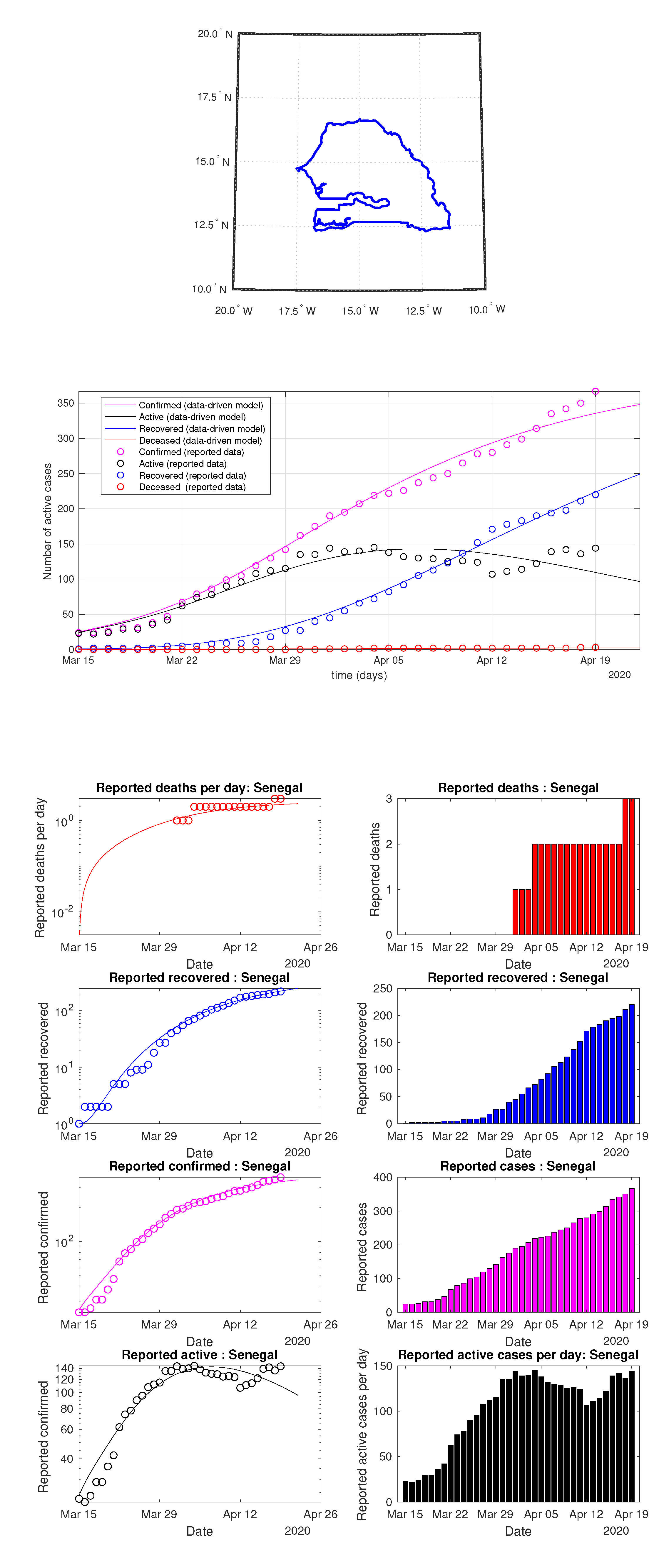
Figure 81.
Senegal: data vs. model.
Figure 81.
Senegal: data vs. model.
Figure 82.
Seychelles: data vs. model.
Figure 82.
Seychelles: data vs. model.
Figure 83.
Somalia: data vs. model.
Figure 83.
Somalia: data vs. model.
Figure 84.
SouthAfrica: data vs. model.
Figure 84.
SouthAfrica: data vs. model.
Figure 85.
Sudan: data vs. model.
Figure 85.
Sudan: data vs. model.
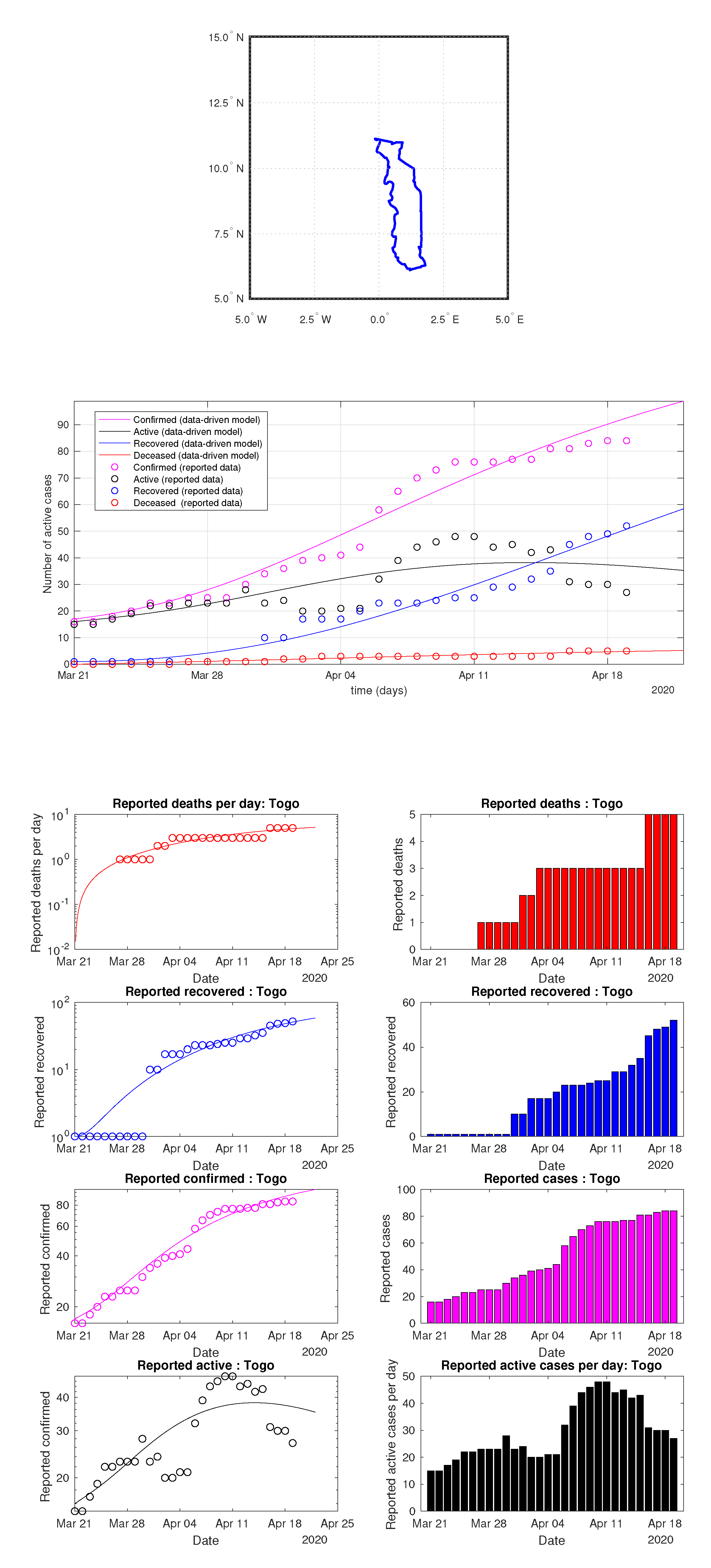
Figure 86.
Togo: data vs. model.
Figure 86.
Togo: data vs. model.
Figure 87.
Tunisia: data vs. model.
Figure 87.
Tunisia: data vs. model.
Figure 88.
Uganda: data vs. model.
Figure 88.
Uganda: data vs. model.
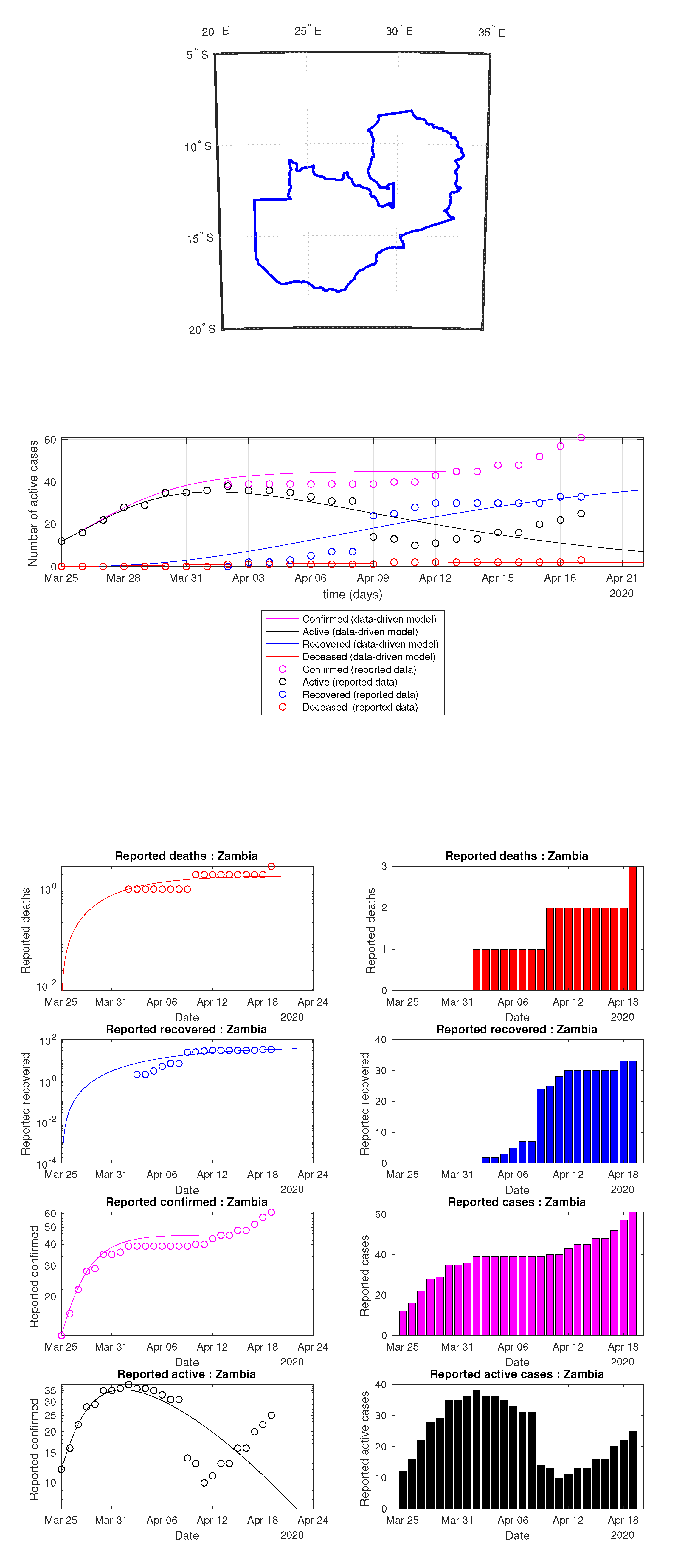
Figure 89.
Zambia: data vs. model.
Figure 89.
Zambia: data vs. model.
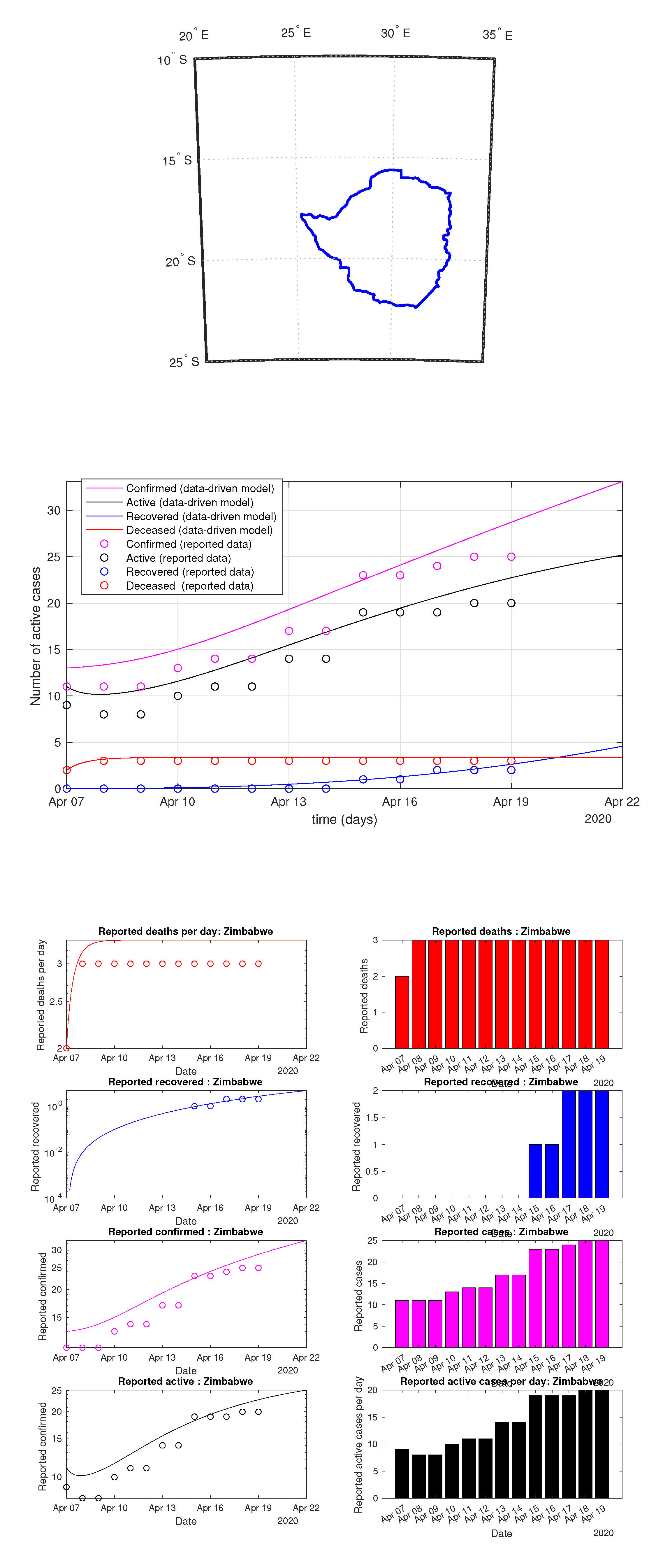
Figure 90.
Zimbabwe: data vs. model.
Figure 90.
Zimbabwe: data vs. model.
Table 1.
Key features of the data-driven MFTG model.
Table 1.
Key features of the data-driven MFTG model.
| Feature | SIR | SEIR | SEIRD | SEIR-Spatial | SEIR -Age Structured | MFTG |
|---|
| locality | no | no | no | no | no | yes |
| city | no | no | no | no | no | yes |
| sector per city | no | no | no | no | no | yes |
| position | no | no | no | yes | no | yes |
| infection status | 3 states | 4 | 5 | 4 | 4 | 17 |
| age | no | no | no | no | yes | yes |
| gender | no | no | no | no | no | yes |
| height | no | no | no | no | no | yes |
| health | no | no | no | no | no | yes |
| family size | no | no | no | no | no | yes |
| economic status | no | no | no | no | no | yes |
| testing strategy | no | no | no | no | no | yes |
| decision-making | no | no | no | no | no | yes |
| untested positive | no | no | no | no | no | yes |
| data-driven | no | no | no | no | no | yes |
Table 2.
Heterogenous data sources.
Table 2.
Heterogenous data sources.
| Data | Sources |
|---|
| International connectivity per country | Flightradar24 [34] |
| Age structure per country | [35] |
| COVID-19 data set | [10,11,12,13,36] |
| Local mobility | Google Community |
| | Mobility Reports [37] |
| Country-specific hospital capacity data | World Bank Group [38] |
| Geographical map | OpenStreet map |
| Economic policy | IMF |
Table 3.
Some notations used the proposed model.
Table 3.
Some notations used the proposed model.
| Symbols | Meaning |
|---|
| l | locality |
| country, city, area |
| temperature field |
| migration between countries |
| migration between cities |
| local mobility between areas of a city |
| z | age variable |
| initial age distribution |
| testing capacity per week |
| testing strategy at l |
| pre-existing health condition, |
| | gender, height, family size, economic wealth |
| position of an individual agent |
| v | velocity of an individual agent |
| s | individual epidemiological states |
| subpopulation size at locality l |
| u | meeting/activity strategy |
| m | mean-field |
| f | Drift |
| interaction kernel |
| physical distancing of 2 m |
| e | economic wealth |
Table 4.
List 1 of figures and illustrations.
Table 4.
List 1 of figures and illustrations.
Table 5.
List 2 of figures and illustrations. data of active, recovered, deceased (in circle or bar) vs. model of active, recovered, deceased over time. Tracking the number of active cases. Predictive analytics for the next couple days.
Table 5.
List 2 of figures and illustrations. data of active, recovered, deceased (in circle or bar) vs. model of active, recovered, deceased over time. Tracking the number of active cases. Predictive analytics for the next couple days.
Table 6.
List 3 of figures and illustrations. data of active, recovered, deceased (in circle or bar) vs. model of active, recovered, deceased over time. Tracking the number of active cases. Predictive analytics for the next couple days.
Table 6.
List 3 of figures and illustrations. data of active, recovered, deceased (in circle or bar) vs. model of active, recovered, deceased over time. Tracking the number of active cases. Predictive analytics for the next couple days.
Table 7.
List 4 of figures and illustrations. data of active, recovered, deceased (in circle or bar) vs. model of active, recovered, deceased over time. Tracking the number of active cases. Predictive analytics for the next couple days.
Table 7.
List 4 of figures and illustrations. data of active, recovered, deceased (in circle or bar) vs. model of active, recovered, deceased over time. Tracking the number of active cases. Predictive analytics for the next couple days.


