Article

Give and Let Give: Alternative Mechanisms Based on Voluntary Contributions †

Department of Management, Technology and Economics, ETH Zurich, 8092 Zurich, Switzerland
The author is indebted to Heinrich Nax for in-depth discussions and for introducing him to relevant literature.
Games 2019, 10(2), 21; https://doi.org/10.3390/g10020021
Submission received: 28 February 2019 / Revised: 24 April 2019 / Accepted: 30 April 2019 / Published: 7 May 2019
(This article belongs to the Special Issue Social Norm and Risk Attitudes)

Abstract

:
We propose a new family of mechanisms, whereby players may give more or less directly to one another. A cornerstone case is the regular linear public goods mechanism (LPGM), where all contribute into a single common group account, the total amount of which is then distributed equally among players. We show that with sufficiently (yet not necessarily fully) pro-social preferences, the social optimum can be reached in Nash equilibrium in all social dilemma situations described by our mechanisms (including the LPGM). In addition, for a given heterogeneity of pro-social preferences, we help to identify which specific mechanisms perform best in terms of incentivizing giving. Our results are therefore relevant from two vantage points. One, they provide proper rational choice benchmarks based on Nash equilibrium under the assumption of other-regarding preferences. Two, they provide arguments in favor of re-structuring many collective action problems currently implemented as LPGMs when it is feasible to gain some information concerning who has concern for whom.

1. Introduction

Humans often depend on mechanisms facilitating mutual help, support, or charity. Public goods mechanisms (PGMs), as introduced by Marwell and Ames [1], are archetypal schemes of this kind: they are among the most widely studied in experimental economics, and many real-world situations are modeled as such: the public good is produced only if individuals overcome selfish and strategic incentives to free-ride.1 However, given narrowly selfish preferences (and without additional components such as punishment, reputation, etc.), this is standardly not the case, and the outcomes are inefficient.2 In the present note, where we focus on linear PGMs (LPGMs), we show that this prediction can change quite drastically if we assume that individuals have other-regarding preferences.3 Specifically, the assumption is that players have heterogeneous “concerns” for the material well-being of others, rather than being narrowly self-interested.4 Based on the levels and distributions of these pro-social concerns, as well as on the rate of return of the underlying LPGM, we show that equilibrium contributions in an LPGM often have a bang-bang structure. That is, total contributions are quite generically either zero despite many players being substantially pro-social or they amount to full contributions even if players are not perfectly altruistic. Intermediate contributions are oftentimes inconsistent with the Nash equilibrium.5
Our results on LPGMs are embedded in a more general approach where we apply our techniques to an entire family of new voluntary contribution mechanisms, which we shall refer to as “giving circles mechanisms” (GCMs).6 GCMs differ with respect to how many players are directly affected by one’s decision to contribute. More specifically, we assume that players are arranged on a circle and can donate to their m ( m { 1 , , n } ) next neighbors in, say, clockwise direction; if m = n , we recover the LPGM; if m = 1 , the GCM constitutes a simple closed loop of contribution opportunities that are made from player to player. For intermediate values of m, players’ contributions reach some, but not all of the players along the circle.7 See Figure 1 for an illustration.
Our analysis reveals that all games induced by GCMs (i.e., for any m) share the above-mentioned bang-bang equilibrium structure. However, which specific candidate of this family of mechanisms will lead to full contributions and thus potentially to a social optimum is a difficult question, as it depends not only on the basic constituents of the game (i.e., rate of return, population size), but also on the detailed psychology of the players in terms of how others are affected by their concerns. In the present note, we show that for suitably “localized” concerns, fundamental corollaries can nevertheless be drawn in quite general terms, thereby unveiling conditions for the existence of simple welfare-superior alternatives to the LPGM based on GCMs. We also point out situations in which such mechanisms may be fruitful and thus hope to contribute toward finding better mechanisms to support voluntary contributions in collective action problems.

2. An Interpolating Family of Mechanisms

We start by presenting the family of GCMs and show in what sense they interpolate between two existing mechanisms in the literature; the LPGM at one extreme and the “dictator loop” at the other.8 We then introduce social preferences and explore their consequences in terms of resulting Nash equilibria.

2.1. Giving Circle Mechanisms of Range m

We consider a set of n players. Each player i ( i = 1 , , n ) chooses a contribution π i [ 0 , 1 ] . Her/his final material payoff is:
x i = 1 π i + p m j = i m i 1 π j , ( m { 1 , , n } ) ,
where negative indices are determined modulo n, that is whenever j = i m 0 , we replace j by j = j + n . In essence, what Mechanism (1) does is that every player obtains p m × the payment from each of her/his m predecessors, where p > 0 is the multiplier of redistribution (“rate of return”). Equivalently, every player’s payment is equally distributed over her/his m successors. We therefore refer to Equation (1) as a GCM with range m, or simply “m-GCM”. To relate with the Introduction, note that for m = 1 , we obtain a mechanism where each player makes a payment to her/his immediate neighbor (“simple giving circle”). If m = n , the resulting mechanism is the LPGM. For varying m, the scheme thus interpolates gradually between the simple giving circle (1-GCM) and the LPGM (n-GCM); see again Figure 1.

2.2. Utility Functions

We assume that any player i’s utility function is of the Cobb–Douglas form,
u i ( π 1 , , π n ) : = k = 1 n x k ( π 1 , , π n ) c k ( i ) ,
where the x j 0 denote material payoffs for each player j and { c k ( i ) } k = 1 , , n are player i’s concerns for others. Specifically, c i ( i ) is the concern that player i has for himself/herself, and k i c k ( i ) is the total concern that player i has for the other players. We require c k ( i ) 0 for all i and k and k = 1 n c k ( i ) = 1 for all i. Moreover, we define 0 0 = 1 throughout this paper.

2.3. Pure-Strategy Nash Equilibria

In combination with the utility functions (2), any m-GCM naturally induces a game that allows for a Nash equilibrium analysis. The next theorem presents the aforementioned bang-bang structure in the case that players are either all sufficiently selfish or all sufficiently altruistic (we do not consider mixed cases).
Theorem 1.
For any m { 1 , , n } , the game induced by an m-GCM admits the following Nash equilibria.
  • If c i ( i ) p m k = i + 1 i + m c k ( i ) for all i, then
    ( π 1 * , , π n * ) = ( 0 , , 0 )
    is a Nash equilibrium. In the case of strict inequalities, this is the unique (pure strategy9) strict equilibrium. For m = n , it is also the unique pure strategy equilibrium.
  • If c i ( i ) p m k = i + 1 i + m c k ( i ) for all i, then
    ( π 1 * , , π n * ) = ( 1 , , 1 )
    is a Nash equilibrium. In the case of strict inequalities, this is the unique (pure strategy) strict equilibrium. For m = n , it is also the unique pure strategy equilibrium.
The proof of Theorem 1 is found in the Appendix A. We mention that for m < n , the uniqueness results do not extend to all pure strategy equilibria for technical reasons due to the particular form of the utility functions (2). In that case, a subset of players may “coincidentally coordinate” in a manner that renders them mutually indifferent, resulting in alternative (albeit unstable) equilibria. Two clarifying examples are given in the Appendix B. To avoid such pathological cases as well as an overly technical discussion, we therefore focus on strict equilibria as regards uniqueness. Alternatively, under the additional assumptions made for the applications in the next section, it turns out that non-strict equilibria in fact disappear altogether.

2.4. Interpolation

In order to better understand how m-GCMs interpolate between the LPGM and the dictator loop in terms of equilibrium behavior, the transition from m = n 1 to m = n requires special attention: only the case m = n guarantees that each player receives a non-zero material payoff. Specifically, for m = n 1 , the condition for the full-giving equilibrium is
c i ( i ) p n 1 k i c k ( i ) = p n 1 1 c i ( i ) c i ( i ) p p + n 1 for all i ,
while for m = n , it is
c i ( i ) p n .
In absence of a social dilemma, i.e., if n p , Condition (4) is trivially satisfied because in that case, full-giving is a (weakly) dominant strategy even for narrowly selfish players; in contrast to the case m = n 1 . If 1 p n , the cases m = n 1 and m = n are still rather different. In the latter case, every player (almost) gets back any amount she/he decides to pay, letting full-giving, despite no longer being dominant, remain an equilibrium even for quite moderate pro-social concerns. By contrast, if m = n 1 , this is not true, and a given player needs substantially more concern for others for non-zero payments to results in equilibrium. If 1 p n , the two mechanisms become strategically comparable, as then, a player’s contribution to herself/himself in the LPGM, p n π i , becomes very small: Conditions (3) and (4) are then very similar. It is thus in this scenario that m-GCMs interpolate “monotonically” between the simple giving circle (1-GCM) and the LPGM (n-GCM). Table 1 summarizes the basic properties of m-GCMs.

3. Choice of an Optimal Mechanism

In this section, we use the Nash equilibrium predictions established in the previous section in order to identify those mechanisms that are conducive to implement the social optimum. To do so, we must first make explicit some assumptions regarding how players’ concerns are distributed.

3.1. Localized Bracketing

Players’s preferences are assumed to differ in terms of “bracketing”, that is in terms of how deep along the circle their concerns affect other players: are only immediate successors relevant (the ones one gives to directly) or do successors’ successors, etc., matter as well? We restrict our attention to situations where players have localized concerns, meaning that they care about the final material payoff of some of their successors, but not necessarily for those that are more distant along the loop. Specifically, we assume that players can be arranged so that anyone’s concerns are “l-localized” ( l n ), meaning that c i + l ( i ) 0 for at least one i and c k ( i ) = 0 for k { i , i + 1 , , i + l } for all i. For example, if l = 1 , each player only has non-zero concern for herself/himself and her/his immediate successor. As mentioned above, the following uniqueness claim makes no assumption on the strictness of equilibria and is a corollary of the proof of Theorem 1.
Corollary 1.
Suppose all concerns are l-localized for some l m . Then, the following holds:
  • If c i ( i ) > p m k = i + 1 i + m c k ( i ) for all i, then
    ( π 1 * , , π n * ) = ( 0 , , 0 )
    is the unique pure strategy Nash equilibrium.
  • If c i ( i ) < p m k = i + 1 i + m c k ( i ) for all i, then
    ( π 1 * , , π n * ) = ( 1 , , 1 )
    is the unique pure strategy Nash equilibrium.

3.2. Optimal Mechanisms

For the given bracketing assumptions, we intend to identify which m-GCM can optimally stimulate spending, i.e., the full-giving equilibrium. While we suspect a general answer to this question to be rather complex as it depends on the detailed structure of the concern distribution, several partial answers can be given. To do so, we focus on l-localized concerns and situations as described in Theorem 1 and Corollary 1, where we can use the explicit full-giving condition,
c i ( i ) < p m k = i + 1 i + m c k ( i ) for all i ,
to identify values of m that support the social optimum for p > 1 (for p < 1 , read “pessimum” instead). We shall consider a mechanism to be more suitable to implement full-giving if the corresponding equilibrium condition is less demanding on the pro-sociality of concerns. Specifically, for l m < n , Condition (5) simplifies to
c i ( i ) < p m 1 c i ( i ) c i ( i ) < p p + m for all i ,
which, using the monotonicity of p p p + m , implies a first domination principle.
Observation 1.
The l-GCM imposes less strict conditions on full-giving than the m-GCM for all m with l < m < n .
The case m = n (LPGM) is different because the sum on the right-hand side of (5) then includes the concern for self, c i ( i ) , which need not be zero. Using Condition (4), it follows that the l-GCM outperforms the LPGM if and only if
p n < p p + l
from which a second observation is an immediate consequence.
Observation 2.
The l-GCM imposes less strict conditions on full-giving than the LPGM if and only if p + l < n .
In other words, the l-GCM is more “likely” to dominate the LPGM in terms of full-giving, the smaller the multiplier of redistribution, the more localized the bracketing, or the more players are involved. For example, if l = 1 (very narrow bracketing), it suffices that p < n 1 .10 Conversely, for l = n 1 , the LPGM dominates in terms of full-giving for all p > 1 and in terms of zero giving for all p < 1 ; it is thus more socially desirable for all p in case of very broad bracketing.
Observations 1 and 2 contain quite general information as regards the sub-optimality of m-GCMs with m > l . As regards the case m l , we content ourselves with the example of l-localized and uniform concerns, that is for fixed l < n and all i, let
c k ( i ) = 1 c i ( i ) l if k = i + 1 , , i + l , 0 else .
It then holds that for
p m k = i + 1 i + m c k ( i ) = p l ( 1 c i ( i ) ) for all m l < n .
Thus, for l-localized and uniform concerns, all m-GCMs with m l impose the very same condition for full-giving.

4. Implications and Conclusions

In the present note, we have proposed a new family of mechanisms based on voluntary contributions that comprises different constellations of how giving and receiving are arranged. The pre-existent literature has equated interactions based on voluntary contributions with only one of the extremes of this family, which is the mechanism where all players pay into a common group account, the total amount of which is then multiplied and divided equally amongst all players.11 That mechanism, which we have labeled as LPGM here, but is often referred to as the voluntary contributions mechanism (cf. Footnote 6), suffers from major shortcomings. For instance, it has been shown not to lead to sustained provision of the public goods in numerous experimental studies [3,4]. What is more, it suffers from several instabilities for various types of preferences [9,10]. Our analysis suggests that several promising alternative voluntary contributions mechanisms exist that deserve further scrutiny.
We find that, depending on whether social preferences exist and how they are distributed, GCMs other than the LPGM may be better suited to achieve the social optimum. Specifically, we identify conditions under which certain m-GCMs (m determines how many of n total players each individual player’s giving reaches) dominate others in terms of incentivizing full-giving. Specifically, if intense and personalized concerns are prevalent and can be organized in a loop, so that they display a certain degree of localization, we find that too large values of m < n are dominated by smaller m, and the same is true of the LPGM ( m = n ) unless the multiplier of redistribution is very large or only very few players are involved. As a consequence, for large populations, instead of considering one single LPGM, it may be more advisable to consider either smaller groups of disjoint LPGMs (e.g., in the spirit of so-called “climate clubs” [11]) or to use an appropriate alternative m-GCM as suggested by our results.12 This is a particularly practical question as large LPGMs are omnipresent in international cooperation, e.g., in the most prominent Bretton Woods institutions such as the IMF and the World Bank ( n = 189 each), the UN ( n = 193 ), or the EU ( n = 27 / 28 ).
Despite the potential advantages of m-GCMs, there are of course also some limitations. Importantly, an arrangement of players, such that all their concerns are suitably localized, may not exist. Even if it exists, it requires that the mechanism designer has access to reliable information concerning the distribution of social preferences. Ordering players in a giving circle without such knowledge can result in the chain of concerns breaking along the loop, which in turn can have detrimental consequences for overall giving. In view of that, LPGMs can be a less risky option in situations of limited information regarding the distribution of concerns. Note, however, that there are many situations where it is natural to assume that such information is indeed readily available, e.g., citizens having predominantly concern for their neighbors, countries for their neighboring countries, people for people similar to them, etc. Even where the availability of such information is not immediate, future research could reveal additional mechanisms that help to reveal individual concerns truthfully.
In sum, our central message is that even if a mechanism designer cannot go beyond relying on voluntary contributions, she/he may do substantially better than implementing an LPGM, namely by means of an alternative GCM, provided that social preferences are distributed in certain ways and that she/he has sufficient information concerning this distribution.

Funding

This research received no external funding.

Conflicts of Interest

The author declares no conflict of interest.

Appendix A. Proofs

Proof of Theorem 1.
We start by computing the partial derivative
π i u i = π i k = 1 n x k c k ( i ) = k = 1 n x k c k ( i ) k = 1 n π i x k c k ( i ) x k c k ( i ) = u i k = 1 n c k ( i ) x k π i x k = u i p m k = i + 1 i + m c k ( i ) x k c i ( i ) x i .
Item 1. To show that ( π 1 * , , π n * ) = ( 0 , , 0 ) is an equilibrium, observe that
π i u i ( 0 , , 0 , π i , 0 , , 0 ) = u i ( 0 , , 0 , π i , 0 , , 0 ) p m k = i + 1 i + m δ m n c k ( i ) 1 + p m π i ( 1 δ m n p m ) c i ( i ) 1 ( 1 δ m n p n ) π i = k = i + 1 i + m δ m n 1 + p m π i c k ( i ) ( 1 ( 1 δ m n p n ) π i ) c i ( i ) a s d f l k j a l d f k j a l d s j × p m k = i + 1 i + m δ m n c k ( i ) 1 + p m π i ( 1 δ m n p m ) c i ( i ) 1 ( 1 δ m n p n ) π i
where δ m n : = 1 if m = n and δ m n : = 0 else (Kronecker delta). Using 1 + p m π i 1 ( 1 δ m n p n ) π i 0 and p m k = i + 1 i + m c k ( i ) c i ( i ) 0 , we readily obtain
π i u i ( 0 , , 0 , π i , 0 , , 0 ) u i ( 0 , , 0 , π i , 0 , , 0 ) 1 + p m π i p m k = i + 1 i + m c k ( i ) c i ( i ) 0 for all π i [ 0 , 1 ] ,
(including the possibility that π i u i ( 0 , , 0 , π i = 1 , 0 , , 0 ) = ) from which it follows that ( π 1 * , , π n * ) = ( 0 , , 0 ) is an equilibrium.
In the case of strict inequalities, i.e., p m k = i + 1 i + m c k ( i ) c i ( i ) < 0 for all i, note that u i ( 0 , , 0 , π i , 0 , , 0 ) > 0 and, hence, π i u i ( 0 , , 0 , π i , 0 , , 0 ) < 0 with the only potential exception being the single point π i = 1 . As a consequence, π i u i ( 0 , , 0 , π i , 0 , , 0 ) must be strictly decreasing on all of [ 0 , 1 ] , and so, ( π 1 * , , π n * ) = ( 0 , , 0 ) is a strict equilibrium.13
To show uniqueness in the case of strict inequalities, let ( π 1 * , , π n * ) be an arbitrary strict equilibrium and let i be the player whose material payoff in that equilibrium, x i * : = x i ( π 1 * , , π n * ) , is minimal in the sense that x i * x i * for all i. Assuming for a moment the claim
u i ( π 1 * , , π n * ) = k = 1 n ( x k * ) c k ( i ) > 0 ,
it follows from this minimality, using Equation (A1), that
π i u i ( π 1 * , , π n * ) u i ( π 1 * , , π n * ) x i * p m k = i + 1 i + m c k ( i ) c i ( i ) < 0 ,
and hence, π i * = 0 . However, then, the “donors” of player i + 1 can give at most as much as those of player i ; in the formulas
x i + 1 * x i * = π i + 1 * p m π i m * + 1 + p m π i * = π i + 1 * p m π i m * 0 .
That is, x i + 1 * is also minimal, implying π i + 1 * = 0 . Proceeding inductively along the entire giving circle yields the uniqueness of the zero-giving equilibrium.
To show Inequality (A4), suppose that u i ( π 1 * , , π n * ) = 0 (minimal utility). If player i unilaterally changes her/his payment to deviate from π i * , then her/his utility either increases, which contradicts ( π 1 * , , π n * ) being an equilibrium, or stays minimal, which contradicts ( π 1 * , , π n * ) being a strict equilibrium.
Finally, if m = n , then Inequality (A4) holds regardless of whether or not the equilibrium ( π 1 * , , π n * ) is strict, since for arbitrary i, x i * = 0 is impossible by Definition 1.
Item 2. The proof is analogous to that of Item 1, and we follow the latter in a practically verbatim manner to clarify where and how it differs from that of Item 2. In order to prove that ( π 1 * , , π n * ) = ( 1 , , 1 ) is an equilibrium, observe that
π i u i ( 1 , , 1 , π i , 1 , , 1 ) = u i ( 1 , , 1 , π i , 1 , , 1 ) × p m k = i + 1 i + m δ m n c k ( i ) p m ( ( m 1 ) + π i ) ( 1 δ m n p n ) c i ( i ) 1 ( 1 p n δ m n ) π i + p m ( m δ m n ) .
Using 1 ( 1 p n δ m n ) π i + p m ( m δ m n ) p m ( ( m 1 ) + π i ) 0 and p m k = i + 1 i + m c k ( i ) c i ( i ) 0 , we readily obtain
π i u i ( 1 , , 1 , π i , 1 , , 1 ) u i ( 1 , , 1 , π i , 1 , , 1 ) p m ( ( m 1 ) + π i ) p m k = i + 1 i + m c k ( i ) c i ( i ) 0 for all π i [ 0 , 1 ] ,
(including the possibility that π i u i ( 1 , , 1 , π i = 0 , 1 , , 1 ) = ) from which it follows that ( π 1 * , , π n * ) = ( 1 , , 1 ) is an equilibrium.
In the case of strict inequalities, i.e., p m k = i + 1 i + m c k ( i ) c i ( i ) > 0 for all i, note that u i ( 1 , , 1 , π i , 1 , , 1 ) > 0 and, hence, π i u i ( 1 , , 1 , π i , 1 , , 1 ) > 0 with the only potential exception being the single point π i = 0 . As a consequence, π u i ( 0 , , 0 , π i , 0 , , 0 ) must be strictly increasing on all of [ 0 , 1 ] , and so, ( π 1 * , , π n * ) = ( 1 , , 1 ) is a strict equilibrium.14
To show the uniqueness in the case of strict inequalities, let ( π 1 * , , π n * ) be an arbitrary strict equilibrium and let i be the player whose material payoff in that equilibrium, x i * , is maximal in the sense that x i * x i * for all i. Using Inequality (A4), for which the above proof is still valid under the assumptions of Item 2, it follows from this maximality that (cf. Equation (A1))
u i π i ( π 1 * , , π n * ) u i ( π 1 * , , π n * ) x i p m k = i + 1 i + m c k ( i ) c i ( i ) > 0 ,
and hence, π i * = 1 . However, then, the “donors” of player i + 1 must give at least as much as those of player i ; in the formulas (cf. Equation (A5)): x i + 1 * x i * 1 π i + 1 * + p m 1 π i m * 0 . Hence, x i + 1 * is also maximal, implying π i + 1 * = 1 . Proceeding inductively along the entire giving circle yields the uniqueness of the full-giving equilibrium. □
Proof of Corollary 1.
Since concerns are l-localized with l m , any player i can make the material payoff of all players for which she/he has concern (including herself/himself) simultaneously non-zero. That is to say, she/he can always pick π i such that u i ( π 1 , , π n ) > 0 regardless of what the other players’ payments are. As a consequence, Inequality (A4) holds, and so, uniqueness follows just like in the proof of Theorem 1. □

Appendix B. “Coincidental Coordination”

As mentioned after Theorem 1, our uniqueness results do not carry over to all pure strategy equilibria in the case m < n . Indeed, it can then occur that players who are unable to change each other’s material payoffs coincidentally make extremal payments that make each other indifferent, thereby violating Inequality (A4).
Example A1.
Consider a 1-GCM with n = 4 players and multiplier of redistribution p = 1 . Let Players 1 and 3 be perfectly selfish, c 1 ( 1 ) = c 3 ( 3 ) = 1 , and Players 2 and 4 be moderately altruistic, c 4 ( 2 ) = c 2 ( 4 ) = ε > 0 and c 2 ( 2 ) = c 4 ( 4 ) = 1 ε > 0 (it follows that all other concerns are zero). Then, the conditions of Theorem 1, Item 1, are satisfied with strict inequalities, and it is readily verified that
( π 1 * , π 2 * , π 3 * , π 4 * ) = ( 0 , 1 , 0 , 1 )
is a (non-strict) Nash equilibrium. It is however very unstable in the following sense: if Player 2, who is indifferent with regards to her/his own payment in this equilibrium, deviates ever so slightly from π 2 * = 1 , then Player 4 is no longer indifferent, and her/his (now unique) best reply jumps to π 4 = 0 . But then, Player 2’s best reply is also unique and equals π 2 = 0 , resulting in the zero-giving equilibrium described in Theorem 1.15 By symmetry, the same argument can of course be made with the roles of Players 2 and 4 interchanged.
It is readily seen that the “coincidental coordination” of indifferent players and the induced equilibrium instability in the above example is a feature of all such alternative pure strategy equilibria. Of course, generally, there may be more than two players that render each other indifferent in equilibrium. We close with an analogue to Example A1 if instead the conditions of Theorem 1, Item 2, are met.
Example A2.
Consider again a 1-GCM with n = 4 players and multiplier of redistribution p = 1 . Let Players 1 and 3 be perfectly altruistic with respect to their immediate successor, c 2 ( 1 ) = c 4 ( 3 ) = 1 , and Players 2 and 4 satisfy c 1 ( 2 ) = c 3 ( 4 ) = ε > 0 and c 3 ( 2 ) = c 1 ( 4 ) = 1 ε > 0 (it follows that all other concerns are zero). Then, the conditions of Theorem 1, Item 2, are satisfied with strict inequalities, and it is readily verified that
( π 1 * , π 2 * , π 3 * , π 4 * ) = ( 1 , 0 , 1 , 0 )
is a (non-strict) Nash equilibrium.

References

  1. Marwell, G.; Ames, R.E. Experiments on the Provision of Public Goods. I. Resources, Interest, Group Size, and the Free-Rider Problem. Am. J. Sociol. 1979, 84, 1335–1360. [Google Scholar] [CrossRef]
  2. Isaac, M.R.; McCue, K.F.; Plott, C.R. Public goods provision in an experimental environment. J. Public Econ. 1985, 26, 51–74. [Google Scholar] [CrossRef] [Green Version]
  3. Ledyard, J.O. Public Goods: A Survey of Experimental Research. In Handbook of Experimental Economics; Kagel, J.H., Roth, A.E., Eds.; Princeton University Press: Princeton, NJ, USA, 1995; pp. 111–194. [Google Scholar]
  4. Chaudhuri, A. Sustaining cooperation in laboratory public goods experiments: a selective survey of the literature. Exp. Econ. 2011, 14, 47–83. [Google Scholar] [CrossRef]
  5. Groves, T.; Ledyard, J.O. Optimal Allocation of Public Goods: A Solution to the “Free Rider” Problem. Econometrica 1977, 45, 783–809. [Google Scholar] [CrossRef]
  6. Healy, P.J.; Jain, R. Generalized Groves–Ledyard mechanisms. Games Econ. Behav. 2017, 101, 204–217. [Google Scholar] [CrossRef]
  7. Fehr-Duda, H.; Fehr, E. Sustainability: Game human nature. Nat. News 2016, 530, 413. [Google Scholar] [CrossRef] [PubMed]
  8. Grech, P.; Nax, H.H. Nash Equilibria of dictator games: A new perspective. Preprint 2018. [Google Scholar] [CrossRef]
  9. Saijo, T. The Instability of the Voluntary Contribution Mechanism; Working Papers SDES-2014-3; Kochi University of Technology, School of Economics and Management: Kochi, Japan, 2014. [Google Scholar]
  10. Feng, J.; Saijo, T.; Shen, J.; Qin, X. Instability in the voluntary contribution mechanism with a quasi-linear payoff function: An experimental analysis. J. Behav. Exp. Econ. 2018, 72, 67–77. [Google Scholar] [CrossRef]
  11. Nordhaus, W. Climate Clubs: Overcoming Free-Riding in International Climate Policy. Am. Econ. Rev. 2015, 105, 1339–1370. [Google Scholar] [CrossRef]
  12. Isaac, R.M.; Walker, J.M. Group Size Effects in Public Goods Provision: The Voluntary Contributions Mechanism. Q. J. Econ. 1988, 103, 179–199. [Google Scholar] [CrossRef]
1
Marwell and Ames [1] used the terminology of “voluntary contribution mechanism” instead; see also Footnote 6 below. For other related treatments of public goods games, see [2], as well as [3,4] for reviews.
2
Groves and Ledyard [5] identified special environments under which the free-riding problem can be overcome; see also [6] for an extension.
3
Broadly, one categorizes PGMs by linear, minimum, and maximum aggregation technologies, that is dependent on whether the resulting public good is determined by the average contribution, the lowest individual contribution, or the highest individual contribution. The different PGMs model different situations depending on whether it is the total effort or one of the extreme contributions that determines the societal benefit. The highest individual contribution, for example, may be relevant when members of a society (separately, yet bound by common destiny) attempt to solve a problem, while the total contribution may be more relevant for a pollution abatement situation (linear aggregation).
4
Indeed, the fact that many humans typically have other-regarding preferences is widely accepted [7] and often used to explain experimental LPGM data [3,4]. More surprising is the fact that there seems to be no analysis of the resulting consequences in terms of Nash equilibria of the game induced by the LPGM once this assumption is made.
5
The same effect, applying a similar reasoning to (“interactive”) dictator games, was found in [8]. The proof strategy given here is however different as we do not assume a “representative agent” as in that paper.
6
In the scholarly literature, LPGMs (and with some abuse of terminology, also linear “public goods games”) are often labeled as “voluntary contributions mechanisms” with linear aggregation technology. Given that all GCMs are also based on voluntary contributions, we avoid this alternative nomenclature here in order to prevent confusion.
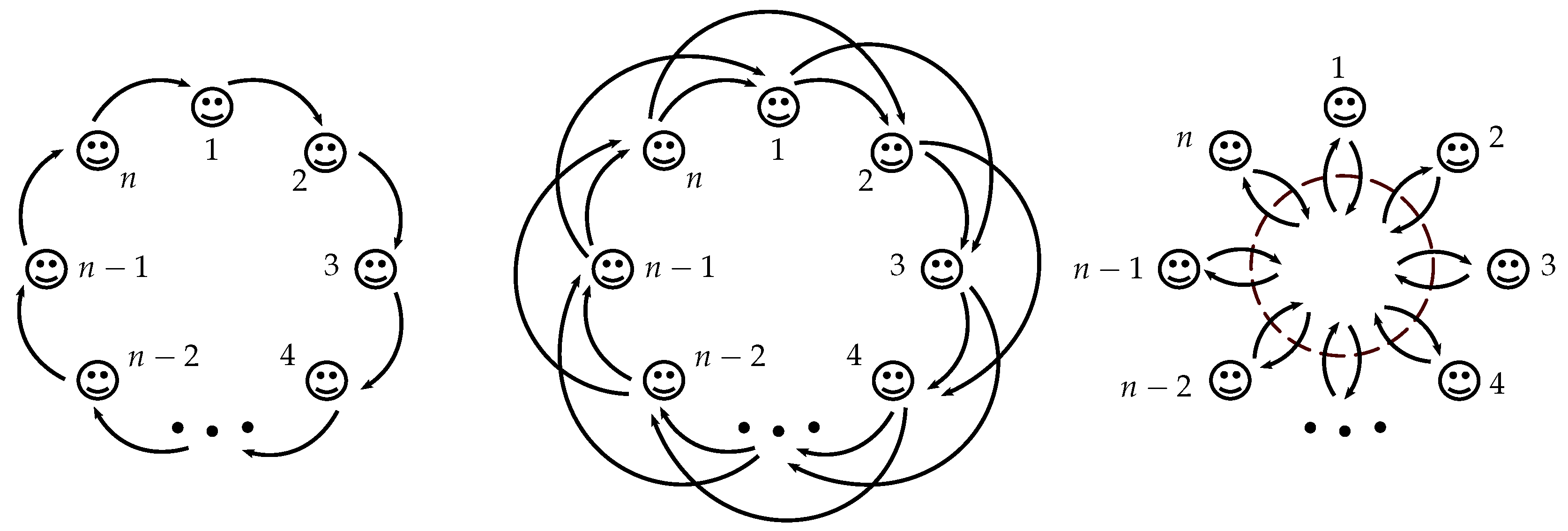
7
To illustrate, imagine the two extreme mechanisms (with m = 1 and m = n ) were to be implemented in a church congregation. While the LPGM is akin to an alms basket being collected, potentially multiplied, and then shared equally amongst all, a GCM with m = 1 involves envelopes of offerings (potentially multiplied and) being passed from each person to their next neighbor, say on the right.
8
Dictator loops have recently been found to occur in many dictator game experiments [8].
9
While we are exclusively focusing on pure strategies in the present paper, recall that strict Nash equilibria are necessarily pure strategies. The qualifier in brackets is thus, strictly speaking, superfluous.
10
Recall that for n p , full-giving is a (weakly) dominant strategy for the LPGM even for narrowly selfish preferences.
11
The other extreme is somewhat more “incognito” in the existing literature, cf. Footnote 8.
12
See [12] for a related experimental analysis of the group size effect in public goods provisions.
13
In fact, π i u i ( 0 , , π i = 1 , , 0 ) < 0 since for c i ( i ) = 0 , it holds that u i ( 0 , , π i = 1 , , 0 ) > 0 , for 0 < c ( i ) < 1 , it holds that u i ( 0 , , π i = 1 , , 0 ) > 0 if m = n ; by Equation (A2), we have π i u i ( 0 , , 0 , 0 , π i = 1 , 0 , , 0 ) = if m < n ; and finally, for c i ( i ) = 1 , we have π i u i ( 0 , , 0 , 0 , π i = 1 , 0 , , 0 ) = 1 .
14
A similar reasoning to the one in Footnote 13 shows that in fact, π i u i ( 1 , , π i = 0 , , 1 ) > 0 .
15
We caution the reader that, while related, this stability notion is not identical to trembling-hand perfection, as the latter relies on totally-mixed strategies.
Figure 1. An interpolating family of mechanisms. Left: simple giving circle (1-GCM). Center: 2-GCM. Right: linear public goods mechanism (LPGM); the LPGM is identical to the n-GCM as each player’s contribution is then equally distributed over all her/his successors including herself/himself.
Games 10 00021 g001
Table 1. Characteristics of the game induced by the m-GCM.
Initial Individual Endowment1
Individual outcome m = n m < n
maximal 1 + ( n 1 ) p n 1 + p
minimal p n 0
Collective outcome p 1 p 1
maximal p n n
minimaln p n
Equilibrium thresholdszero giving c i ( i ) p m k = i + 1 i + m c k ( i ) i
full-giving c i ( i ) p m k = i + 1 i + m c k ( i ) i

