1. Introduction
Distractions can be loosely defined as events that take away the attention from what you are supposed to be doing. In the context of a brain–computer interface (BCI), these are unwanted, and the current practice in this field is to avoid them through the careful design of experiments. The work presented here is part of a larger electroencephalography (EEG)-based project and in continuation of our latest papers [
1,
2], with the goal of building an extendible hierarchical taxonomy aimed at categorizing distractions and the effects thereof. In addition, this paper is an extension of work originally presented in [
3], which is also in continuation of the aforementioned papers.
BCI research and development has been predominantly focused on the speed and accuracy of the BCI application but has been wanting in usability, such as the environment in which it is being used. In fact, many BCI applications and experiments were and are still being performed in laboratory settings with unrealistic conditions, where the subject sits in a sound-attenuated room without any distractions [
4,
5]. A number of research papers, such as [
6,
7], focus on real-world contexts, however, they were either using medical-grade equipment [
8] and/or focusing on auditory event-related potentials (ERPs) [
9].
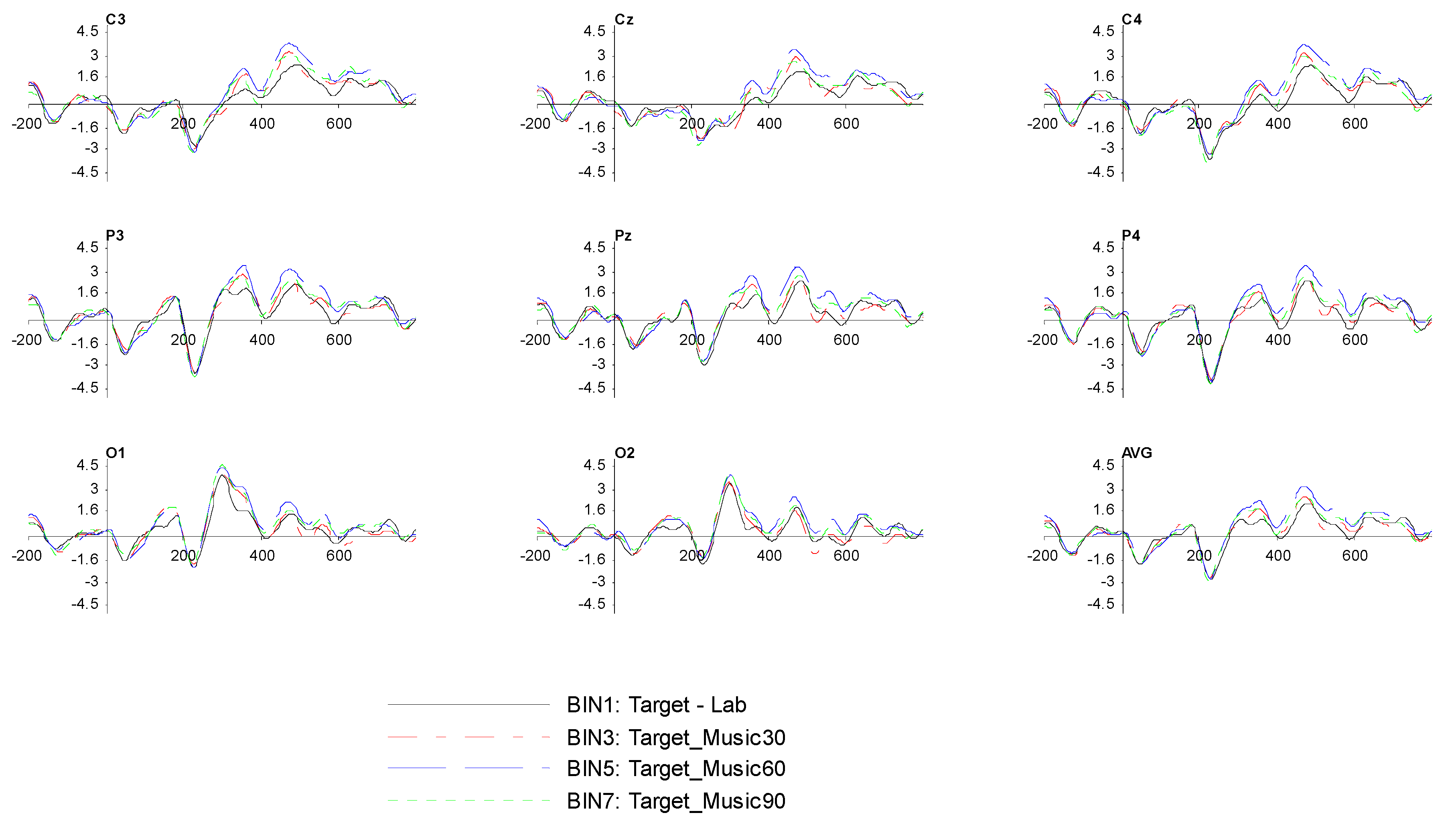
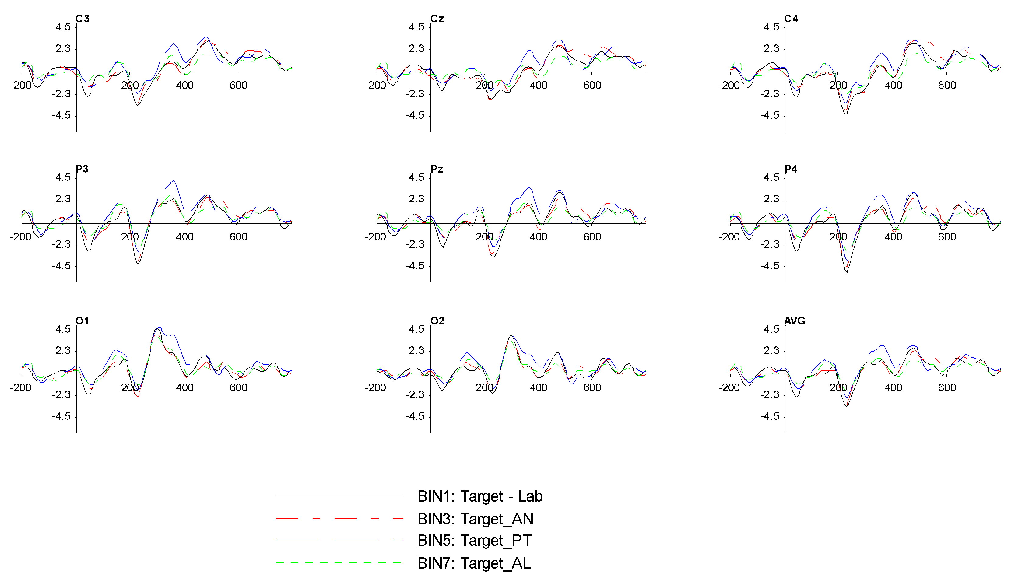
Our goal is to analyze the effect that distractions have on the signal characteristics of a P300 component while using the P300 speller paradigm alongside the continuous development of taxonomy. In this paper, we specifically analyze the effect that auditory distractions, explicitly that of music at 30% (
M30), music at 60% (
M60), music at 90% (
M90), ambient noise (
AN), passive talking (
PT), and active listening (
AL), have on the signal of a visual P300 speller in terms of accuracy, amplitude, latency, user preference, signal morphology, and overall signal quality. This work includes data and comparisons from our previous papers [
2,
3]. In addition, our research makes use of non-invasive BCI on the basis of EEG. The contribution of this work is to provide researchers with a ground reference taxonomy that enables them to compare and extrapolate EEG signal detection results between different distractions and to be able to predict and assess the effects of a particular distraction and/or an environment containing those distractions.
The requirement for this work was derived from the need to broaden the utilization of this technology for both subjects with neuromuscular disabilities and healthy individuals, by providing a solution which is assessed outside lab conditions, i.e., in noisy environments, and based on low-cost equipment. In the absence of comprehensive studies on the effect that distractions have in relation to the P300 performance, i.e., for accuracy and signal characteristics, an evident necessity for this study was present. Our null hypothesis, based on previous research [
2,
3], is that this type of distraction does not show any statistically significant effect on accuracy, task performance, amplitude, latency, or signal morphology.
In this work, we report a study where eight to ten healthy subjects used a Farwell and Donchin P300 speller paradigm in conjunction with the xDAWN algorithm [
10] while utilizing low-cost off-the-shelf equipment. The subjects were asked to communicate five alphanumeric characters, referred to as symbols, in the different settings mentioned above. The main aim of this study was to systematically examine the usability of a P300 speller BCI, in terms of the effect that the independent variables, i.e., each distraction, has on the dependent variables when compared to the dependent variable lab condition (LC). Empirical experiments were performed to measure how environmental factors, such as the aforementioned settings, affect the signal characteristics and performance of the P300 component. This work forms part of a larger EEG-based project where we have instituted [
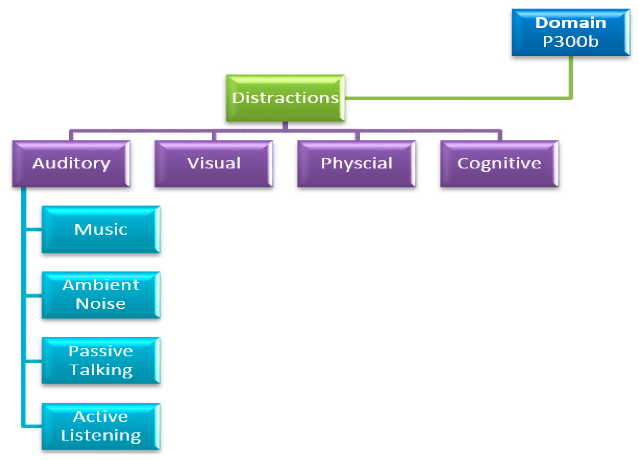
2] a set of distinctive categories for distractions in conjunction with the continuous development of a hierarchical taxonomy, as portrayed in
Figure 1.
This paper is structured as follows: the methodology, which includes the research background, equipment, participants, and experimental procedures, is described in
Section 2. The offline and online ERP results and the user preferences are presented in
Section 3. The conclusion is given in
Section 4.
2. Methodology
The following segment/s of the methodology are from the authors’ previous work, as referenced above, and are adopted and outlined in the current paper for readers’ convenience.
2.1. Research Background
ERPs are slow voltage fluctuations or electrical potential shifts recorded from the nervous system. These are time locked to perceptual events following a presentation of a stimulus, being cognitive, sensor, or motor stimuli. The simplest paradigm for eliciting an ERP is by focusing attention on the target stimuli (occur infrequently) embedded randomly in an array of non-targets (occur frequently). The methodology used derives from the oddball paradigm first used in ERPs by Squires, Squires, and Hillyard [
11], where the subject is asked to distinguish between a common stimulus (non-target) and a rare stimulus (target). The target stimuli elicit one of the most renowned ERP components, known as P300, which is an exogenous and spontaneous component and was first described by Sutton [
12]. The name is derived from the fact that it is a positive wave that appears approximately 300 ms after the target stimulus. Unless otherwise noted in this paper, the term P300 (P3) will always refer to the P300b (P3b), which is elicited by task-relevant stimuli in the centro-parietal area of the brain.
There were several studies with the aim of improving the performance of P300-BCI systems. For instance, Qu et al. [
13] focused on a new P300 speller paradigm based on three-dimensional (3-D) stereo visual stimuli, while Gu et al.’s [
14] primary focus was within the single character P300 paradigm, i.e., they evaluated the posterior probability of each character in the stimuli set to be the target. Even though improving the performance and execution of the application is an important aspect, this should not come at the expense of the environment in which it is used, such as that of a real-world context. In fact, current practice in the field is either to avoid distractions through the careful design of experiments or environments or to filter out these distractions (and the effects thereof). As such, there has not been a rigorous classification of such distractions within a range of intensities, nor is there currently a mapping between distraction type and the effects caused.
For instance, [
6] focused on assessing how background noise and interface color contrast affect user performance, while [
7] focused on the experimental validation of a readout circuit, which is a wearable low-power design with long-term power autonomy device aimed at the acquisition of extremely weak biopotentials in real-world applications. Additionally, [
8] introduced methods for benchmarking the suitability of new EEG technologies by performing an auditory oddball task using three different medical-grade EEG systems, while seated and walking on a treadmill. Moreover, [
9] evaluated the ERP and single-trial characteristics of a three-class auditory oddball paradigm recorded in outdoor scenarios while peddling on a fixed bike or freely biking around.
2.2. Hardware
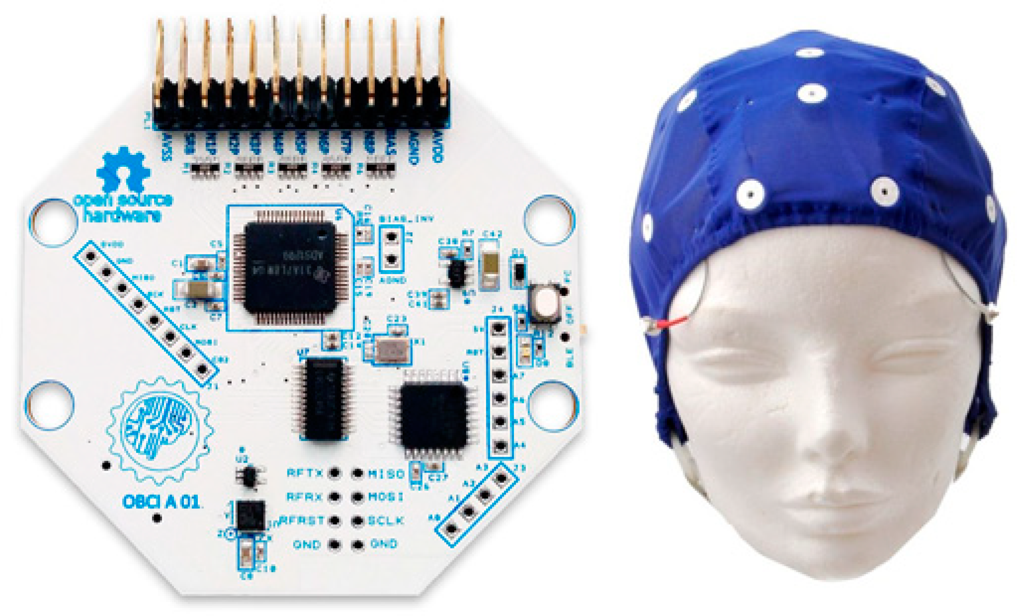
Our work utilized the OpenBCI 32-bit board (dubbed Cyton) in conjunction with the Electro-Cap, as depicted in
Figure 2 which, in the context of EEG experiments, is based on the international 10/20 system for electrode placement on the scalp.
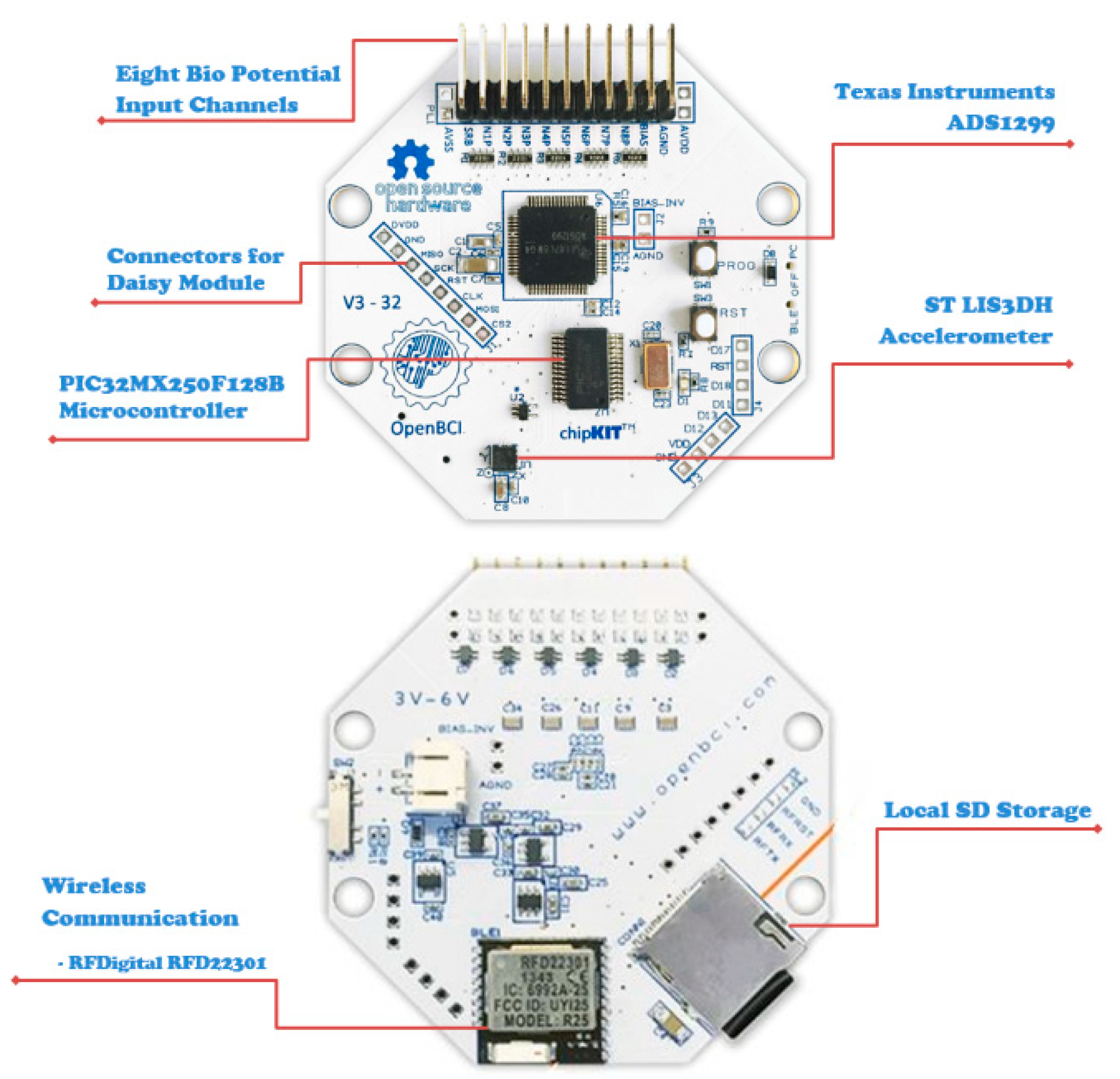
The PIC32MX250F128B microcontroller found on the Cyton board has a 32-bit processor with a 50 MHz ceiling and 32 KB of memory storage, while being Arduino compatible. It also encompasses an ADS1299 IC, which is an eight-channel, 24-bit, simultaneous sampling delta-sigma, analog-to-digital converter used for biopotential measurements, developed by Texas Instruments. In addition, it has a built-in low-cost microcontroller, the RFDuino RFD22301, for wireless communication, which communicates with the provided and pre-programmed USB dongle. In our previous paper [
15], the reader can obtain a more in-depth elucidation of the Cyton board and its built-in hardware components, which are depicted in
Figure 3 for the reader’s convenience.
In addition, our work utilized the Electro-Cap, which is made of fabric, explicitly that of elastic spandex. The electrodes, which are directly attached to the fabric, are made of pure tin and are considered as wet electrodes. This implies that an electrolyte gel must be applied to the electrodes to have effective scalp contact. Otherwise, we could end up with impedance instability.
To output our six diverse distractions, i.e., music at 30%, music at 60%, music at 90%, ambient noise, passive talking, and active listening, we used a pair of Creative Labs SBS 15 speakers, which can output a nominal root mean square (RMS) power of 5 Watts for each speaker, which have a frequency response of 90 Hz–20,000 Hz and a 90dB signal-to-noise ratio (SNR).
2.3. Participants
For the first session, which included the independent variables LC, M30, M60, and M90, we enrolled N = 10 healthy subjects, of which seven were males and three were females. They were aged between 29 and 38, with a mean age of 33.8, and their participation was on a voluntary basis.
For the second session, which included the independent variables AN, PT, and AL, we enrolled N = 8 healthy subjects, of which six were males and two were females. They were aged between 29 and 38, with a mean age of 33.8, and their participation was on a voluntary basis. The native language of seven of the eight subjects was Maltese, while the native language for the final subject was English.
However, all subjects in both sessions were au fait with the English language and were conversant with the alphanumeric symbols portrayed in the P300 speller application. In addition, all subjects had previous experience with P300-BCI experiments.
Another subject aided in the groundwork and initial testing for the configuration of our equipment, and in the development of the methodology, however, he/she did not partake in the official experiments and hence his/her data are not included in the results.
For both sessions, the subjects were instructed to avoid consuming any food or drinks, apart from water, for one hour prior to the start of the experiment. Moreover, the total averaged reported sleep the night before the experiment was 467.5 min (29.05).
2.4. Data Acquisition
We set the sampling rate and sampling precision for the EEG signal at the hardware’s ceiling of 250 Hz and 24 bits, respectively. The raw data were stored anonymously in OpenVIBE. ov format, however, for offline analysis, this was converted to a comma-separated value (CSV) format and imported into MATLAB. The stored raw data included the readings of eight EEG electrodes, namely, C3, Cz, C4, P3, Pz, P4, O1, and O2, which were placed in accordance with the International 10–20 System.
Since the spatial amplitude dispersal of the P300 component is symmetric around Cz and its electrical potential is maximal in the midline region (Cz, Pz) [
16], we opted to use the aforementioned electrodes. In addition, and in view of the fact that, in general, an earlobe or a mastoid reference generates a robust P300 response, we opted for a referential montage, with the reference electrode placed on the left earlobe (A1) and the ground electrode placed on the right ear lobe (A2).
2.5. P300 Speller and xDAWN
In this work, we utilized the Farewell and Donchin P300 speller in combination with the xDAWN algorithm. This type of methodology is based on visual stimuli which are explained thoroughly below. The subject is presented with thirty-six symbols, i.e., alphanumeric characters, which were positioned in a six by six grid, dubbed the spelling grid. The subject is asked to observe the intensification of each row and column, which for one repetition entails the intensification of six rows and six columns in random order. Then, the subject is asked to differentiate between a rare stimulus (target) which generates a spontaneous and exogenous ERP known as the P300 potential and a common stimulus (non-target) which does not generate this component. This is achieved with the subject focusing his/her attention on the desired symbol (target) while ignoring the other symbols (non-target). This implies that there is one target column and one target row, while there are five non-target columns and five non-target rows, for each repetition. The intersection of the row and column targets predicts what symbol is spelt for that repetition. In the simplest terms, the prediction distinguishes between the target, i.e., a row or column stimulus that produces a P300 component, from the non-target, i.e., a row or column stimulus that does not produce a P300 component. Taking into consideration that the peak potential of the P300 component is between 5–10 µV and that this is entrenched and concealed by artefacts and other brain activities, where the typical EEG signal is ±100 µV, this implies that it would be very hard to predict the correct symbol with one repetition. This also leads to a very low signal-to-noise ratio and the most popular and established way to address this issue is for each symbol to be spelt numerous consecutive times, i.e., more than one repetition per symbol, and then the corresponding column and/or row epochs are averaged over a number of repetitions, thus canceling out components unrelated to stimulus onset.
The xDAWN algorithm is a process of spatial filtering that (1) is a dimensional reduction method that produces a subset of pseudo-channels, dubbed output channels, by a linear combination of the original channels and (2) promotes the appealing part of the signal, such as ERPs, with respect to the noise. The process of xDAWN is applied to the data prior to any classification, for instance, linear discriminant analysis (LDA), which was used for this work. From an abstract point of view, the xDAWN algorithm can be divided into (1) a least square estimation of the evoked responses and (2) a generalized Rayleigh quotient to estimate a set of spatial filters that maximize the signal plus noise ratio (SSNR).
The following is adapted from [
10,
17]. Let X ∈ ℝ
S x C be the EEG data that contain ERPs and noise, with
S samples and
C channels. Let A ∈ ℝ
E x C be the matrix of ERP signals, while
E is the number of temporal samples of the ERP (typically,
E is chosen to correspond to 600 ms or 1 s). Let N ∈ ℝ
S x C be the noise matrix which contains normally distributed noise. The ERP position in the data is given by a Toeplitx matrix D ∈ ℝ
E x S. The data model is given by X = D
TA + N. A is estimated by a least square estimate using a matrix inverse (pseudoinverse), as shown in formula (1).
Let W ∈ ℝ
S x F be the pseudo-channels while
F represents the filters for projection. The result is the filtered data matrix X̃ = XW. According to [
10], the optimal filters W can be found by maximizing the SSNR, as given by the generalized Rayleigh quotient:
The optimization problem is solved by combining a QR matrix decomposition (QRD) with a singular value decomposition (SVD). A more thorough explanation is found in [
10].
2.6. Experimental Design
In this work, we had seven manipulated independent within-subjects variables: (a) lab condition, (b) music at 30%, (c) music at 60%, (d) music at 90%, (e) ambient noise, (f) passive talk, and (g) active listening,. Moreover, we had several dependent measures which were classified into three types of dependent variables, i.e., online performance, which comprised the accuracy, offline performance, which consisted of amplitude and latency, and user preference.
2.6.1. Independent Variables
As previously mentioned, we made use of seven manipulated independent within-subjects variables in two different sessions, which are itemized and elucidated below. It is important to remember that all auditory distractions were performed from the same recording, with the same equipment and at the same level of intensity unless noted otherwise.
Lab condition, abbreviated as LC, where the experiments were performed in a sound-attenuated room, without any distractions.
Music at 30% volume, abbreviated as M30, where the volume level was labeled as “low”, i.e., between 20 and 30dB, and simulated background music.
Music at 60% volume, abbreviated as M60, where the volume level was labeled as “medium”, i.e., between 50 and 60dB, and simulated active listening to a movie.
Music at 90% volume, abbreviated as M90, where the volume level was labeled as “high”, i.e., between 80 and 90dB, and simulated disco-level music only, i.e., there was no crowd chatter or other type of noise.
Ambient noise, abbreviated as AN, where we introduced an auditory distraction that simulated ambient noise, including city traffic noise.
Passive talk, abbreviated as PT, where we simulated persons murmuring.
Active listening, abbreviated as AL, where we simulated several persons discussing a particular topic in a clear and audible manner.
The comparison between independent variables was done as follows: LC versus M30, M60, and M90, and LC versus AN, PT, and AL, respectively, for the dependent variables of amplitude and latency. The setting and configuration for all independent variables were outputted from a recorded simulation by the aforementioned speakers, with the volume set at thirty percent (unless otherwise noted), i.e., between 20 and 30 dB, which simulates a real-world context. We opted to use a recording and the same recording for all subjects since we aimed to make the experiments between subjects as similar as possible. Moreover, this made it possible to increase the level of volume equally in every experiment.
2.6.2. Dependent Variables
In this work, there were three types of dependent measures, which can be sub-categorized into four distinct dependent variables:
Online performance comprised accuracy, which is the comparison of the correctly spelled symbols to the planned target symbols, i.e., in our experiments, we had five planned target symbols—BRAIN.
Offline statistics comprised
amplitude and
latency, where (a) the P300 amplitude (μV) is related to the distribution of the subject’s processing resources assigned to the task. It is defined as the voltage difference between the largest positive peak from the baseline within the P300 latency interval and (b) the P300 latency is considered a measure of cognitive processing time, generally between 300–800 ms [
18] poststimulus, i.e., after target stimulus. In the simplest terms, it is the time interval between the onset of the target stimulus and the peak of the wave.
User preference, where two questionnaires were provided to the subjects to ask for their favorite usage condition. This was ranked from four to one, four being the highest and one being the lowest. The objective for these questionnaires was to compare if user preference was directly related to an increase in the accuracy—online performance—or to a heightened increase in the amplitude—offline performance. Moreover, the questionnaire results can easily be compared between subjects to assess the overall preference and/or reluctance in using this technology in environments which contain those distractions.
2.7. Experimental Procedure
An induction session was held for each subject which was intended to re-educate the subjects on the P300 speller paradigm and hardware being used. We also notified the subjects that:
They would be doing the P300 speller experiment in five unique settings for the first session, i.e., (i) the training phase which was performed in lab conditions, i.e., in a sound-attenuated room (ii) LC, (iii) M30, (iv) M60, and (v) M90, and another five unique settings in the second session, i.e., (vi) training phase (same conditions as the first session), (vii) LC, (viii) AN, (ix) PT, and (x) AL, as elucidated in the independent variables.
They would be spelling the symbols “BRAIN” for (1 ii) to (1 v) and for (1 vii) to (1 x), while for (1 i) and (1 vi), i.e., the training phase, they would be spelling fifteen random symbols.
The first experiment was always the training phase in both sessions, i.e., (1 i) and (1 vi) since this was required as training for the system to be able to predict the correct symbols in the subsequent experiments. Then, (1 ii) to (1 v) and (1 vii) to (1 x) were done in a randomized order to circumvent the subjects’ accustomization to that particular distraction. Then, the subjects were asked if they had any queries which were promptly answered at this stage. The subjects were then asked to be seated and relax for a few minutes prior to the start of the experiments. The setup was as follows: (a) the subject was seated facing the display, approximately one meter away, (b) the researcher was situated at the left-hand side of the subject and refrained from making any type of movement or noise throughout. We opted to stay to the side of the subject, since from our experience and subjects’ feedback, they were not comfortable with someone being behind them, (c) the speakers were placed at a 15-degree angle facing the subject and were situated near the monitor, i.e., one meter away from the subject, and (d) the electrode impedance was verified to be less than 5 KΩ. The experiment only started when the subject had no additional questions, was in a comfortable position, and was able to perform the task at hand.
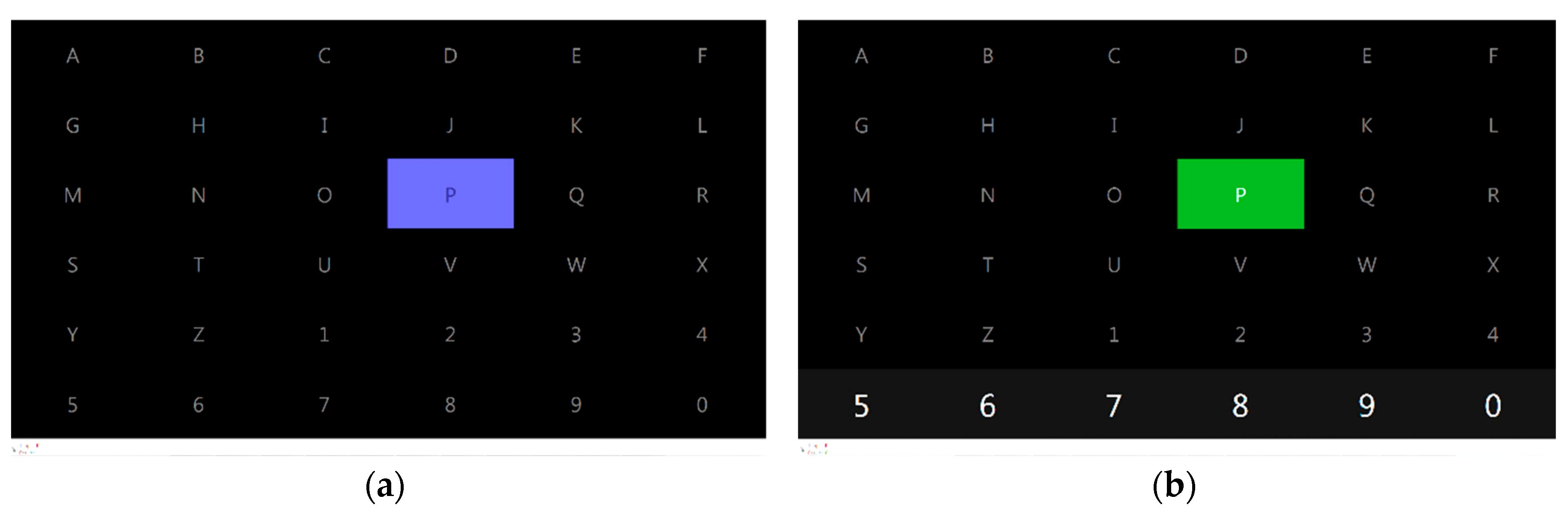
Subsequently, the spelling grid consisting of 36 symbols in a 6 by 6 matrix was presented to the subjects and the target symbol, i.e., the symbol the subject must focus on, was preceded by a cue, i.e., the target symbol was highlighted in blue, as depicted in
Figure 4a. Next, there was a random intensification of 100 ms for each row and column in the matrix and there was an 80 ms delay between two successive intensifications, i.e., after one column and one row was intensified. This implies that we had an interstimulus interval (ISI) of 180 ms. Afterwards, and to predict each symbol, there were fifteen repetitions (i.e., one trial) which consisted of intensifying six rows and six columns for each repetition, and in between each of the groups of six rows and six columns, i.e., one repetition, there was an inter-repetition delay of 100 ms. At the end of trial, i.e., 6 rows by 6 columns by 15 repetitions, the symbol, which was predicted by the system, was presented to the subject by being highlighted with a green cue, as depicted in
Figure 4b. The subject would be aware if the system predicted the correct target symbol. Moreover, in between trials, i.e., in between different symbols, there was a 3000 ms inter-trial period. At the end of each experiment, the subjects were given a short break.
As previously mentioned, the training phase ((1 i) and (1 vi)) was made up of one session that consisted of 15 random symbols by 15 trials each (i.e., 6 rows and 6 columns per trial * 15 trials = 180 flashes per symbol), and this took approximately 10 min. The LC, M30, M60, M90, AN, PT, and AL were made up of one session each and consisted of five specific symbols that made up the word “BRAIN”, and similarly to the training phase, each symbol had 15 trials, with six rows and six columns per trial, i.e., 180 flashes per symbol, and took approximately 6 min for each independent variable.
In total, we had 15 symbols which were spelled in the training phases, and five symbols which were spelled in the other aforementioned independent variables. Hence, due to the matrix disposition, for the training phase, we had 2700 flashes, of which 450 were targets and 2250 were non-targets, and 900 flashes per independent variable, of which 150 were targets and 750 were non-targets. These values are per subject, the data were stored anonymously, and the subjects were referred to as subject x.
2.8. Signal Processing—Online
OpenViBE 2.0.0 was selected as our online system and also took care of the raw signal acquisition. This application is designed for the processing of real-time biosignal data, is a C++-based software platform, and is well known for its graphical language for the design of signal processing chains. It has two main components called the acquisition server, which interfaces with the Cyton board, reads the raw data signal, and produces a uniform signal stream, which is transmitted to the designer, which in turn is composed of several scenarios where we can structure, construct, and execute signal processing chains.
The acquisition server takes care of obtaining the signal from the Cyton board, however, it does not communicate with the board directly, instead, it provides dedicated drivers to perform this task. The sampling rate of the signal was set at 250 Hz, and consisted of eight EEG channels and three auxiliary channels, with the latter channels being used to broadcast data from the accelerometer. In a single buffer and with accepted values being only powers of two, explicitly from 22 to 29, we set the sample count per sent block to 32, which implies how many samples need to be sent per channel. In addition, the Cyton board reply reading timeout was regulated at 5000 ms, while the flushing timeout was adjusted to 500 ms. Although the version of OpenVibe that we used depends on TCP (Transmission Control Protocol) tagging to align the EEG signal with the simulation markers, we had set the drift tolerance to 20 ms. The issue with this setting is that it can introduce signal artefacts and mask other possible faults, such as driver issues. Even though these issues were not encountered in this work, we have decided to discontinue the use of drift tolerance in future experiments, since when TCP tagging was introduced, it made the drift tolerance mechanism redundant. The P300 speller paradigm was managed by the designer, in which there were a number of scenarios that were executed in order, as thoroughly explained below:
The first scenario was the acquisition of the signal and stimuli markers for the training phase. The recordings included the raw EEG and stimuli.
The second scenario entailed the pre-processing of the signal where it trained the spatial filter using the xDAWN algorithm. The subjects’ data recorded in the training session were utilized with the following configuration and modalities. Initially, we chose to eliminate the last three auxiliary channels, which stored the auxiliary data of the accelerometer since the board was firmly placed on the desk and this information was not required. Subsequently, a Butterworth bandpass filter of 1 Hz–20 Hz was applied with an order of 5 and a ripple (dB) of 0.5 to remove the DC offset, the 50 Hz (60 Hz in some countries) electrical interference, and any signal harmonics and unnecessary frequencies which were not beneficial in our experiments. Next, no signal decimation was used since the sampling rate and count per buffer previously used in the acquisition server were not compatible with the actual signal decimation factor due to the Cyton board’s sampling rate of 250 Hz (no available value in the sample count per block was factorable with 250 Hz). However, we still passed the signal through time-based epoching, which generated “epochs” (signal slices) with a duration of 0.25 s and time offset of 0.25 s between epochs (i.e., we created a temporal buffer to collect the data and forward them into blocks). This implies that there was no overlapping of data and that the inputs for the xDAWN spatial filter and the stimulation-based epoching were based on epochs of 0.25 s rather than the whole data. In the simplest terms, we had one point for every 0.25 s of data, which made our signal coarser. Subsequently, we passed the time-based epochs and stimulations to the stimulation-based epoching, which sliced the signal into chunks of the desired length following a stimulation event. This had an epoch duration of 0.6 s (P300 deviation around 0.3 s after the stimuli) and no offset. Lastly, the stimulations, time-based epochs, and the stimulation-based epochs were passed to the xDAWN trainer, which in the simplest terms, trains spatial filters that best highlight ERPs. The xDAWN expression, utilized in OpenVIBE, which has to be maximized, varies marginally from the original xDAWN (Rivet et al., 2009) formula where the numerator includes only the average of the target signals. In addition, the implemented algorithm maximizes the quantity via a generalized eigenvalue decomposition method in which the best spatial filters are given by the eigenvectors corresponding to the largest eigenvalues (Clerc et al., 2016). This scenario created twenty-four coefficients values in sequence (i.e., eight input channels by three output channels) that were used in the following scenario.
The
third scenario carried on the pre-processing of the signal where it trained the classifier, partially with the values from the previous scenario. Once again, the subjects’ raw data, which were recorded in the training session, were utilized with the elimination of the last three aux channels, the omission of signal decimation, and the application of a Butterworth bandpass filter of 1 Hz–20 Hz, identical to the previous scenario. Subsequently, the parameters of the xDAWN spatial filter that were generated in the second scenario, which included the 24 spatial filter coefficients, 8 input channels, and output 3 output channels. This spatial filter generated three output channels from the original eight input channels, where each output channel was a linear combination of the input channels. The output channels were computed by performing the “sum on
i (
Cij *
Ii)”, as shown in formula (3), where
Ii represents the input channel (
n is set to 8),
Oj represents the output channel, and
Cij is the coefficient of the
ith input channel and
jth output channel in the spatial filter matrix.
Subsequently, the outputted signals (i.e., the three output channels) and the stimulations were equivalently and separately passed through stimulation-based epoching for the target and the non-target selection. These had an epoch duration of 0.6 s and no offset. The output, i.e., both epoch signals (target and non-target) were again separately computed with block averaging and passed through a feature aggregator that combined the received input features into a feature vector that was used for the classification. This implies that two separate feature vector streams were outputted; the target and non-target selections. Ultimately, both vector streams and the stimulations were passed through our classifier trainer. We opted to pass all the data through a single classifier trainer, hence the native multiclass strategy was chosen, which used the classifier training algorithm without a pairwise strategy. The algorithm chosen for our classifier was the regular LDA. The output at this stage was a trained classifier with the settings outputted to a file for use in the next scenario.
The fourth scenario consisted of the actual online experiments and was more complex since it was necessary to collect data, pre-process them, classify them, and provide online feedback to the subject. The front-end consisted of displaying the 6 by 6 grid, flashing rows and columns, and give feedback to the subject. The back-end consisted of a number of processes. Primarily, the data were acquired from the subject in real time and, similar to what was done in the previous scenarios, the last three aux channels were eliminated, signal decimation was omitted, a Butterworth bandpass filter of 1 Hz–20 Hz was used, and the parameters of the xDAWN spatial filter that were generated in the second scenario, which included the twenty-four spatial filter coefficients, were used. Subsequently, the output and the stimulations were passed through the stimulation-based epoching, which had an epoch duration of 0.6 s and no offset. This was then averaged and passed through a feature aggregator to produce a feature vector for the classifier. Lastly, the classifier processor classified the incoming feature vectors by using the previously learned classifier (classifier trainer).
The fifth scenario allowed us to replay the experiments by selecting the raw data file and re-process the functions of the fourth scenario.
2.9. Signal Processing—Offline
In the offline analysis, the following procedure was done for each of LC, M30, M60, M90, AN, PT, and AL. The captured raw data were converted from the proprietary OpenVIBE.ov extension to a more commonly used.csv format using a particular scenario designed for this task. The outputs were two files in.csv format which contained the raw data and stimulations, respectively. These were later imported into MATLAB R2014a tables called samples and stims and then converted to arrays. Subsequently, any unnecessary rows and columns in the samples array were removed. These consisted of the first rows which contained the time header, channel names, and sampling rate; the first column, which contained the time(s) and the last three columns, stored the auxiliary data of the accelerometer. Next, we filtered out the stims array to include the target stimulations with the code (33285); non-target stimulations (33286); visual stimulation stop (32780), which was the start of each flash of a row or column; and segment start (32771), which was the start of each trial (12 flashes, 6 rows, and 6 columns made up one trial). Additional data, such as the sampleTime, samplingFreq, and channelNames variables, were extracted from the data and stored in the workspace. Subsequently, we had to perform a signal inversion due to the hardware and driver implementation.
The samples array was later imported into EEGLAB for processing and for offline analysis. The first process was to apply a bandpass filter of 1–20 HZ to eliminate the environmental electrical interference (50 Hz or 60 Hz dependent on the country), to remove any signal harmonics and unnecessary frequencies which were not beneficial in our experiments and to remove the DC offset. Subsequently, we imported the event info (the stimulations—stim array) into EEGLAB with the format {latency, type, duration} in milliseconds.
Next, the imported data were used in ERPLAB, which is an add-on of EEGLAB and is targeted for ERP analysis. Although the dataset in EEGLAB already contained information about all the individual events, we created an eventlist structure in ERPLAB that consolidated this information and made it easier to access and display; it also allowed ERPLAB to add additional information which was not present in the original EEGLAB list of events. Subsequently, we took every event we wanted to average together and assigned them to a specific bin via the binlister. This contained an abstract description of what kinds of event codes go into a particular bin. In our experiments, we used the following criteria: “{33285}{t<50–150>32780}“ for the target and “{33286}{t<50–150>32780}” for the non-target. This implied that it was time locked to the stimulus events 33,285 (target) or 33,286 (non-target) and must have had the event 32,780 that happened 50 to 150 ms after the target/non-target event. If this criterion was met, it was placed in the appropriate bin.
Subsequently, we extracted the bin-based epochs via ERPLAB (not the EEGLAB version) and set the time period from −0.2 s before the stimulus until 0.8 s after the stimulus. We also used baseline correction (pre-stimulus) since we wanted to subtract the average pre-stimulus voltage from each epoch of data. Next, we passed all channel epoch data through a moving window peak-to-peak threshold artefact detection with the voltage threshold set at 100 μV, moving window width at 200 ms, and window step at 100 ms to remove unwanted signals, such as blinking and moving artefacts. Lastly, we averaged our dataset ERPs and performed an average across ERP sets (grand average) to produce the results shown in
Section 3.2.3, generated by the ERP measurement tool.
5. Conclusions
In direct continuity and perpetuation of our previous papers [
2,
3], this work analyzed the effects of auditory distractions performed throughout, explicitly those listed in our independent variables, i.e., music at 30%, music at 60%, music at 90%, ambient noise, passive talking, and active listening, have on the online performance, i.e., accuracy, the offline performance, i.e., latency and amplitude, and user preference, as elucidated by the dependent variables. This paper combines two sessions, where we had
N = 10 and
N = 8 healthy subjects, respectively, and they performed the aforementioned independent variable settings while utilizing low fidelity equipment and using a Farwell and Donchin P300 speller in conjunction with the xDAWN algorithm, with a six by six matrix of alphanumeric characters.
The goal of our study was to develop a taxonomy aimed at categorizing distractions in the P300b domain and the effect that these distractions have on the success rate, signal quality, reduction of amplitude, or any other change/distortion that occurs. This should give some insight into the practicability of the real-world application of the current P300 speller with our aforementioned low-cost equipment. The aim of this paper was to analyze the effects that the aforementioned auditory distractions had on our dependent variables.
Our null hypothesis, based on our previous work [
2,
3] and preceding related and tantamount medical-grade research, weas that these types of distractions, as elucidated by the independent variables, do not show any statistically significant effect on the amplitude and latency dependent variables. The results of our RMANOVA analysis accepts our null hypothesis for all independent variables and for all dependent variables, as depicted in
Table 3,
Table 5,
Table 8, and
Table 10.
Descriptive results for the combined papers [
2,
3] show that the dependent accuracy variable was highest for
LC (100%) and surprisingly followed by M90 (98%), trailed by M30 and M60 equally (96%), and shadowed by
AN (92.5%),
PT (90%) and
AL (87.5%), as shown in
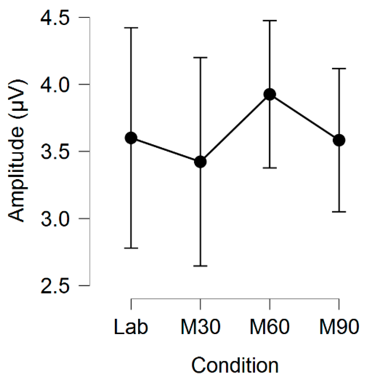
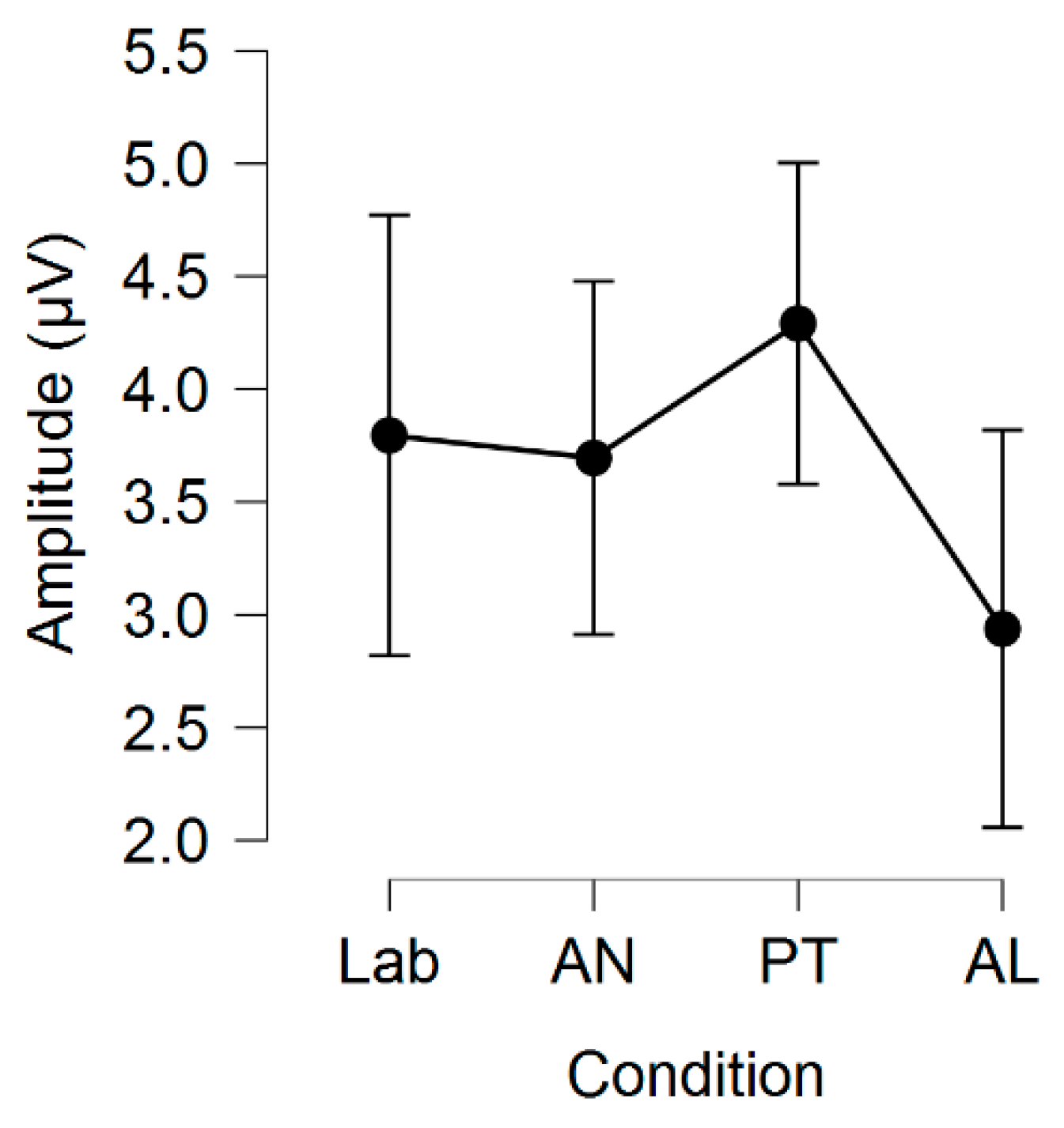
Table 1. The dependent variable amplitude was highest for
PT (4.29), followed by
M60 (3.93),
LC session 2 (3.80),
AN (3.70),
LC session 1 (3.60),
M90 (3.59),
M30 (3.43), and
AL (2.94), as portrayed in
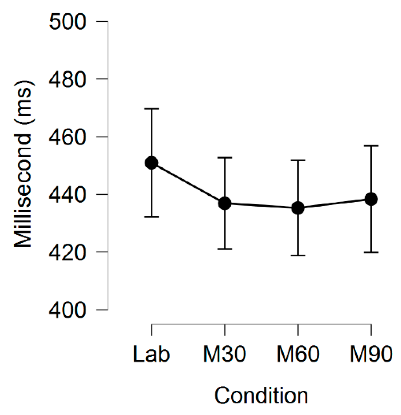
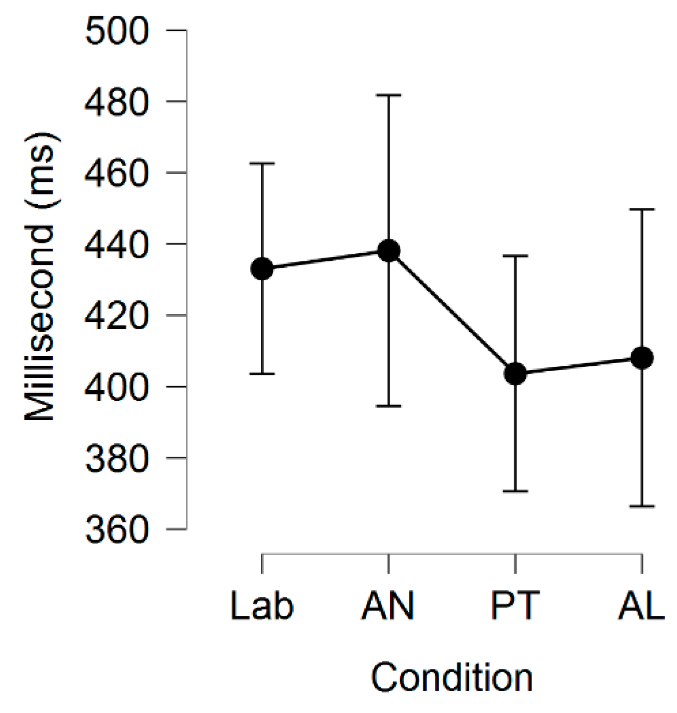
Table 11, while the latency was shortest for
PT, followed by
AL,
LC session 1,
LC session 2, M60,
M30,
M90, and
AN, as depicted in
Table 12. The user preference questionnaire (a) showed overwhelmingly that subjects preferred the
LC condition, as originally expected, followed by
M90,
M60,
AN,
M30,
AL, and
PT, and questionnaire (b) showed that subjects preferred
LC again, followed by
AN,
M90,
M60,
PT and
AL equally, and lastly
M30, as portrayed in
Table 13.
In this paper, we pursued the development of a hierarchical taxonomy aimed at categorizing distractions in the P300b domain, as depicted in
Figure 1. Explicitly, we examined the effect that the aforementioned independent variables, categorized under auditory distractions, have on the dependent variables. In the future, we plan to introduce additional types of distractions which are commonly found in a real-world environment and include them within the different categories of our taxonomy.


