Information Spread across Social Network Services with Non-Responsiveness of Individual Users

Abstract

This paper investigates the dynamics of information spread across social network services (SNSs) such as Twitter using the susceptible-infected-recovered (SIR) model. In the analysis, the non-responsiveness of individual users is taken into account; a user probabilistically spreads the received information, where not spreading (not responding) is equivalent to that the received information is not noticed. In most practical applications, an exact analytic solution is not available for the SIR model, so previous studies have largely been based on the assumption that the probability of an SNS user having the target information is independent of whether or not its neighbors have that information. In contrast, we propose a different approach based on a “strong correlation assumption”, in which the probability of an SNS user having the target information is strongly correlated with whether its neighboring users have that information. To account for the non-responsiveness of individual users, we also propose the “representative-response-based analysis”, in which some information spreading patterns are first obtained assuming representative response patterns of each user and then the results are averaged. Through simulation experiments, we show that the combination of this strong correlation assumption and the representative-response-based analysis makes it possible to analyze the spread of information with far greater accuracy than the traditional approach.

1. Introduction

When a major event occurs, a large number of original tweets and copies of these tweets commonly called “retweets” are posted on Twitter. Most tweets posted when a major event occurs are known to be retweets [1], and a large number of retweets are linked to a small number of original tweets describing the event. Posting retweets on a viral tweet getting many (thousands or more) retweets is very bursty: A large number of retweets are posted to the viral tweet in a short period of time. Such bursty spread of information, often referred to as information cascade, is found not only on Twitter but also on other social network services (SNSs). Understanding the information spread on Twitter through retweets is the first step toward understanding the more complex phenomena of information spread on SNSs.

In this paper, we investigate the spread of a piece of the target information, corresponding to an original (and viral) tweet on Twitter, using the susceptible-infected-recovered (SIR) model [2,3] with a given network topology representing the connections between SNS users. The SIR model is a mathematical epidemiological model originally designed for describing the spread of infectious diseases, but which can also be used to model the spread of information [3]. The simplicity of the SIR model makes it possible to analyze the spread of the target information by exactly taking into account the network topology. However, with the exception of very small networks, performing an exact analysis is impossible with the SIR model [3]. Therefore, in most existing studies on the spread of an epidemic disease [4,5,6,7,8], the probability that a given person is infected is assumed to be independent of whether its neighboring persons are infected. The assumption of the independence between neighbors is not appropriate for investigating the information spread on SNSs because SNS users are likely to form clusters [9] and whether or not each user knows the target information is strongly related to whether other members within the cluster know.

We previously proposed an approach not assuming independence between neighbors, in which the probability of a user knowing the target information is strongly correlated with whether its neighbors have that same information [10], which we call the “strong correlated assumption (SCA)”. In that work, we assumed that all users that received the target information broadcast it to their neighbors. In real situations, SNS users do not always respond to the information sent from their neighbors. Twitter users receive many tweets and retweets every day and these tweets/retweets are frequently overlooked (not noticed). This non-responsiveness of individual users should be considered in the model. Note that the original SIR model takes into account the non-responsiveness of individuals because a susceptible individual does not always become infected when interacting with an infected individual. In previous studies on epidemic spreading based on the SIR model, the response of each individual is first averaged and represented as a parameter often called the rate of infection, and then the spread of the epidemic is analyzed by solving differential equations with a given rate of infection.

Expanding the idea in our previous paper [10], we use the SIR model to analyze how the target information spreads in the presence of the non-responsiveness of individual users. In this paper, we investigate whether the SCA is still effective when accounting for the non-responsiveness of individual users. In addition to this, we investigate whether the conventional analysis, which solves differential equations with a given response rate (the rate of infection), is appropriate for taking into account the non-responsiveness of individual users. Accordingly, we propose an alternative approach called the “representative-response-based analysis”, where some information spreading patterns are first obtained assuming representative response patterns of each user and then the results are averaged, and we compare the representative-response-based analysis with the conventional analysis in terms of the accuracy of reproducing the simulation results. Note that this paper is an extended version of our recent conference paper [11].

The remainder of this paper is organized as follows. Section 2 briefly describes previous work on the SIR model and its application to the analysis of information spread on SNSs. Section 3 provides a mathematical model that explains the information spread on SNSs and proposes an analytical method based on the SCA and a new treatment of the responses of individual users. Section 4 outlines the results of simulations which show the superiority of the proposed analytical method over existing methods and Section 5 concludes the paper.

2. Previous Work

In the Susceptible-Infected-Susceptible (SIS) model, a person that is susceptible to contagion (S) can become infected (I) when exposed to an adjacent infected person. Infected persons may subsequently recover, but later become susceptible to reinfection. This state transition repeats until the whole network reaches a homogeneous stationary state. In the SIR model, persons are initially susceptible (S) to a contagion, and then may become infected (I) when exposed. However, the infected persons subsequently recover (R) and become resistant to the contagion. A large number of studies have been conducted on the spread of epidemic disease using the SIS or SIR model [3]. Among those, Anderson et al. [12] studied infectious diseases using both the SIS and SIR models based on mean-field approximation without explicitly considering network structures, while Pastor-Satorras et al. [13] and Boguna et al. [14] studied SIS and/or SIR models using node degree information, that is, the distribution of the number of neighboring persons. Based on this work, numerous studies have been conducted on SIS and SIR models in which network structures are directly considered via adjacency matrices [5,6,7,15,16].

Recently, several studies have been conducted on the spread of information over SNSs using the SIS and/or SIR models [17,18,19,20,21]. For example, Leskovec et al. [17] studied information spread through a social network over the Internet by examining the propagation patterns between blog posts using an information propagation model based on the SIS model. Cha et al. [18] investigated information cascades in Flickr, in which it often takes a long time for photo bookmarks to spread: an initial phase of exponential growth in the number of fans is followed by a phase of linear growth over several years. They showed that this phenomenon can be explained by the SEIR model, which has one additional state called exposed (denoted E), between the S and I states. In the exposed state, a user is more likely to access the photos in Flickr than in the susceptible state. Okada et al. [19] studied a topic propagation model based on the macroscopic SIS model which does not explicitly consider network structure, while Bauckhage et al. [20] investigated the change in people’s attention to viral videos from the point of view of mathematical epidemiology using the SIR model. Cheng et al. [21] performed an analysis of information cascades on Facebook over long time scales (almost one year) and showed that many such cascades recur, exhibiting multiple bursts of popularity, with periods of quiescence in between. They also showed that these phenomena could be explained by a revised SIR model in which resistant persons have a reduced risk of reinfection.

Retweet, which is the broadcasting of a received tweet to all followers, is the simplest way of spreading information, and the phenomenon observed on Twitter is the superposition of retweets on each original tweet. In this sense, understanding the broadcasting-based information spread is the first step toward understanding Twitter’s more complex phenomena. However, the broadcasting-based information spread has not been addressed in the previous studies on the information spread through social networks. Thus, in this paper, we focus on the broadcasting-based information spread using the SIR model explicitly considering the network topology. Explicitly considering the network topology in the analysis allows us to quantitatively discuss the phenomena on Twitter. Note that most of previous studies on the information spread using the SIS and/or SIR models take the macroscopic approach; they do not explicitly consider the network topology.

3. Information Spread on a Directed Network

3.1. Model Description

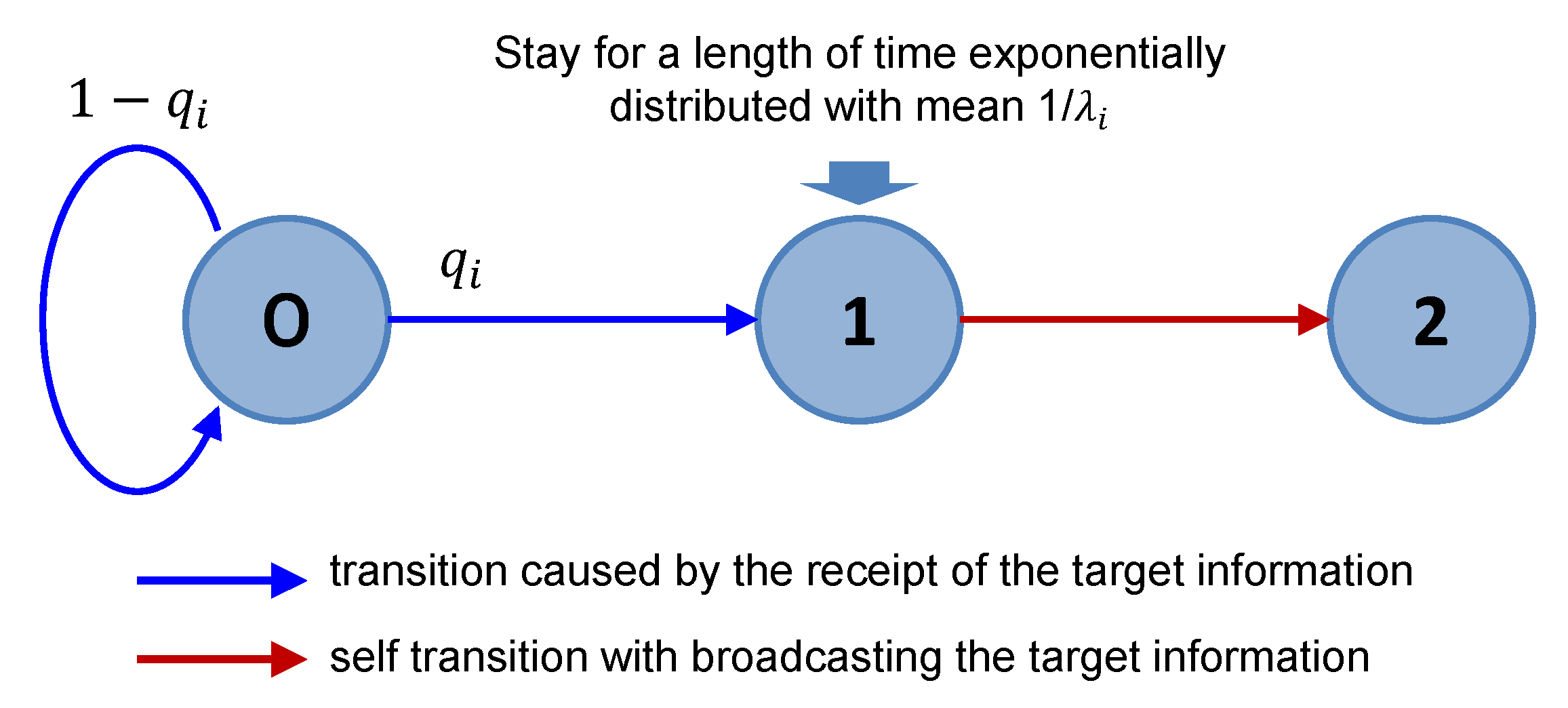
In this subsection, we consider the phenomenon in which a piece of information (such as an original tweet) spreads from an information holder on a directed network with N nodes where each such node is referred to as an agent; here, an agent corresponds to a user of an SNS who sends or receives the target information on the Internet. Each agent can be in one of the following three states, which are similar to the SIR model states:

State 0: 

Target information has not yet been received, or the information has been sent from neighbors but overlooked.

State 1: 

Target information has been received and will be spread in the subsequent time steps.

State 2: 

Target information has been received and spread.

At time 0, all agents except for the initial information holders are in state 0 and the initial information holders broadcast the target information for all their adjacent agents at time 0. If agent i receives the target information when it is in state 0, agent i ($i\in \mathcal{N}\stackrel{\mathrm{def}}{=}\{1,\dots ,N\}$) changes from state 0 to 1 with probability $q_i$. In what follows, $q_i$ is referred to as the response probability. Note that a transition from state 0 to 1 corresponds to the situation where agent i notices the target information and decides to spread it in the subsequent time. If agent i changes state from 0 to 1, it stays in state 1 for a set period of time. The length of time in which agent i stays in state 1 follows an exponential distribution with rate parameter $1/{\lambda }_i$. After staying in state 1 for this set period, agent i then broadcasts the target information to all adjacent agents, transitions from state 1 to state 2, and remains in that state without rebroadcasting the information. Note that, in this model, in reproducing information by retweeting on Twitter, the information is assumed to be spread by broadcasting (from one to many). The state transition diagram is given as Figure 1.

Although the above model is quite simple, it has the potential to explain real-world information spread on Twitter through retweets. Here, an example is presented to verify this claim. When Naomi Osaka, a tennis player with dual US and Japanese nationality, won the US Open in September 2018, a number of tweets were issued to mark her victory. Among those, a tweet issued by Shinzo Abe, Japanese Prime Minister, obtained over 20,000 retweets. The blue line in Figure 2 shows the actual number of retweets per 10-minute interval, while the red line shows what was predicted in this respect by the model. We assumed that ${\lambda }_i=\lambda$ and $q_i=q$ for all $i\in \mathcal{N}$, and $\lambda$ and q were time dependent. The time dependencies of $\lambda$ and q are depicted in Figure 3; these were manually determined so that the actual data (red line) roughly matches the simulation results (blue line). The simulation was conducted in a directional graph with 81,306 nodes and 1,786,149 links. The graph was constructed based on Twitter follower-followee data available in [22]. The figure shows that the results of the model (blue line) accord well with the real data (red line). The time dependence of parameters $\lambda$ and q is not explicitly considered in the analysis of this paper; rather, this example simply shows the potential applicability of the model to real-world phenomena.

3.2. Analysis

Let $A={\{a_{ij}\}}_{i,j\in \mathcal{N}}$ denote an adjacency matrix where $a_{ij}=1$ if a directed link exists from agent i to agent j; otherwise, $a_{ij}=0$. We also let $y_{ij}$ denote a random variable which is equal to 1 if agent j changes its state from 0 to 1 when it receives the target information from agent i; otherwise, $y_{ij}=0$. We let $E[y_{ij}]=q_j$ for all $i\in \mathcal{N}$, assuming that the probability that a user notices the received information (tweet) does not depend on the sender of the information. In what follows, $Y={\{y_{ij}\}}_{i,j\in \mathcal{N}}$ is referred to as the response matrix.

Hereinafter, we assume that the outcome of Y is known. That is, whether $y_{ij}=1$ or 0 is known for all $i,j\in \mathcal{N}$. This assumption is equivalent to cutting off the directed link from i to j if $y_{ij}=0$ and making the information spread on the resultant network without any users being non-responsive. This assumption is relaxed in Section 3.5.

The state of the network is expressed by $(Z_1(t),Z_2(t),\cdots ,Z_N(t))$, where $Z_i(t)$ denotes the state of agent i at time $t\ge 0$. The transition of $(Z_1(t),Z_2(t),\cdots ,Z_N(t))$ is governed by a continuous-time Markov chain. We define

$$X_i^{(k)}(t)=\left\{\begin{array}{cc}1,\hfill & Z_i(t)=k\hfill \\ 0.\hfill & \mathrm{otherwise}\hfill \end{array}\right.$$

With this definition, the probability that agent i is in state k at time t, $p_i^{(k)}(t)$, is given by

$$p_i^{(k)}(t)=E[X_i^{(k)}(t)].$$

Agent i changes its state from 0 to 1 only when it is in state 0 and (at least) one adjacent agent is in state 1. Agent i changes its state from 1 to 2 at a constant rate ${\lambda }_i$, but only when it is in state 1. This observation yields

$$\frac{d{p}_i^{(1)}(t)}{dt}=-{\lambda }_i{p}_i^{(1)}(t)+\sum _j{a}_{ji}{y}_{ji}{\lambda }_{j}E[X_j^{(1)}(t)X_i^{(0)}(t)],$$

(1)

$$\frac{d{p}_i^{(2)}(t)}{dt}={\lambda }_i{p}_i^{(1)}(t).$$

(2)

We define

$$\begin{array}{c}\hfill X_i(t)\stackrel{\mathrm{def}}{=}{X}_i^{(1)}(t)+X_i^{(2)}(t),p_i(t)\stackrel{\mathrm{def}}{=}E[X_i(t)].\end{array}$$

Note that $p_i(t)$ is the probability that agent i is in state 1 or 2 at time t; that is, agent i notices the target information sent from one of adjacent agents at time t. For later use, we prove the following identity.

Lemma 1.

$$a_{ji}{y}_{ji}{X}_j^{(2)}(t)X_i^{(0)}(t)=0.$$

(3)

Proof. 

Since (3) holds if $a_{ji}{y}_{ji}=0$ or $X_j^{(2)}(t)=0$, it is sufficient to prove (3) when $a_{ij}{y}_{ij}=1$ and $X_j^{(2)}(t)=1$. If $X_j^{(2)}(t)=1$, agent j has already sent the target information to all neighbor agents by time t and if $a_{ji}{y}_{ji}=1$, node i notices the target information, which is sent from node j. Thus, node i should be in state 1 or 2 at time t, that is, $X_i^{(0)}(t)=0$, which completes the proof. □

Summing (1) and (2) yields

$$\begin{array}{cc}\frac{d{p}_i(t)}{dt}\hfill & =\sum _j{a}_{ji}{y}_{ji}{\lambda }_{j}E[X_j^{(1)}(t)X_i^{(0)}(t)]\hfill \\ \hfill & =\sum _j{a}_{ji}{y}_{ji}{\lambda }_{j}E[(X_j^{(1)}(t)+X_j^{(2)}(t))X_i^{(0)}(t)]\hfill \\ \hfill & =\sum _j{a}_{ji}{y}_{ji}{\lambda }_{j}E[(X_j^{(1)}(t)+X_j^{(2)}(t))(1-X_i^{(1)}-X_i^{(2)}(t))]\hfill \\ \hfill & =\sum _j{a}_{ji}{y}_{ji}{\lambda }_{j}E[X_j(t)(1-X_i(t))]\hfill \\ \hfill & =\sum _j{a}_{ji}{y}_{ji}{\lambda }_j(p_j(t)-E[X_j(t)X_i(t)]),\hfill \end{array}$$

(4)

where the second equality comes from Lemma 1 and the third equality comes from $X_i^{(0)}+X_i^{(1)}+X_i^{(2)}=1$.

Remark 1.

In the original SIR model, the spread of infection from an infected agent to its adjacent agents occurs independently at different times, which is different from the model described in this paper. Note that the information spread (spread of infection disease) is faster in the original SIR model than in the model considered in this paper. To see the difference, consider an agent (agent A) having two adjacent agents (agents B and C). Assume that agent A in state 1 at time t, and agents B and C are both in state 0 at time t. In the original SIR model, agent B receives the information at time $t+T_B$ and agent C receive the information at time $t+T_C$, where $T_B$ and $T_C$ are mutually independent and exponentially distributed random variables with mean $1/\lambda$. In the model considered in this paper, agents B and C simultaneously receive the information at time $t+T$, where T is an exponentially distributed random variable with mean $1/\lambda$. Since $min\{T_B,T_C\}$ is stochastically smaller than T, the information transfer in the original SIR model stochastically occurs faster than in the considered model.

3.3. Strong Correlation Assumption

Here, the exact value of $p_i(t)$ cannot be obtained by solving (4) because the $E[X_i(t)X_j(t)]$ term is not known. However, the upper and lower bounds of $p_i(t)$ can be obtained using the following lemma.

Lemma 2.

If $X_i(t)$ and $X_j(t)$ are non-negatively correlated, that is, they satisfy $\mathrm{Cov}[X_i(t),X_j(t)]\ge 0$, then

$$p_i(t)p_j(t)\le E[X_i(t)X_j(t)]\le min\{p_i(t),p_j(t)\}.$$

Proof. 

From the fact that $X_i(t)$ and $X_j(t)$ are non-negatively correlated, it follows that

$$\begin{array}{cc}\hfill \mathrm{Cov}\left[X_i(t),X_j(t)\right]& =E\left[X_i(t)X_j(t)\right]-E\left[X_i(t)\right]E\left[X_j(t)\right]\ge 0,\hfill \end{array}$$

which means that $p_i(t)p_j(t)\le E[X_i(t)X_j(t)]$. It is also seen that

$$\begin{array}{cc}E\left[X_i(t)X_j(t)\right]\hfill & =P\left(\{X_i(t)=1\}\cap \{X_j(t)=1\}\right)\hfill \\ \hfill & \le P\left(\{X_i(t)=1\}\right)=p_i(t),\hfill \end{array}$$

(5)

and

$$\begin{array}{cc}E[X_i(t)X_j(t)]\hfill & =P\left(\{X_i(t)=1\}\cap \{X_j(t)=1\}\right)\hfill \\ \hfill & \le P\left(\{X_j(t)=1\}\right)=p_j(t).\hfill \end{array}$$

(6)

(5) and (6) yield

$$E[X_i(t)X_j(t)]\le min\{p_i(t),p_j(t)\},$$

which completes the proof. □

Most recent related studies have solved (4) by assuming $p_i(t)p_j(t)=E[X_i(t)X_j(t)]$ (or by using assumptions similar to this) [15,16,23,24,25], which is called the independence assumption (IA) in this paper. In contrast, here we assume $E[X_i(t)X_j(t)]=min\{p_i(t),p_j(t)\}$, which we refer to as the strong correlation assumption (SCA). To the best of the authors’ knowledge, no previous studies have considered this assumption. Under this assumption, (4) is expressed as

$$\begin{array}{cc}\frac{d{p}_i(t)}{dt}\hfill & =\sum _j{a}_{ji}{y}_{ji}{\lambda }_j(p_j(t)-min\{p_i(t),p_j(t)\})\hfill \\ \hfill & =\sum _{j;p_j(t)>p_i(t)}{a}_{ji}{y}_{ji}{\lambda }_j(p_j(t)-p_i(t)).\hfill \end{array}$$

(7)

The second line of the above equation means that the target information from agent i is received and noticed by agent j when $p_j(t)>p_i(t)$. In other words, the SCA describes the target information spread from the agents that are most likely to have the target information to agents that are most unlikely to have the target information. It also gives the lower bound for the probability that an agent has the target information, while the IA provides the upper bound of the probability.

3.4. Upstream and Downstream Relationship

Here, we introduce the following order relationship between agents, which is referred to as the upstream and downstream relationship in this paper.

Definition 1.

(upstream and downstream relationship). If $X_j(t)\ge X_i(t)$ for all t, we say that agent i is downstream of agent j (agent j is upstream of agent i) and denote this by $j\to i$.

If the upstream and downstream relationship exists for each pair of adjacent agents, the SCA gives the exact result. To show this, without loss of generality, we assume that agent j is upstream of agent i ($j\to i$). Note that $p_j(t)\ge p_i(t)$ if $j\to i$ because $\{X_j(t)=1\}\supset \{X_i(t)=1\}$. We also see that

$$\begin{array}{cc}\hfill E[X_i(t)X_j(t)]& =P\left(\{X_i(t)=1\}\cap \{X_j(t)=1\}\right)\hfill \\ \hfill & =P\left(\{X_i(t)=1\}\right)=p_i(t)=min\{p_i(t),p_j(t)\},\hfill \end{array}$$

which means that the SCA exactly holds. In addition to this, if the upstream and downstream relationship exists for all pairs of adjacent agents, (7) holds for all t and thus we have

$$\begin{array}{cc}\hfill {\int }_0^{\infty }\frac{d{p}_i(t)}{dt}{e}^{-st}dt& =\sum _{j;j\to i}{\int }_0^{\infty }{a}_{ji}{y}_{ji}{\lambda }_j(p_j(t)-p_i(t))e^{-st}dt.\hfill \end{array}$$

If i is not the initial information holder (that is, $p_i(0)=0$), we obtain

$$s{p}_i^{*}(s)=\sum _{j;j\to i}{a}_{ji}{y}_{ji}{\lambda }_j(p_j^{*}(s)-p_i^{*}(s)),$$

(8)

where $p_i^{*}(s)$ is the Laplace-Stieltjes transform of $p_i(t)$ defined as follows:

$$p_i^{*}(s)\stackrel{\mathrm{def}}{=}{\int }_0^{\infty }\frac{d{p}_n(t)}{dt}{e}^{-st}dt={\int }_0^{\infty }{e}^{-st}d{p}_n(t).$$

Note that $p_i(s)=1$ if i is the initial information holder because $p_i(t)=1$ for $t\ge 0$ and $p_i(t)=0$ for $t<0$.

The upstream and downstream relationship exists for all pairs of adjacent agents when the target information is spread over a tree-topology network from its root (Figure 4). Assume that agent i is located n hops downstream from the root, and the path from the root to agent i is given by

$$i_0\to i_1\to ,\dots ,\to i_n,$$

where $i_0$ is the root and $i_n=i$. It follows from (8) that

$$p_{i_k}^{*}(s)=\frac{y_{i_{k-1}{i}_k}{\lambda }_{i_{k-1}}}{s+y_{i_{k-1}{i}_k}{\lambda }_{i_{k-1}}}{p}_{i_{k-1}}^{*}(s),k=1,\cdots ,n$$

and thus we obtain

$$p_i^{*}(s)=\prod _{k=1}^n\frac{y_{i_{k-1}{i}_k}{\lambda }_{i_{k-1}}}{s+y_{i_{k-1}{i}_k}{\lambda }_{i_{k-1}}}=\left\{\begin{array}{cc}\prod _{k=1}^n\frac{{\lambda }_{i_{k-1}}}{s+{\lambda }_{i_{k-1}}},\hfill & \prod _{k=1}^n{y}_{i_{k-1}{i}_k}=1\hfill \\ 0.\hfill & \mathrm{otherwise}\hfill \end{array}\right.$$

In particular, if ${\lambda }_{i_k}=\lambda$ for all $k=1,\cdots ,n$, it is possible to analytically retransform $p_i^{*}(s)$ to $p_i(t)$, and the closed-form representation of $p_i(t)$ is obtained as follows:

$$p_i(t)=\left\{\begin{array}{cc}\sum _{k=0}^{n-1}\frac{{(\lambda t)}^k}{k!}{e}^{-\lambda t},\hfill & \prod _{k=1}^n{y}_{i_{k-1}{i}_k}=1\hfill \\ 0.\hfill & \mathrm{otherwise}\hfill \end{array}\right.$$

3.5. Taking the Average on the Response Matrix

Let $L(t)$ be the number of agents that have spread the target information by time t, which corresponds to the number of retweets posted by time t after the original tweet was posted at time 0. The information cascade can be described by $L(t)$. Since $L(t)={\sum }_i{X}_i^{(2)}(t)$, the conditional expectation of $L(t)$ on the response matrix Y, $E[L(t)|Y]$, is calculated as

$$E[L(t)|Y]=\sum _{i}E[X_i^{(2)}(t)|Y]=\sum _i{p}_i^{(2)}(t|Y),$$

where $p_i^{(2)}(t|Y)$ is the conditional probability that agent i is in state 2 given the outcome of Y. Note that the results in the previous subsections also have dependence on the outcome of Y and thus, for example, $p_i(t)$ in (4) should be written as $p_i(t|Y)$ in a rigorous sense. We did not, however, use this rigorous notation in the previous subsections for simplicity of expression. Let $T_i$ be the time at which agent i received the target information and let ${\tau }_i$ be the period between the time when agent i receives and spreads the target information. We have

$$\begin{array}{cc}\hfill p_i^{(2)}(t|Y)& =P(T_i+{\tau }_i\le t|Y)\hfill \\ \hfill & ={\int }_0^{t}P(T_i\le t-u|Y)P(s\le {\tau }_i<u+du|Y)\hfill \\ \hfill & ={\int }_0^t{\lambda }_{i}P(T_i\le t-u|Y)e^{-{\lambda }_{i}u}du\hfill \\ \hfill & ={\int }_0^t{\lambda }_i{p}_i(t-u|Y)e^{-{\lambda }_{i}u}du={\int }_0^t{\lambda }_i{p}_i(u|Y)e^{-{\lambda }_i(t-u)}du.\hfill \end{array}$$

Thus,

$$E[L(t)|Y]=\sum _i{\int }_0^t{\lambda }_i{p}_i(u|Y)e^{-{\lambda }_i(t-u)}du,$$

(9)

where, as previously noted, $p_i(t|Y)$ is the same as $p_i(t)$ in the previous sections because the outcome of Y is assumed to be given in the previous sections. Note that $p_i(t|Y)$ can be obtained by numerically solving (7) if Y is given.

To obtain $E[L(t)]$, we need to calculate $E[L(t)|Y]$ for all possible outcomes of Y and sum the results using weights which equal the probability of the outcome. Calculating $E[L(t)|Y]$ for all possible outcomes of Y is, however, impossible because the number of possible outcomes of Y increases exponentially with the number of agents in the network. One possible approach for approximately calculating $E[L(t)]$ is to obtain ${\{p_i(u)\}}_{i=1}^N={\{E[p_i(u|Y)]\}}_{i=1}^N$ through (4) by assuming that $y_{ji}$ is equal to the response probability, that is, $y_{ij}=q_i(=E[y_{ji}])$. Under this assumption, ${\{p_i(t)\}}_{i=1}^N$ is approximately given as the solutions to the following differential equations:

$$\begin{array}{cc}\hfill \frac{d{p}_i(t)}{dt}& =\sum _j{a}_{ji}{q}_i{\lambda }_j(p_j(t)-E[X_j(t)X_i(t)]),i\in \mathcal{N}.\hfill \end{array}$$

(10)

By applying the SCA (or IA) to the above, we can numerically obtain ${\{p_i(t)\}}_{i=1}^N$. Once ${\{p_i(u)\}}_{i=1}^N$ is obtained, we can calculate $E[L(t)]$ by using the following relationship:

$$E[L(t)]=\sum _i{\int }_0^t{\lambda }_i{p}_i(u)e^{-{\lambda }_i(t-u)}du.$$

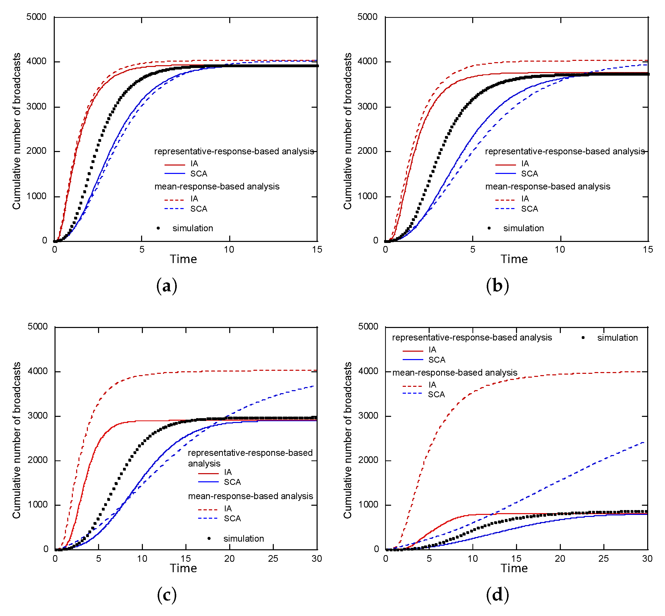
Most previous studies on epidemic spreading using the SIS model or SIR model [4,5,6,7,8] adopted the assumption $y_{ij}=q_i(=E[y_{ji}])$. The response of each individual is first averaged and represented as a parameter $q_i$, which is often called the rate of infection, and then the spread of the epidemic is analyzed by solving differential equations similar to (10). We call this approach the “mean-response-based analysis”. Unfortunately, as shown in the next section, this analytical approach greatly overestimates $E[L(t)]$ especially when $q_i$ is equal to or less than 0.1. The mean-response-based analysis implicitly assumes that $y_{ij}$ and $E[X_j(t)X_i(t)|Y]$ are statistically independent, but this assumption does not hold, resulting in a discrepancy between the simulation results and the mean response-based analysis.

Another possible approach is to calculate $E[L(t)|Y]$ for some (randomly selected) outcomes of Y and take their average. This approach, called the “representative-response-based analysis” in this paper, corresponds to the notion that some information spreading patterns are first obtained assuming representative response patterns of each user and then the results are averaged. Surprisingly, as shown in the next section, the dependence of $E[L(t)]$ on the outcome of Y is very small for large networks and the representative-response-based analysis yields a much better estimate of $E[L(t)]$ than the mean-response-based analysis.

Note that the exact result is available when the target information is spread over a tree-topology network from its root (Figure 4). For example, if the path from the root to agent i is $i_0\to i_1\to ,\dots ,\to i_n=i$, and ${\lambda }_{i_k}=\lambda$ for all $k=1,\cdots ,n$, then

$$p_i(t)=\left(\prod _{k=1}^n{q}_{i_k}\right)\sum _{k=0}^{n-1}\frac{{(\lambda t)}^k}{k!}{e}^{-\lambda t}.$$

3.6. Mean-Field Approximation

Under the IA $E[X_i(t)X_j(t)]=p_i(t)p_j(t)$ and SCA $E[X_i(t)X_j(t)]=min\{p_i(t),p_j(t)\}$, interpolating both approximations with linear equations using the parameter $\alpha$ yields

$$E[X_i(t)X_j(t)]=(1-\alpha )p_i(t)p_j(t)+\alpha min\{p_i(t),p_j(t)\}.$$

(11)

Setting $\alpha =0$ in the above equation gives the IA, while setting $\alpha =1$ gives the SCA. Among the two approximations mentioned in Section 3.5, we use the first one and apply (11) to get

$$\begin{array}{cc}\hfill \frac{d{p}_i(t)}{dt}& =\sum _j{a}_{ji}{q}_i{\lambda }_j(p_j(t)-(1-\alpha )p_i(t)p_j(t)+\alpha min\{p_i(t),p_j(t)\}).\hfill \end{array}$$

(12)

Applying the mean-field approximation, where $p_i(t)=p(t)$, ${\lambda }_i=\lambda$, and $q_i=q$ for all $i\in \mathcal{N}$, to (12), yields

$$\begin{array}{cc}\hfill \frac{dp(t)}{dt}& =dq\lambda (p(t)-(1-\alpha )p{(t)}^2-\alpha p(t))\hfill \\ \hfill & =dq\lambda (1-\alpha )p(t)(1-p(t)),\hfill \end{array}$$

in which d is the mean degree of the agent. The above differential equation has the following solution:

$$p(t)=\frac{p(0)}{p(0)+(1-p(0))e^{-dq\lambda (1-\alpha )t}}.$$

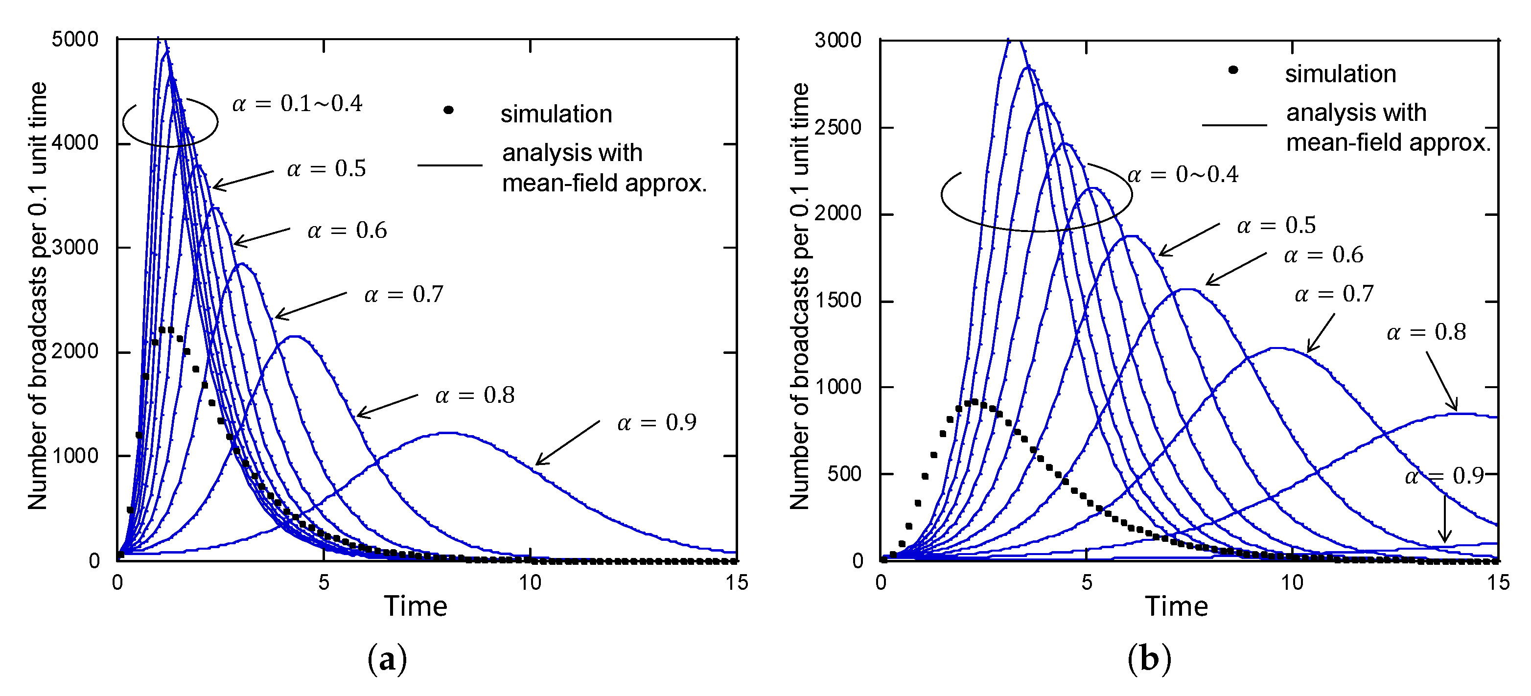
This result shows that the probability that an agent will have received the target information by time t follows a logistic curve as per what appears in population growth models. In addition to this, $\alpha$ acts as a scale parameter of time t, and larger $\alpha$ (which means the approximation is closer to the SCA has the effect of advancing the time more slowly. The expectation for the total number of agents that have spread the target information up to time t can then be calculated by the following equation:

$$E[L(t)]={\int }_0^t\frac{N\lambda p(0)e^{-\lambda (t-s)}}{p(0)+(1-p(0))e^{-dq\lambda (1-\alpha )s}}ds.$$

(13)

4. Simulation and Discussion

4.1. Outline of the Simulation

To evaluate the accuracy of the analytical methods explained in Section 3, we conducted simulation experiments for the target information spread based on the model described in Section 3.1. We configured two different graphs based on the data available in [22]. The first graph (called the Facebook network) represents a social network (friendship relations) on Facebook and the other (called the Twitter network) represents a followee-follower network on Twitter. The Facebook network has 4039 nodes and 88,234 links, and the Twitter network has 81,306 nodes and 1,768,149 links. The target information spread started from broadcasting by a single information source (node). The outdegree of the information source was 30 for the Facebook network, and 1111 for the Twitter network. We chose these two networks because Facebook and Twitter are representative SNSs. Also, because the Facebook network is smaller than the Twitter network, the network size dependence of the accuracy of the proposed analysis can be seen from the results of these two networks.

The pseudo code of the simulation is shown as Algorithm 1, where $S_0$, $S_1$, and $S_2$ respectively denote the sets of agents in states 0, 1, and 2, and $t_i$ denotes the time at which agent i broadcasts the target information. $RAND(0,1)$ is one random number extracted from a uniform distribution on $[0,1]$, and $EXP(x)$ is one random number extracted from the exponential distribution with mean x. In Algorithm 1, we assume that agent 1, the information source, is in state 1 and all agents except agent 1 are in state 0 at time 0. As shown in Algorithm 1, the procedure of the simulation is very simple. When an agent receives the target information while in state 0, the agent changes from state 0 to state 1 with probability $q_i$. After changing state from 0 to 1, the agent stays in state 1 for some period of time and then broadcasts the target information to all adjacent agents. After broadcasting, the agent changes from state 1 to state 2 and stays in that state, never broadcasting the information again. The simulation stops when no agent is in state 1, that is, when no other agents will broadcast the target information. The pseudo code has two sets of parameters, ${\{{\lambda }_i\}}_{i\in \mathcal{N}}$ and ${\{q_i\}}_{i\in \mathcal{N}}$, where ${\lambda }_i$ is the mean length of the period that agent i stays in state 1 and $q_i$ is the response probability. In the simulations, we set ${\lambda }_i=1$ for all $i\in \mathcal{N}$. Settings of ${\{q_i\}}_{i\in \mathcal{N}}$ will be considered in the subsequent subsections.

We conducted the simulations using an event-driven simulator written in C on a machine running an Intel Xeon E5-1650 processor (3.5 GHz). The results obtained in the simulation, namely the number of broadcasts per 0.1 time units and the cumulative number of broadcasts, were compared with the results obtained by the proposed analysis.

Algorithm 1 Pseudo Code of Simulation for Information Spread

Initialization:$S_0=\mathcal{N}\backslash \{1\},S_1=\{1\},S_2=\varnothing ,t_1=0$   1: while$S_1\ne \varnothing$do   2:  Select $i\in S_1$ such that $\forall j\in S_1,t_i\le t_j$   3:  for all $j\in S_0$ do   4:   $r_j=RAND(0,1)$   5:   if $a_{ij}=1$ and $r_j\le q_j$ then   6:    $S_1=S_1\cup \{j\},S_0=S_0\backslash \{j\},t_j=t_i+EXP(1/{\lambda }_j)$   7:   end if   8:  end for   9:  $S_1=S_1\backslash \{i\},S_2=S_2\cup \{i\}$   10: end while

4.2. Result: Response Probability ($q=1$)

We first conducted simulation experiments for the case where the response probability of each agent is equal to one; that is, all agents in state 0 transit to state 1 when they receive the target information from their neighbors. Figure 5a shows the temporal evolution of the number of agents spreading the target information, $E[L(t)]$, for the Facebook network. Note that the vertical axis shows not $E[L(t)]$, but the net increase of $E[L(t)]$ during a period of 0.1 time units (that is, $E[L(t+0.1)-L(t)]$). Each filled circle shows the average of the results of 1000 simulations, each of which was conducted with a different seed in the random number generator algorithm. The red and blue solid curves show the analytical results under the SCA and the IA, respectively. Note that we do not need to take the average for the response matrix, Y, for the case where the response probability is equal to one. Figure 5a shows a typical information cascade in which the number of agents that spread the target information increases rapidly, reaches a peak, and then gradually decreases. It also shows that an analysis based on the SCA reproduces the simulation results much more accurately than an analysis based on the IA.

Figure 5b shows the results for the Twitter network. The SCA-based and IA-based analyses both accurately reproduce simulation results, although the former is somewhat better than the latter.

4.3. Results: Response Probability ($q<1$)

We next conducted simulations for the case where the response probability was less than 1, that is, all agents in state 0 probabilistically transit to state 1 when they receive the target information from their neighbors. For simplicity, we assumed that all agents had the same response probability, that is, $q_i=q$ for all $i\in \mathcal{N}$, and we conducted four sets of simulations by setting q at four different values: 0.5, 0.3, 0.1, and 0.05. The time change of the number of broadcasts per 0.1 time units and the cumulative number of broadcasts $E[L(t)]$ for the Facebook network are respectively shown in Figure 6 and Figure 7. The circles show the simulation results, while solid and dotted lines show the analytical results. Note that for the case where the response probability is less than 1, we need to use an approximation for the average of response matrix Y as explained in Section 3.5. The blue (SCA) and red (IA) solid curves show the results from the representative-response-based analysis, in which the $E[L(t)|Y]$ are obtained for ten different outcomes of Y and the results are averaged to yield the final result. We checked the randomness of the ten outcomes of Y by using the following index:

$$\begin{array}{c}Cov[Y^{(m)},Y^{(n)}]\stackrel{\mathrm{def}}{=}\frac{{\sum }_{i,j}{a}_{ij}(y_{ij}^{(m)}-\overline{Y^{(m)}})(y_{ij}^{(n)}-\overline{Y^{(n)}})}{\sqrt{Var[Y^{(m)}]}\sqrt{Var[Y^{(n)}]}}\hfill \\ \overline{Y^{(m)}}\stackrel{\mathrm{def}}{=}\frac{{\sum }_{i,j}{a}_{ij}{y}_{ij}^{(m)}}{{\sum }_{i,j}{a}_{ij}},Var[Y^{(m)}]\stackrel{\mathrm{def}}{=}\frac{{\sum }_{i,j}{a}_{ij}(y_{ij}^{(m)}-\overline{Y^{(m)}})(y_{ij}^{(m)}-\overline{Y^{(m)}})}{{\sum }_{i,j}{a}_{ij}}\hfill \end{array}$$

(14)

where $Y^{(m)}={\{y^{(m)}\}}_{i,j\in \mathcal{N}}$ is the mth outcome of the response matrix. Note that if $Y^{(m)}$ is identical with $Y^{(n)}$, then $Cov[Y^{(m)},Y^{(n)}]=1$. The index defined above was within $[-0.01,0.01]$ for all pairs of the ten outcomes of Y, meaning that the ten outcomes were statistically independent. The blue (SCA) and red (IA) dashed curves show the results from the mean-response-based analysis.

In the figures, we see that the dashed curves are not consistent with the simulation results compared with the solid curves. In particular, Figure 7 shows that the dashed curves overestimate the cumulative number of broadcasts more as q becomes smaller. Among the four curves, the red dashed curve (combination of the mean-response-based analysis and the IA) deviates the most by far from the simulation results, and the blue solid curve (combination of the representative-response-based analysis and the SCA) best agrees with the simulation results when $q=0.1$ and $q=0.05$.

The results for the Twitter network are shown in Figure 8 and Figure 9. As in the case of the Facebook network, the dashed curves are inconsistent with the simulation results compared with the solid curves when $q=0.1$ and $q=0.05$. In particular, as shown in Figure 9, the dashed curves significantly overestimate the cumulative number of broadcasts when $q=0.1$ and $q=0.05$. These results show that the mean-response-based analysis is not suitable especially when the response probability is around 0.1 or smaller. As we mentioned in Section 3.1, the number of retweets of the original tweet issued by Japanese Prime Minister Shinzo Abe celebrating Naomi Osaka’s victory at the US Open in September 2018 is well reproduced by the SIR model when the response probability is set at values from 0.05 to 0.1. In general, the response probabilities of Twitter users are small, being at most 0.1 [26].

Figure 8 and Figure 9 indicate that, for the Twitter network, the simulation results are midway between the red solid curve and blue solid curve. These two curves give good approximations of the simulation results regardless of the response probability setting.

4.4. Dependence on Response Matrix Outcome

As shown in Section 4.3, the representative-response-based analysis yields better results than the mean-response-based analysis. However, there is a concern regarding the former analysis that the information spread may vary greatly depending on the choice of the outcome of Y. To discern the dependence of information spread on the outcome of Y, in Figure 10 (Facebook) and Figure 11 (Twitter), we present five simulation results, which were separately obtained for five different outcomes of Y (five different sets of values of ${\{y_{ij}\}}_{i,j\in \mathcal{N}}$). Note that the five outcomes are chosen from the ten outcomes of Y which are used in the analysis in Section 4.3. As the figures indicate, for the Facebook network, the dependence on the outcome of Y is very small when $q=0.3$. In addition to this, the dependence of the information spread on the outcome of Y for the Twitter network is almost negligible. These results support the validity of the representative-response-based analysis especially when it is applied to large-size networks such as that of Twitter. Furthermore, these results suggest that, in the representative-response-based analysis, it is not necessary to obtain results for multiple outcomes of Y and then take their average; it is sufficient to take the result for one (randomly selected) outcome of Y.

Note that the outgoing degree of the information source in the Facebook network is 30. This causes the large dependence of the information spread on the outcome of the response matrix when $q\le 0.1$ for the Facebook network. The number of the first recipients is equal to the outgoing degree of the information source. The probability that all of the first recipients do not respond to the target information is equal to ${(1-q)}^n$, where n denotes the outgoing degree of the information source. This no-response probability is equal to 0.21 when $q=0.05$ and $n=30$. In fact, the number of broadcasts was equal to zero in the case of outcome $Y^{(3)}$ in Figure 10c, where none of the first recipients of the target information responded to the information. The degree of the information source in the Twitter network is 1111, so some of the first recipients should respond to the information even if q is less than 0.1. The representative-response-based analysis is thus applicable if the number of neighbor users (e.g., followers in Twitter) of the information source is several hundreds or larger even if the response probability is less than 0.1. When the representative-response-based analysis is applied to the case where the number of neighbor users of the information source is small, we should evaluate the information spread for various outcomes of the response matrix and take their average.

4.5. Mean-Field Approximation

Finally, we show the analytical results for the mean-field approximation (Equation (13)) in Figure 12 (Facebook) and Figure 13 (Twitter). Each figure shows ten different results with the mean-field approximation, which were obtained by varying the parameter $\alpha$ from 0 to 0.9 in increments of 0.1. These figures show that the simulation results are not consistent with the results of mean-field approximation for any value of $\alpha$. Especially when $q=0.1$, the results of mean-field approximation greatly overestimate the number of broadcasts. This is because the mean-field approximation uses the mean-response-based analysis. These numerical examples reveal that the mean-field approximation is not suitable for quantitatively estimating the information spread especially when the response probability is around 0.1 or smaller.

5. Conclusions

In this paper, we described a method of mathematically analyzing information propagation on an SNS based on the SIR model. In particular, we proposed an analysis method that can consider the existence of users who do not respond to the target information. Mathematically taking into account users who do not respond to the target information is not trivial. In fact, as shown in this paper, the conventional approach (mean-response-based analysis) produces large errors, especially when the response probability is small ($q\le 0.1$). The representative-response-based analysis, newly proposed in this paper, is especially useful for analyzing information spread in large-size networks because it includes much less error than the conventional approach. The representative response-based analysis relies on the fact that the number of broadcasts per unit of time does not depend on the details of the outcome of the reaction matrix, especially for large-size networks. We expect that there is a mathematical law such as the law of large numbers behind this fact, but finding this mathematical law is a future subject. We also found that the SCA [10] is still effective in the presence of non-responsive users. However, we also found that the information spread in the presence of non-responsive users is roughly midway between the SCA and the IA results. The development of a method to analyze the information spread with higher accuracy by combining the SCA and the IA is a future task. We also note that the proposed analysis is applicable to the case where the parameters, $\lambda$ and q, have time dependence, but whether the proposed analysis can reproduce simulation results when time dependence of the parameters exists is to be investigated as a future study. Further, it would be interesting to apply machine learning, including deep learning, to identify the parameters of the proposed model ($\{{\lambda }_i\}$ and $\{q_i\}$) from real-time data on tweets and retweets so as to predict how the number of tweets will increase in the future.