Improved Measures of Redundancy and Relevance for mRMR Feature Selection

Abstract

Many biological or medical data have numerous features. Feature selection is one of the data preprocessing steps that can remove the noise from data as well as save the computing time when the dataset has several hundred thousand or more features. Another goal of feature selection is improving the classification accuracy in machine learning tasks. Minimum Redundancy Maximum Relevance (mRMR) is a well-known feature selection algorithm that selects features by calculating redundancy between features and relevance between features and class vector. mRMR adopts mutual information theory to measure redundancy and relevance. In this research, we propose a method to improve the performance of mRMR feature selection. We apply Pearson’s correlation coefficient as a measure of redundancy and R-value as a measure of relevance. To compare original mRMR and the proposed method, features were selected using both of two methods from various datasets, and then we performed a classification test. The classification accuracy was used as a measure of performance comparison. In many cases, the proposed method showed higher accuracy than original mRMR.

1. Introduction

Recently, with the rapid development of machine learning and the increasing accumulation of data through the internet, various methods of analyzing data using past techniques have been difficult to apply to modern big data problems, and various data preprocessing techniques have been developed. Among them, feature selection is a process of selecting a set of features (variables, attributes) that meet the purpose of analysis for a high-dimensional dataset having thousands or tens of thousands of features. Analysts can benefit from a selection of features, including better performance of predictive models, and faster and more efficient data analysis. The advantages of feature selection are as follows:

(a)

reduces the dimension of the dataset and therefore reduces the cost of computing resources

(b)

improves classification model performance by reducing data noise

(c)

facilitates data visualization and understanding

The main purpose of the general feature selection is to determine a set of related features that is of interest regarding particular events or phenomena. This feature selection is usually divided into filtering methods and wrapper methods, depending on how the relevant features are searched [1,2,3,4]. Filter techniques assess the relevance of features by evaluating only the intrinsic properties of the data [1]. In most cases, relevance scores between each feature and class vector are calculated, and high-scored features are selected. Filter techniques are simple, fast, and easy to understand. However, they do not consider redundancy and interaction between features; they assume features are independent from each other. To capture the interactions between features, wrapper methods embed a classification model within the feature subset evaluation. However, as the space of feature subsets grows exponentially with the number of features, heuristic search methods such as forward search and backward elimination are used to guide the search toward an optimal subset [1]. Feature selection can be categorized into supervised, unsupervised, and semisupervised [5,6,7]. Supervised feature selection algorithms consider features’ relevance by evaluating their correlation with the class information whereas unsupervised feature selection algorithms may exploit data variance or data distribution in its evaluation of features’ relevance without labels. Semisupervised feature selection algorithms use a small amount of labeled data as additional information to improve unsupervised feature selection [5]. Minimum Redundancy Maximum Relevance (mRMR) and the proposed method belong to the supervised method.

Ding and Hanchuan [8,9] suggested the mRMR measure to reduce redundant features during the feature selection process. They tried to measure both redundancy among features and relevance between features and class vector for a given set of features. Their redundancy and relevance measures are based on mutual information as follows:

$$I\left(x,y\right)={\sum }_{i,j}log\frac{p\left(x_i,y_j\right)}{p\left(x_i\right)p\left(y_j\right)}$$

(1)

In the Equation (1), x and y are feature vector or class vector, and p() represents probability. Suppose S is a given set of features and h is a class variable. The redundancy of S is measured by Equation (2):

$$W_i=\frac{1}{{\left|S\right|}^2}{\sum }_{i,j\in S}I\left(i,j\right)$$

(2)

In Equation (2), |S| is the number of features in S. The relevance of S is measured by Equation (3):

$$V_I=\frac{1}{\left|S\right|}{\sum }_{i\in S}I\left(h,i\right)$$

(3)

There are two types of methods to evaluate S:

$$\mathrm{MID}:V_I-W_I$$

(4)

$$\mathrm{MIQ}:V_I/W_I$$

(5)

In many cases, MIQ (Mutual Information Quotient) shows better performance than MID (Mutual Information Difference). We cannot test all subsets of features S for a given dataset, so the mRMR algorithm adopts a forward search in its implementation. The procedure is described in Algorithm 1.

Algorithm 1: Forward search

/*

M: size of feature subset S that we want to get

S: set of selected features

F: whole set of features of target dataset

*/

S ← ∅

REPEAT UNTIL |S| < M

Find fi∈F that maximize MID/MIQ of S ∪{ fi };

S ← S ∪{ fi };

Remove fi from F;

END REPEAT

RETURNS;

In the context of statistics or information theory, the term ‘variable’ is used instead of ‘feature’. We will use ‘variable’ and ‘feature’ as compatible terms according to their context. Mutual information can be only applied on two categorical variables (x,y). Therefore, if a dataset has continuous variables, they need to be converted into categorical variables before performing mRMR. The performance of mRMR depends on the quality of redundancy and relevancy measures. If we can improve the measures, we can enhance the performance of mRMR. Several studies [2,10,11] have attempted to improve redundancy measure WI by introducing equations of joint mutual information I(x₁,x₂,..x_n). Auffarth et al. [12] compared various redundancy and relevance measures, and suggested ‘Fit Criterion’ and ‘Value Difference Metric’ as best measures. These measures, however, can be applied to only two-class datasets. mRMR is widely used in bioinformatics including gene selection and disease diagnosis [8,13,14,15].

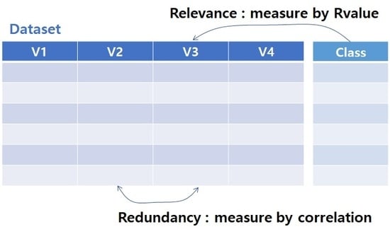
In this study, we propose new measures for redundancy and relevancy. We suggest Pearson’s correlation coefficient [16] as a redundancy measure and the R-value [17] as a relevance measure. The R-value and correlation coefficient can be designed for continuous variables whereas mutual information implies categorical variables. We also implement advanced mRMR (AmRMR) using new measures. Details of the new measures and AmRMR are provided in the next section.

2. Materials and Methods

2.1. Pearson’s Correlation Coefficient and R-Value

Pearson’s correlation coefficient is a measure of the linear correlation between two variables x and y, and it is defined by Equation (6):

$$\mathrm{r}=\frac{{\sum }_{i=1}^n\left(x_i-\overline{x}\right)\left(y_i-\overline{y}\right)}{\left(n-1\right)S_x{S}_y}=\frac{{\sum }_{i=1}^n\left(x_i-\overline{x}\right)\left(y_i-\overline{y}\right)}{\sqrt{{\sum }_{i=1}^n{\left(x_i-\overline{x}\right)}^2{\sum }_{i=1}^n{\left(y_i-\overline{y}\right)}^2}}$$

(6)

$$\overline{x}, \overline{y} :mean of x, y$$

$$S_x,S_y :standard deviation of x, y$$

It has a value range [−1, +1]. If an absolute value of the correlation coefficient is near 1, the variables (x, y) have strong correlation. In the context of feature selection, if two features (x, y) represent similar values, then the correlation coefficient of (x, y) will be high; this means that the correlation coefficient can be used to measure redundancy. If two features (a, b) have strong negative correlation, their values will be different. However, from the point of view of information theory, the amount of information in a and b is similar, and they can be considered redundant features.

The R-value is proposed as an evaluation measure for datasets [17,18]. The motivation for using the R-value is that the quality of the dataset has a profound effect on classification accuracy, and overlapping areas among classes in a dataset have a strong relationship that determines the quality of the dataset. For example, dataset D₁ produces higher classification accuracy than dataset D₂ in Figure 1. Overlapping area is a region where samples from different classes are gathered closely to one another. If an unknown sample is located in the overlapping area, it is difficult to determine its class label. Therefore, the size of overlapping areas may be a criterion to measure the quality of features or of the entire dataset [19]. The R-value captures overlapping areas among classes in a dataset. The R-value uses a k-nearest neighbor algorithm to define overlapping areas. If an instance has many neighbors that have different class values, then it may belong to an overlapping area. Suppose DS is a given dataset, S is a subset of features, and C is a class vector. Algorithm 2 describes the procedure to calculate the R-value of S. The R-value has range [0, 1], and if the R-value of S is near 1, then S may produce lower classification accuracy.

Algorithm 2:Rvalue(S,C)

//K: number of nearest neighbor

Derive dataset DSs of S from DS;

OV ← 0;         //

N ← number of instances of DSs[];

FOR each instance in DSs[i] DO

Find K nearest neighbor values for DSs[i] and store their instance ID to KNV;

Count the number of elements in KNV that have class value different from C[i], and add it to OV;

END FOR

Rvalue ← OV/(K*N);

RETURNRvalue;

2.2. Formal Description of AmRMR

Suppose we evaluate a feature set S that has m features. The new relevancy measure VR for S is simply defined using the Rvalue:

$$V_R=1-Rvalue\left(S,C\right)$$

(7)

If a feature set S produces a high Rvalue, it means that large overlapping areas exist between classes and may cause lower classification accuracy. Therefore, the lower the Rvalue obtained, the better the classification. We define the new relevancy measure as 1 − Rvalue to give a higher score to a lower Rvalue.

To develop a better redundancy measure, we replace mutual information with a correlation coefficient. The original redundancy measure, W_I, is simply the mean of the mutual information for a pair of features in S. From several experiments, we found that the value of a specific pair of features is more important than the mean of all pairs if the value is high. Therefore, we calculate a maximum (maxC) and a mean (meanC) of the correlation coefficient, and choose maxC as a new redundant measure W_R if maxC ≥ 0.5, otherwise W_R = meanC. If the absolute value of correlation coefficient of variables (x,y) ≥ 0.5, we accept that they have meaningful correlation. In Equations (8) and (9), Cor() is a correlation coefficient function, abs() is an absolute value function, and max() is a maximum value function.

$$\begin{gathered} max\mathrm{C}=\max \left\{\mathrm{abs}\left(\mathrm{Cor}\left(f_i,f_j\right)\right)\right\} \\ {f}_i,f_j\in S,i,j=1,2,3,\dots ,m \end{gathered}$$

(8)

$$\begin{gathered} mean\mathrm{C}=mean\left\{\mathrm{abs}\left(\mathrm{Cor}\left(f_i,f_j\right)\right)\right\} \\ {f}_i,f_j\in S,i,j=1,2,3,\dots ,m \end{gathered}$$

(9)

$$W_R=\{\begin{array}{c}maxC, if maxC \ge 0.5\\ meanC, if maxC< 0.5 \end{array}$$

(10)

From the new definition of relevance measure V_R and redundant measure W_R, we redefine MID and MIQ as RVD and RVQ, respectively. RVD is similar to MID. We define RVQ in a more sophisticated manner. In evaluation function RVQ, V_R indicates benefit and W_R indicates penalty. Therefore, (V_R/W_R) cannot be larger than V_R. However, 0 ≤ V_R, W_R ≤ 1 in our equation, and sometimes (V_R/W_R) > V_R. Therefore, we adjust for this discrepancy in Equation (12).

$$RVD=V_R-W_R$$

(11)

$$RVQ=\{\begin{array}{l}{V}_R,if \left(\frac{V_R}{W_R}\right)>V_R \\ \frac{VR}{WR},if \left(\frac{V_R}{W_R}\right)\le V_R \end{array}$$

(12)

We have described a new evaluation measure for feature subset S. As we mentioned earlier, we cannot evaluate all instances of S for a given dataset; thus, a heuristic approach is required. We implemented AmRMR based on mRMR code. It applies a forward search to reduce the search space. Algorithm 3 describes the pseudo code for AmRMR. We only consider the case of RVQ.

Algorithm 3: AmRMR(DS,C,M)

/*

DS: target dataset

C: class vector of DS

M: size of feature subset S that we want to get

F: set of features in DS

*/

Find fi ∈ F that produces max(R-value( fi,C));

S ← {fi};

Remove fi from F;

REPEAT UNTIL |S| < M

max_eval ← 0;

max_idx ← 0;

FOR each fj ∈ F DO

Target ← S ∪ {fi};

Calculate RVQ for Target;

IF RVQ > max_eval THEN

max_eval ← RVQ;

max_idx ← j;

END IF

END FOR

S ← S ∪{fmax_idx};

Remove fj from F;

END REPEAT

RETURNS;

3. Result

To compare mRMR and AmRMR algorithms, we collected several types of datasets that have different numbers of features, classes, and instances.

Table 1. Summary of benchmark datasets.

Dataset	Instances	Features	Classes
GDS2546	167	1000	4
GDS2547	164	1000	4
GDS3715	109	1000	4
Hill Valley	1212	100	2
Isolet	7797	617	26
Madelon	2000	500	2
Phoneme	4509	256	5
MLL	72	12533	3
Arcene	99	10001	2
Gisette	5999	5000	2

summarizes the datasets. We obtained GDS2546, GDS2547, and GDS3715 from the NCBI Gene Expression Omnibus [20], and arcene and madelon from NPIS2003’s challenge of feature selection [21], and others were obtained from the UCI Machine Learning Repository [22]. We took 5–25 features using mRMR and AmRMR, and performed classification tests using k-nearest neighbor (KNN), support vector machine (SVM), C5.0 (C50), and random forest (RF). To avoid an overfitting problem, we adopted a k-fold cross-validation, where k is 10. In the case of arcene and madelon, we took feature set from the training dataset and performed classification tests using validation datasets because they support separated training/validation datasets.

Table 2. Summary of classification accuracy tested by KNN.

Dataset		Number of Features
		5	10	15	20	25
GDS2546	mRMR	0.623	0.647	0.628	0.598	0.628
	AmRMR	0.695	0.719	0.719	0.719	0.719
GDS2547	mRMR	0.598	0.610	0.628	0.634	0.653
	AmRMR	0.726	0.762	0.744	0.762	0.793
GDS3715	mRMR	0.780	0.79	0.808	0.770	0.798
	AmRMR	0.89	0.936	0.964	0.936	0.955
Hill Valley	mRMR	0.546	0.553	0.542	0.549	0.557
	AmRMR	0.601	0.609	0.6	0.605	0.612
Isolet	mRMR	0.374	0.56	0.607	0.688	0.713
	AmRMR	0.528	0.756	0.830	0.875	0.893
Madelon	mRMR	0.702	0.824	0.83	0.819	0.8
	AmRMR	0.866	0.894	0.895	0.896	0.896
Phoneme	mRMR	0.830	0.857	0.863	0.879	0.895
	AmRMR	0.884	0.916	0.921	0.922	0.925
MLL	mRMR	0.941	0.821	0.906	0.917	0.930
	AmRMR	1	1	1	1	1
Arcene	mRMR	0.52	0.58	0.56	0.66	0.65
	AmRMR	0.79	0.79	0.82	0.81	0.82
Gisette	mRMR	0.608	0.67	0.79	0.828	0.825
	AmRMR	0.886	0.9	0.9	0.901	0.901

,

Table 3. Summary of classification accuracy tested by SVM.

Dataset		Number of Features
		5	10	15	20	25
GDS2546	mRMR	0.677	0.736	0.688	0.677	0.695
	AmRMR	0.652	0.647	0.706	0.743	0.713
GDS2547	mRMR	0.701	0.652	0.681	0.695	0.689
	AmRMR	0.701	0.701	0.738	0.739	0.719
GDS3715	mRMR	0.79	0.771	0.771	0.808	0.789
	AmRMR	0.853	0.899	0.908	0.899	0.890
Hill Valley	mRMR	0.518	0.516	0.516	0.52	0.52
	AmRMR	0.526	0.527	0.529	0.525	0.526
Isolet	mRMR	0.382	0.603	0.667	0.741	0.775
	AmRMR	0.556	0.793	0.870	0.902	0.919
Madelon	mRMR	0.719	0.714	0.696	0.678	0.674
	AmRMR	0.829	0.81	0.752	0.705	0.685
Phoneme	mRMR	0.848	0.866	0.872	0.889	0.905
	AmRMR	0.895	0.923	0.928	0.927	0.932
MLL	mRMR	0.899	0.899	0.942	0.957	0.942
	AmRMR	0.971	0.957	0.971	0.985	0.958
Arcene	mRMR	0.719	0.714	0.696	0.678	0.674
	AmRMR	0.829	0.81	0.752	0.705	0.685
Gisette	mRMR	0.848	0.866	0.872	0.889	0.905
	AmRMR	0.895	0.923	0.928	0.927	0.932

,

Table 4. Summary of classification accuracy tested by C50.

Dataset		Number of Features
		5	10	15	20	25
GDS2546	mRMR	0.612	0.653	0.641	0.641	0.628
	AmRMR	0.653	0.611	0.664	0.623	0.658
GDS2547	mRMR	0.537	0.512	0.591	0.598	0.659
	AmRMR	0.622	0.634	0.628	0.677	0.640
GDS3715	mRMR	0.798	0.743	0.771	0.733	0.689
	AmRMR	0.752	0.752	0.752	0.764	0.754
Hill Valley	mRMR	0.475	0.475	0.475	0.475	0.475
	AmRMR	0.475	0.475	0.475	0.475	0.475
Isolet	mRMR	0.388	0.566	0.609	0.684	0.750
	AmRMR	0.511	0.715	0.769	0.805	0.815
Madelon	mRMR	0.693	0.712	0.720	0.729	0.743
	AmRMR	0.741	0.807	0.804	0.786	0.786
Phoneme	mRMR	0.815	0.825	0.830	0.843	0.878
	AmRMR	0.876	0.898	0.889	0.888	0.884
MLL	mRMR	0.845	0.818	0.804	0.901	0.800
	AmRMR	0.859	0.859	0.859	0.859	0.830
Arcene	mRMR	0.690	0.830	0.840	0.820	0.800
	AmRMR	0.780	0.860	0.860	0.820	0.830
Gisette	mRMR	0.849	0.854	0.866	0.882	0.904
	AmRMR	0.916	0.943	0.949	0.947	0.949

and

Table 5. Summary of classification accuracy tested by Random Forest (RF).

Dataset		Number of Features
		5	10	15	20	25
GDS2546	mRMR	0.653	0.737	0.761	0.755	0.744
	AmRMR	0.629	0.665	0.731	0.742	0.713
GDS2547	mRMR	0.677	0.658	0.652	0.683	0.695
	AmRMR	0.744	0.780	0.762	0.750	0.768
GDS3715	mRMR	0.844	0.799	0.835	0.808	0.817
	AmRMR	0.872	0.890	0.890	0.900	0.890
Hill Valley	mRMR	0.543	0.556	0.560	0.582	0.583
	AmRMR	0.626	0.648	0.643	0.640	0.637
Isolet	mRMR	0.412	0.627	0.682	0.760	0.790
	AmRMR	0.556	0.798	0.868	0.898	0.911
Madelon	mRMR	0.754	0.789	0.794	0.791	0.772
	AmRMR	0.849	0.861	0.848	0.840	0.832
Phoneme	mRMR	0.846	0.864	0.874	0.890	0.902
	AmRMR	0.893	0.917	0.920	0.924	0.926
MLL	mRMR	0.958	0.986	0.971	0.971	0.971
	AmRMR	0.986	0.986	0.971	1.000	0.956
Arcene	mRMR	0.790	0.900	0.870	0.840	0.820
	AmRMR	0.890	0.900	0.900	0.880	0.880
Gisette	mRMR	0.857	0.867	0.884	0.900	0.921
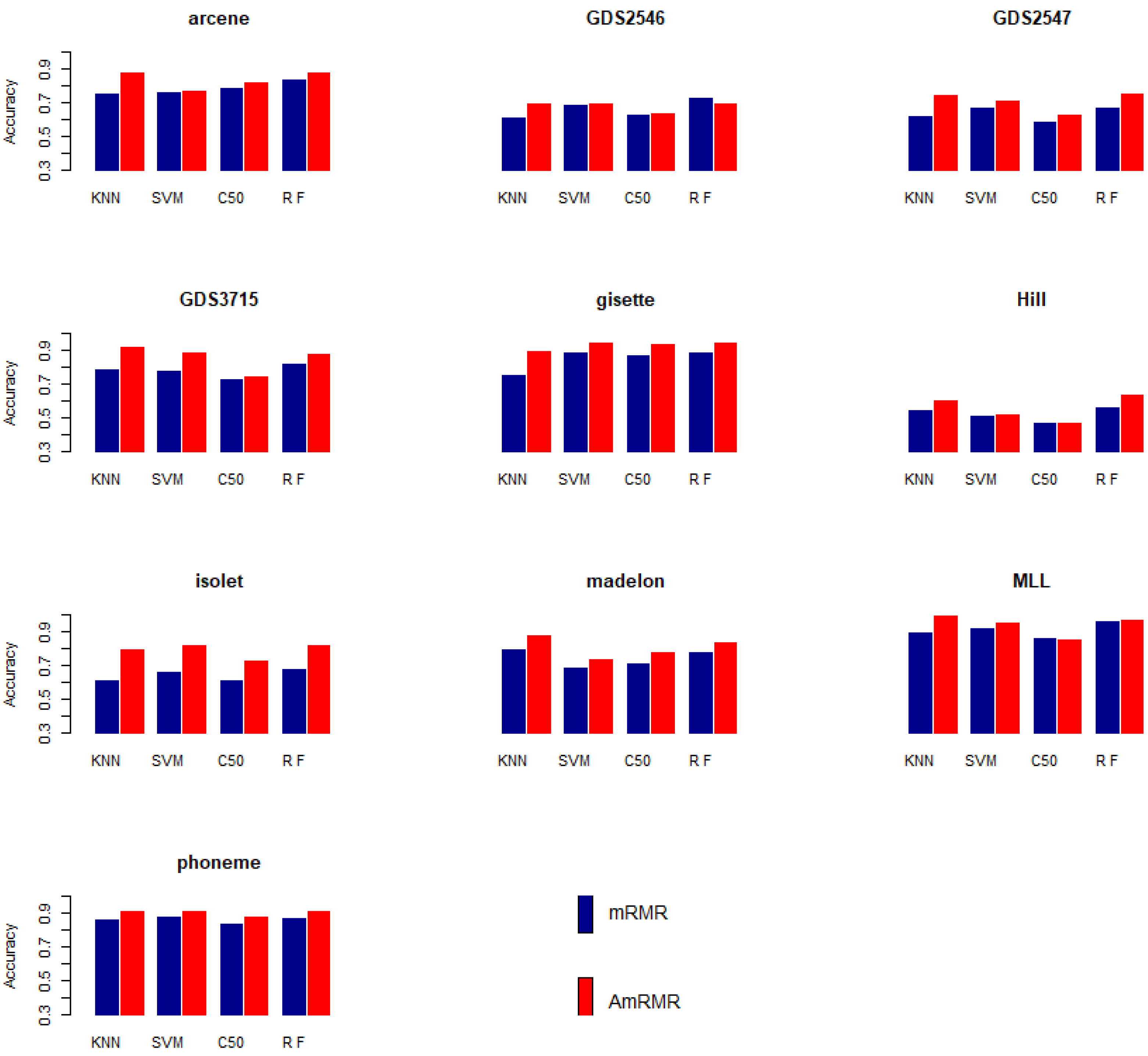
	AmRMR	0.918	0.948	0.961	0.964	0.967

summarize the results. In most of the cases, AmRMR produces better performance than mRMR. Figure 2 summarizes the classification results in Table 2, Table 3, Table 4 and Table 5. Each accuracy means average classification accuracy from 5 to 25 features of datasets. Each graph clearly shows AmRMR chooses better features than mRMR.

4. Discussion

In general, the R-value is better than mutual information as a measure of relevance between features and class vector. Mutual information is a statistical measure and it needs categorical values to calculate probability. Therefore, if a target dataset contains continuous values, we need to discretize them before applying mRMR. Information loss is inevitable in discretization. The R-value does not need discretization and is more advantageous than mutual information when a dataset has continuous values. Another weak point of mutual information is that it can calculate I(f_i, C) where f_i is a feature and C is a class vector, but it cannot calculate I({f₁, f₂, f₃}, C) because it is based on probability. Therefore, it uses (I(f₁, C) + I(f₂, C) + I(f₃, C))/3 to calculate relevance between {f₁, f₂, f₃} and C. This calculation cannot fully capture interactions among {f₁, f₂, f₃}. In contrast, the R-value is a dimensionless distance-based measure so R-value({f₁, f₂, f₃}, C) can be directly calculated.

mRMR and AmRMR output different feature sets from the same dataset, resulting in different classification accuracies.

Table 6. List of features selected by mRMR and AmRMR.

Dataset		Selected Feature’s ID
GDS3715	mRMR	1, 510, 4, 153, 48, 84, 2, 5, 516, 6, 32, 19, 700, 662, 270, 240, 9, 450, 129, 122, 25, 7, 29, 238, 12
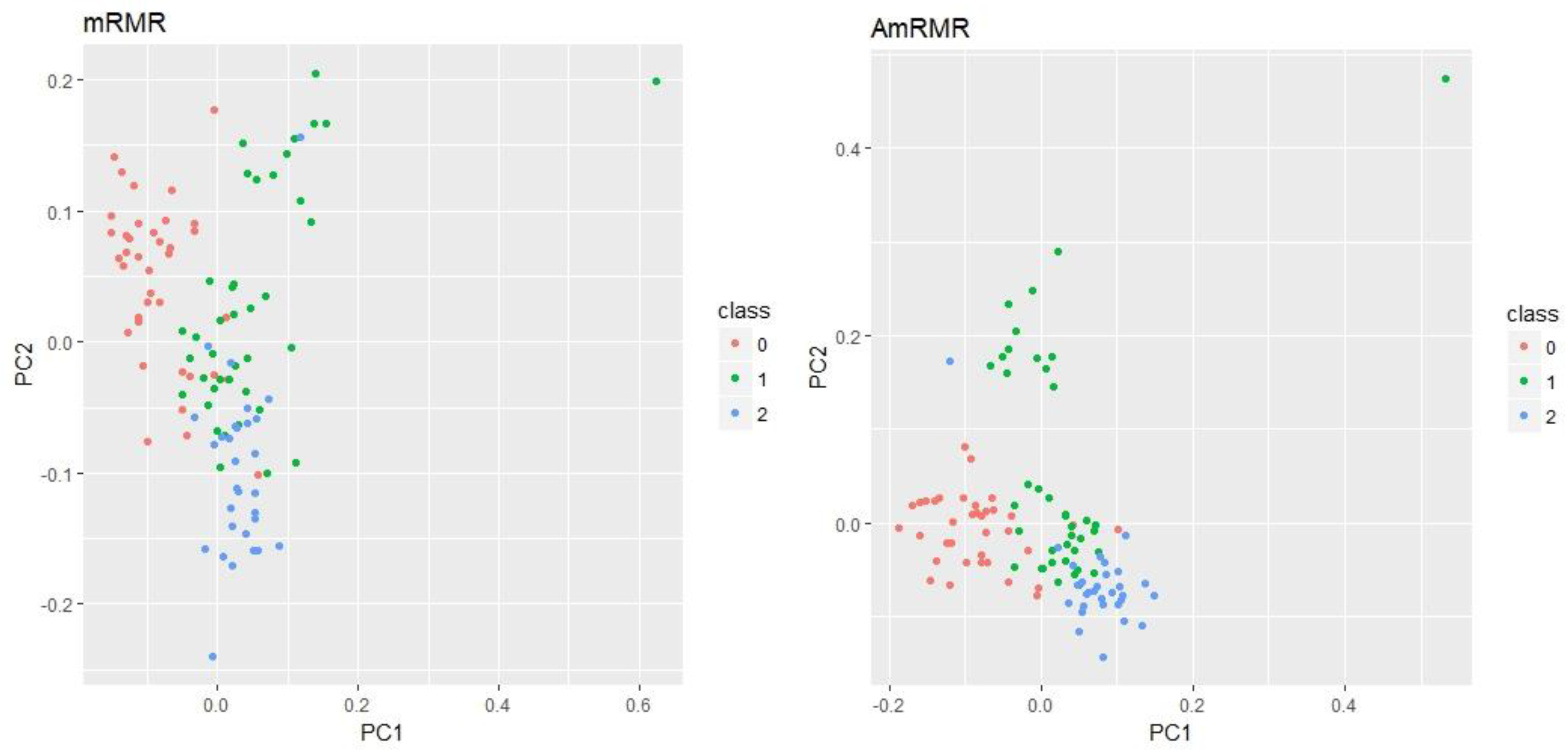
	AmRMR	25, 269, 132, 90, 15, 108, 577, 301, 121, 991, 167, 273, 334, 661, 447, 19, 873, 210, 583, 26, 751, 248, 197, 558, 215

shows a list of 25 features from GDS3715 dataset evaluated by mRMR and AmRMR. In the case of Arcene, there is only one shared feature (9970) between mRMR and AmRMR. In the case of Madelon, there are five shared features. It means that mRMR and AmRMR have different evaluation criteria for feature selection. Figure 3 shows PCA (Principal Component Analysis) plots for Arcene and Madelon using five features by mRMR and AmRMR. As we can see, PCA plots of AmRMR show a clearer distribution of class instances than mRMR. It explains why the feature set of AmRMR produces better classification accuracy than the one used by mRMR.

Table 7. Improved classification accuracy by AmRMR.

Classifier	Number of features					Average
	5	10	15	20	25
KNN	0.100	0.116	0.108	0.108	0.102	0.107
SVM	0.056	0.063	0.071	0.058	0.044	0.058
C50	0.048	0.057	0.050	0.034	0.030	0.044
RF	0.046	0.043	0.045	0.044	0.036	0.043

shows averages of the improved classification accuracy for 10 datasets. In the four classifiers, 4–10% of accuracies are improved. This result indicates that the proposed new redundancy and relevance measures enhance performance compared to the original mRMR measures. KNN classifier shows remarkably improved result (10.7%). The reason is in the R-value, which is a measure of relevance. Both KNN and R-value are based on k-nearest neighbor. Therefore, a set of features with good R-value may produce good classification accuracy by KNN. The relationship between R-value and KNN is similar to the relationship between the classifier and the feature evaluation measure in the wrapper method.

The proposed new redundancy and relevance measures are tailored to datasets that have continuous values. This means that they are not suitable for datasets that have categorical values. The mutual information measure in the original mRMR method is more suitable for categorical datasets. Nevertheless, AmRMR is useful, because there exist many high-dimensional continuous datasets such as microarray data, diagnosed diseases data, image analysis data, and so on.

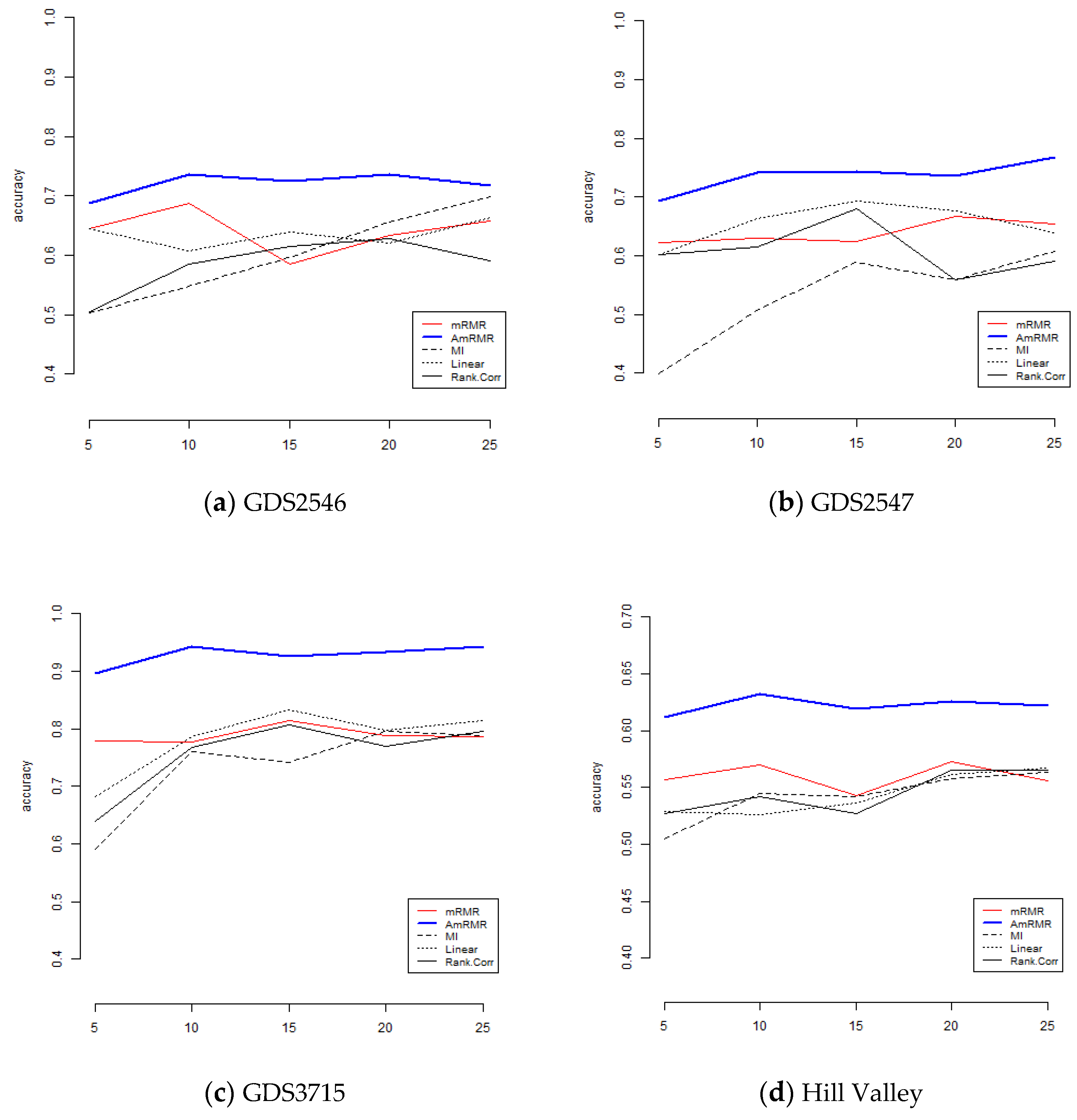
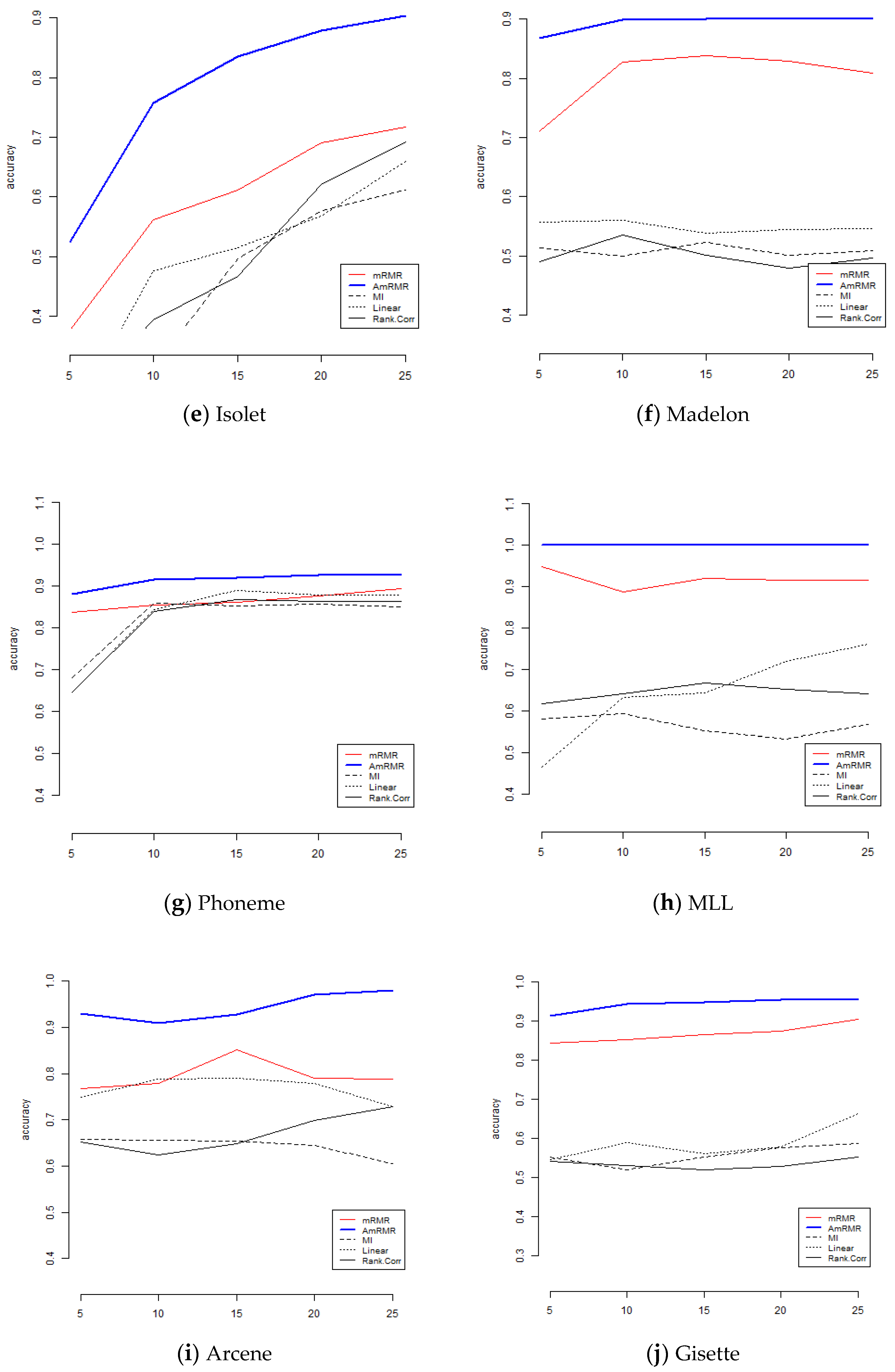
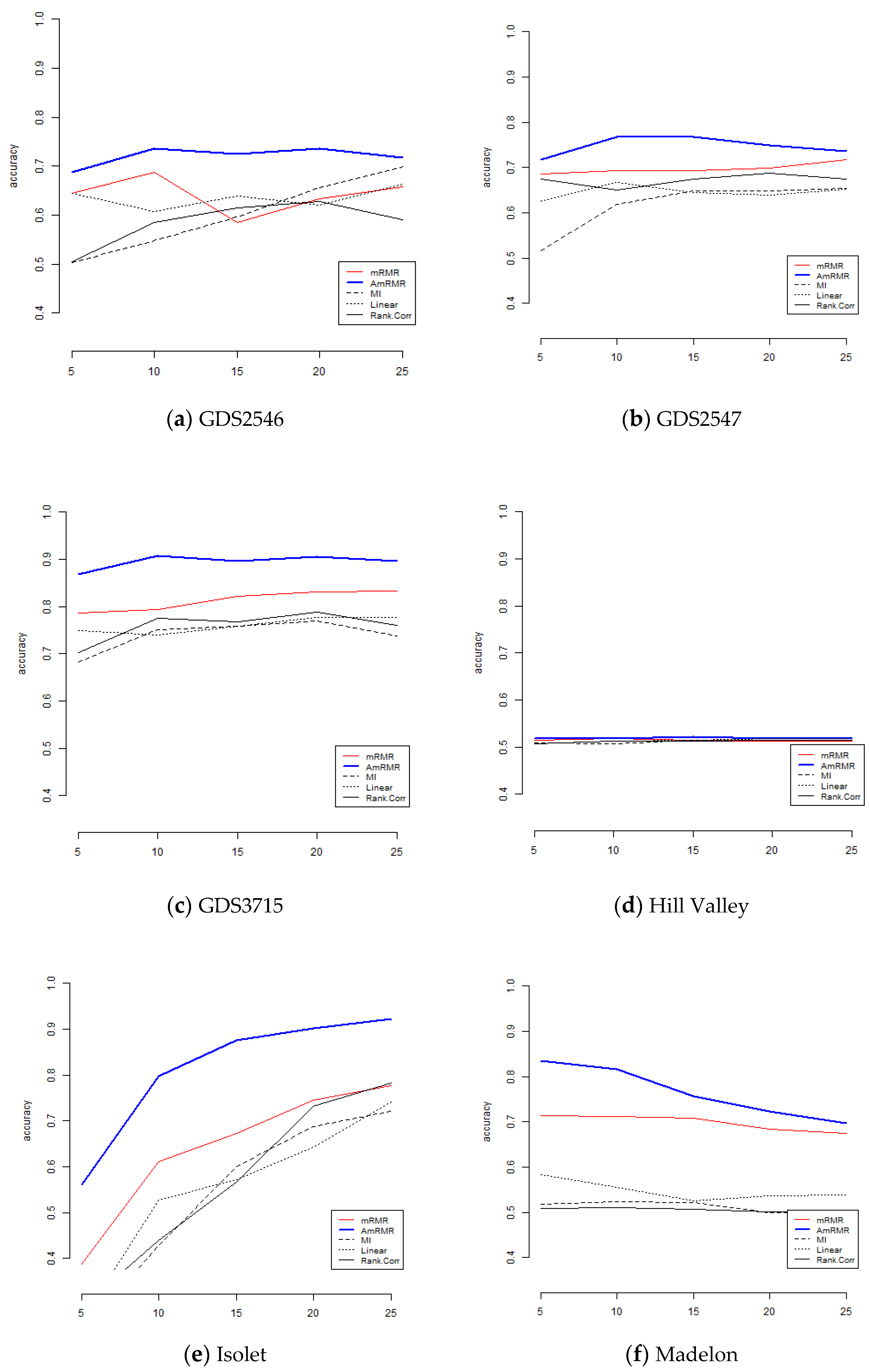
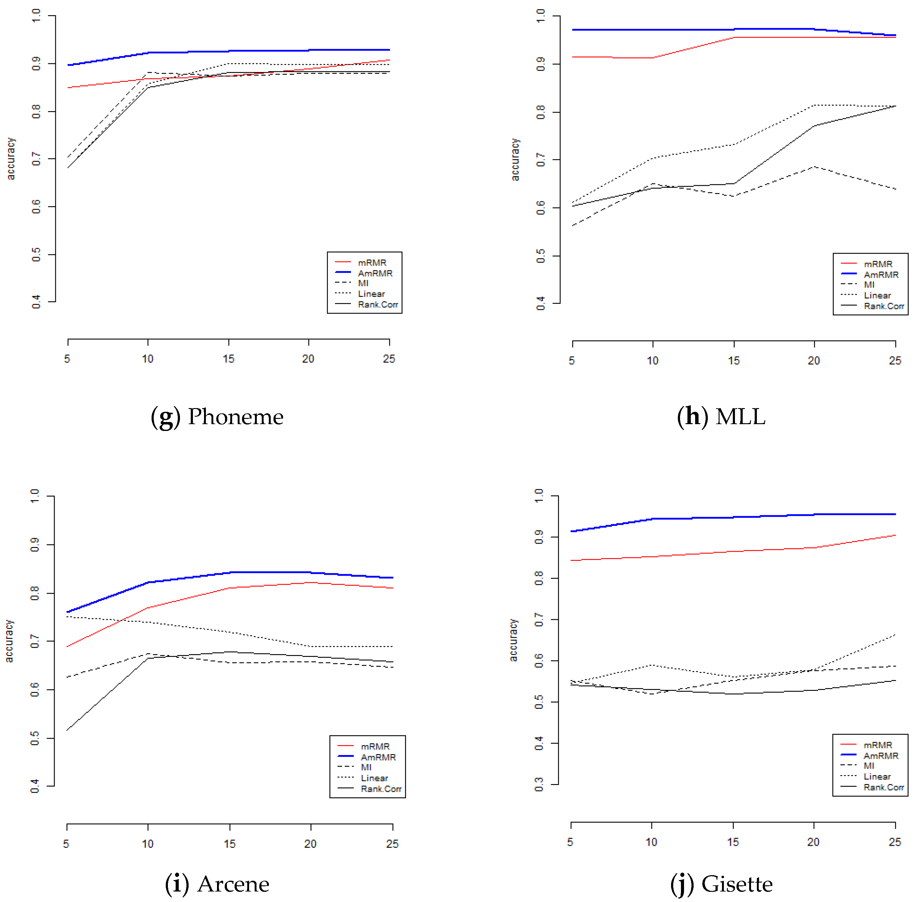
To show the effect of AmRMR, we compare it with three filter feature selection methods such as mutual information (MI), linear correlation (Linear), and rank correlation (Rank.Corr). The condition of comparison is the same as for the case of mRMR. For simplicity, we test KNN and SVM. Figure 4 and Figure 5 are the results of comparison. We can see AmRMR produces the highest performance of all the methods.

5. Conclusions

In this study, we proposed new redundancy and relevance measures to improve mRMR feature selection. The proposed method provides powerful performance for specific target dataset than mRMR. However, it should be noted that the proposed method has its limitations on types of datasets it can analyze. The performance of feature selection depends on the characteristics of the target dataset. Therefore, users are encouraged to test both mRMR and AmRMR, and choose the better feature subsets according to the test results. The entire set of R codes for AmRMR is available at https://bitldku.github.io/home/sw/AmRMR.html.