Article

Sentiment Analysis of Lithuanian Texts Using Traditional and Deep Learning Approaches

by
Jurgita Kapočiūtė-Dzikienė
1,*,
Robertas Damaševičius
2 and
Marcin Woźniak
3
1
Faculty of Informatics, Vytautas Magnus University, K. Donelaičio 58, 44248 Kaunas, Lithuania
2
Department of Software Engineering, Kaunas University of Technology, K. Donelaičio 73, 44249 Kaunas, Lithuania
3
Institute of Mathematics, Silesian University of Technology, Kaszubska 23, 44-100 Gliwice, Poland
*
Author to whom correspondence should be addressed.
Computers 2019, 8(1), 4; https://doi.org/10.3390/computers8010004
Submission received: 27 November 2018 / Revised: 21 December 2018 / Accepted: 24 December 2018 / Published: 1 January 2019

Abstract

:
We describe the sentiment analysis experiments that were performed on the Lithuanian Internet comment dataset using traditional machine learning (Naïve Bayes Multinomial—NBM and Support Vector Machine—SVM) and deep learning (Long Short-Term Memory—LSTM and Convolutional Neural Network—CNN) approaches. The traditional machine learning techniques were used with the features based on the lexical, morphological, and character information. The deep learning approaches were applied on the top of two types of word embeddings (Vord2Vec continuous bag-of-words with negative sampling and FastText). Both traditional and deep learning approaches had to solve the positive/negative/neutral sentiment classification task on the balanced and full dataset versions. The best deep learning results (reaching 0.706 of accuracy) were achieved on the full dataset with CNN applied on top of the FastText embeddings, replaced emoticons, and eliminated diacritics. The traditional machine learning approaches demonstrated the best performance (0.735 of accuracy) on the full dataset with the NBM method, replaced emoticons, restored diacritics, and lemma unigrams as features. Although traditional machine learning approaches were superior when compared to the deep learning methods; deep learning demonstrated good results when applied on the small datasets.

1. Introduction

Internet has changed the ways how people express their beliefs and sentiments about products or services, events, topics, interactions, etc. It is mainly done via social networks, review websites, web forums, blogs, and Internet comments. These texts are sentiment rich, and are therefore beneficial for companies or individuals willing to improve their product marketing strategies and respond accordingly. Methods of automatic sentiment analysis are commonly chosen for this purpose. Sentiment analysis has been used for analyzing sentiments of tweets on health topics [1], evaluate teachers ability and predict student performance [2], identify contextual polarity of drugs, movie, and restaurant reviews [3,4,5], examine public opinion on products and services and societal issues [6], classify e-learners and their topics of interest in their social networks interactions [7], perform opinion mining in tweets [8,9], analyze sentiment orientation of microblogs [10], and forecast stock prices from sentiments of news signals in the financial markets [11].
Sentiment analysis (or classification) methods can be grouped into two main categories: dictionary-based and machine learning. The dictionary-based methods (such as [12,13,14,15]) typically rely on the external lexical resources of sentiment words and syntactic–semantic knowledge. Unfortunately, but such resources (as, e.g., SentiWordNet (SentiWordNet is a WordNet with the positive, negative, and neutral values assigned to each synset (more about SentiWordNet is in https://sentiwordnet.isti.cnr.it/))) are not available for the lower resourced languages.
An alternative for the dictionary-based methods are machine learning methods (see [16,17]), such as Support Vector Machines (SVM), Naïve Bayes Multinomial (NBM), and k-Nearest Neighbors (kNN). These methods are typically applied on (weighted) frequency-based features (e.g., lexical, character, morphological, etc.).
Recently, the deep learning methods (which also belong to the group of machine learning) have gained interest in many text classification tasks, including sentiment analysis. As claimed in [18], a Deep Neural Network (DNN) architecture that jointly uses character-, word-, and sentence- level representations achieves state-of-the-art performance for binary (positive and negative) classification on the Stanford Sentiment Treebank of movie reviews [19] and the Stanford Twitter sentiment corpus [20]. Katoh and Ninomiya in [21] solve the binary sentiment classification task on the English and Japanese datasets. The authors prove that multi-layer Neural Networks (NNs) work well only on large-scale datasets, but for smaller datasets NNs without hidden layers are more suitable. The Convolutional Neural Network (CNN) has been applied on the binary-class Twitter dataset used as the benchmark in the SemEval-2015 competition [22]. The experiments that are described in [23] are performed on the English binary review data obtained from Amazon. Authors used the CNN method with Google News word2vec embeddings and demonstrated superiority over the baseline methods. A hybrid approach applied on the Hindi language and the dataset of four classes (positive, negative, neutral, and conflict) is based on the CNN architecture augmented with a set of optimized features selected through the multi-objective optimization framework. Subsequently, the augmented optimization vector is used for training the SVM [24]. Yousif et al. [25] used a hybrid neural model, which combines CNN and Recurrent NN (RNN) to capture local n-gram features and long-term dependencies of the text for classification of sentiments and purposes of scientific citations. Yun et al. [26] combined with the vector space and CNN methods. Firstly, they select the words that are based on the spatial distribution of features in text information and map these words into abstract vectors based on the dictionary. Afterwards, CNN is used to extract features of abstract vectors for sentiment classification.
Stojanovski et al. in [27] used CNN and RNN to obtain more diverse representations on a top of GloVe (Global Vectors) word embeddings. For texts of the variable length, CNN and RNN allow to extract fixed length representation vectors and to use their concatenation. Their result applied on the binary or five classes (positive, negative, neutral, very positive, very negative) benchmark Twitter datasets, was ranked the second best in the SemEval-2016 task [27]. Lu et al. [28] compared RNN and CNN trained on neural embeddings with SVM trained on unigram, bigram, and unigram + bigram features. They results showed that deep learning methods underperformed in most of the SVM models on English and Japanese sentiment datasets with either two or three classes. Cortis et al. [29] summarized sentiment analysis works that were presented by 32 participants in the SemEval-2017 Task 5 on the Financial Microblogs and News data. The traditional machine learning based technique (rather than deep learning) was ranked as the first: it employed linguistic, sentiment lexicon, domain-specific features, and Google word embeddings to construct models of ensemble regression algorithms [30]. The second best technique was based on deep learning, i.e., an ensemble-based model that combined CNN with Long Short-Term Memory (LSTM) and word embeddings [31]. The competition of in the SemEval-2017 Task 4 that is described in [32] attracted 48 teams. Sentiment analysis was done on the Twitter data of two or five classes. The best-ranked teams used deep learning: e.g., BB_twtr employed an ensemble of LSTM and CNN methods with multiple convolution operations [33]; and, DataStories applied LSTM network with attention mechanism [34].
Although the results of sentiment analysis are mixed (i.e., there is no consensus which method is the best), deep learning has become the dominant paradigm recently. Due to this reason in this research, we also investigate an impact of the deep learning approaches for the sentiment analysis task. Here, we deal with the dataset of Lithuanian Internet comments containing three classes (positive, negative, and neutral) by testing two deep learning approaches (LSTM and CNN with two types of neural word embeddings). However, the deep learning approaches are effective only on the large training datasets and when applied on the top of the comprehensive list of word embeddings (trained from huge text corpora), therefore they may not be effective on the Lithuanian datasets for our solving task. Due to this reason for the comparison purposes, we test two traditional machine learning approaches (SVM and NBM with five types of feature representations) and evaluate an impact of pre-processing techniques (replacement of emoticons with sentiment words, removal of stop words, elimination/restoration of diacritics) and dataset sizes (full and balanced). Unfortunately, we cannot compare machine learning approaches with the dictionary-based because important lexical resources (e.g., SentiWordNet) either do not exist for the Lithuanian language or are too small to achieve reasonable results (some previous attempts to tackle the sentiment analysis task for the Lithuanian language based on the sentiment lexicon were not very successful [35]). Thus, the main purpose of this research is to test various machine learning methods (their parameters, pre-processing techniques), to compare the results, and to offer the best solution for the sentiment classification of non-normative Lithuanian texts.

2. Methodology

2.1. Formal Definition of the Task

The sentiment classification task in our research can be interpreted as the supervised text classification task.
Let d 1 , d 2 ,   , d n be the texts (Internet comments) attached to only one of c 1 , c 2 ,   , c m class (where m = 3, because we have positive, negative, and neutral sentiments). Hence, our solving task is a single-label but multi-class (m > 2) classification problem.
Let function γ denote a mapping of texts to their sentiments (i.e., classes): γ : D C . A goal is to choose a method that could find the best approximation of γ . For this reason, we have compared two groups of methods: i.e., traditional machine learning techniques with discrete representations (described in Section 2.3) and deep learning methods with distributional representations (described in Section 2.4).

2.2. The Dataset

We used the dataset of the Lithuanian Internet comments (see Table 1). Texts in this dataset were labeled with positive, negative, and neutral polarities by two human-experts based on their mutual agreement (i.e., experts assessed comments independently and only the texts that obtained the same polarity values were included into the dataset). The dataset is of the general domain: it contains opinions about articles on the various topics (politics, sport, health, economics, etc.) presented in the Lietuvos Rytas news portal https://www.lrytas.lt/ and crawled in March, 2013. The Internet comments represent the non-normative Lithuanian language.
The Lithuanian language is vocabulary rich (the Dictionary of Lithuanian [36] contains more than 0.5 million headwords, whereas the Oxford English Dictionary [37] contains ~0.35 million); fusional and morphologically complex; derivationally rich (e.g., verbs can be made from the onomatopoeias, it also has ~60 prefixes and ~600 suffixes [38], some of which are used to derivate diminutives and hypocoristic words). The diminutives and hypocoristic words—which are very common in the spoken language (e.g., the word dukra (daughter) can be found as dukrytė, dukružytė, etc.)—can have more than one suffix, and in some rare cases their number increase up to six. Moreover, the non-normative Lithuanian language has one more problem in that English does not confront, i.e., word diacritics. In the non-normative Lithuanian texts word diacritics are used or omitted based on the author’s choice. Words with omitted diacritics either become out-of-vocabulary words or (in most of the cases) obtain absolutely different meaning, which is ambiguous (e.g., karštas (hot) and karstas (coffin)), and even hold the opposite sentiment polarity. Besides undiacritized words, the non-normative Lithuanian texts contain other out-of-vocabulary words (including foreign language inserts, words with the spelling errors, jargon, abbreviations, etc.), emoticons, etc.
The second version of the dataset (presented in Table 2) in each category contains an equal number of texts, which were randomly selected from the “main pool” (i.e., from the dataset presented in Table 1). The detailed description about this version of the dataset can be found in [35].
Despite the non-normative texts being rather noisy (e.g., have missing diacritics), they may contain some valuable information (e.g., emoticons), which, if taken into account can facilitate the solving task. Due to this and previously mentioned reasons about the non-normative Lithuanian language specifics, we have explored the impact of the following pre-processing techniques:
  • No pre-processing. The texts were lowercased, numbers and punctuation were eliminated.
  • With emoticons. As proved in [39], the emoticon replacement assures the higher classification accuracy. In our experiments we have used 32 groups of emoticons, where each group was mapped into the appropriate sentiment word (presented in its main vocabulary form). For instance, all the emoticons of this group “:(”, “:-(”, “:-c”, “:-[”, etc. have the same meaning liūdnas (sad) and therefore can be replaced with liūdnas in the text. When using this pre-processing technique, all of the words were lowercased; the detected emoticons were replaced with the appropriate sentiment words; numbers and punctuation were eliminated.
  • No stop words. Intuitively, such words as acronyms, conjunctions or pronouns appear too often in all types of texts and are too short to carry important sentiment information. However, Spences and Uchyigit in [40] claim that interjections are strong indicators of subjectivity. Due to it, we have used a list of 555 stop words that does not contain interjections. During this text pre-processing step all words were lowercased and stop words, numbers, and punctuation were eliminated.
  • Diacritics elimination. The Lithuanian language uses the Latin alphabet supplemented with these diacritics: ą, č, ę, ė, š, ų, ū, ž. However, diacritics in the non-normative Lithuanian texts are sometimes omitted, therefore the same word in the non-normative texts can be found in both cases, i.e., written with or without diacritics. It causes ambiguity problems and increases the data sparseness, which, in turn, negatively affects the accuracy. One of the solutions for decreasing the data sparseness is to distort the data by replacing diacritized letters with their American Standard Code for Information Interchange (ASCII ) equivalent symbols. However, such distortion may cause even more ambiguity problems, which in turn may degrade the performance. Hence, the diacritics elimination is a questionable pre-processing technique, where the effectiveness has to be tested experimentally. Using this pre-processing technique, the words were undiacritized, lowercased and numbers and punctuation were eliminated.
  • Diacritics restoration is another direction for decreasing the data sparseness and increasing the text quality. For this purpose, we were using the language modeling method (described in [41]), which was proved to be the best for the Lithuanian diacritization problems. This language modeling method used the bi-gram back-off strategy (having ~58.1 million bigrams and ~2.3 million unigrams) to restore diacritics in our non-normative texts. After diacritization, the words were lowercased and numbers and punctuation were eliminated.

2.3. Traditional Machine Learning Techniques

We have used two traditional machine learning approaches:
  • Support Vector Machine (SVM) [42] is a discriminative instance-based method, which for the very long time has been the most popular text classification technique. SVM can efficiently cope with the high dimensional feature spaces (e.g., without the feature selection, SVM has to handle ~26 K different features (see a number of distinct tokens in Table 1)); sparseness of the feature vectors (only ~9 words per text); and, it does not perform aggressive feature selection (i.e., does not lose potentially relevant information, which is important not to degrade the accuracy [43]).
  • Naïve Bayes Multinomial (NBM) [44] is a generative profile-based approach, which can also outperform popular SVM in the sentiment analysis tasks [16]. It is a simple, but rather fast technique, which performs especially well on a large number of features with equal significance. Besides, this method does not require huge resources for the data storage and it is often selected as a baseline approach.
We have used SMO (for the SVM) with the polynomial kernel and NBM implementations in the Weka (Hall et al., 2009) machine learning toolkit, version 3.6 (Weka machine learning toolkit can be found at http://www.cs.waikato.ac.nz/ml/weka/). All other parameters were set to their default values. Both the SVM and NBM methods were applied on a set of features generalizing different levels of abstraction:
  • Lexical. The token unigrams (a common bag-of-words approach) and both token bigrams + unigrams were extracted from the texts.
  • Morphological. These feature types cover unigrams of lemmas and bigrams + unigrams of lemmas. Before feature extraction, the texts had to be lemmatized. For the lemmatization we have used the Lithuanian morphological analyzer-lemmatizer Lemuoklis [45]. Lemuoklis can solve ambiguity problems and transform recognized words into their dictionary form. However, it is only effective on the normative texts, which basically means that all undiacritized, abbreviated, or slang words remain untouched.
  • Character. This feature type represents document-level character tetra-grams. Such n = 4 was selected because it demonstrated the best performance over the different n values on the Lithuanian language in the topic classification task [46].

2.4. Deep Learning Methods

We have used two deep learning approaches:
  • Long Short-Term Memory (LSTM) method [47] is a special type of the artificial neural network. This method analyzes the text word-by-word and stores the captured semantics in the hidden layers. Besides, its main advantage from the recurrent neural networks is that LSTM does not suffer from the vanishing gradient problem when learning long-term dependencies.
  • Convolutional Neural Network (CNN) [48] (presented in detail for the text classification in [49]) is a feed-forward artificial neural network (ANN) that contains one or more convolutional layers and the max-pooling. Convolutional layers help the method to go deeper by decreasing the number of parameters and the max-pooling layer helps to effectively determine discriminative phrases in the text. However, the size of the filters in each convolutional layer still remains an issue: too small windows may cause a loss of important information; too large windows may produce an enormous number of parameters.
For testing LSTM [50] and CNN [49], we have used their implementations in deeplearning4j [51]—the open-source distributed deep learning library for the Java Virtual Machine. However, the existing implementations could solve only binary classification tasks, therefore necessary adjustments to multi-class classification were performed by the authors of this research. Both methods truncate the texts exceeding 256 words (it is more than enough, because an average text length does not exceed 10 tokens), all other parameters were set to their default values.
Both deep learning methods were applied on distributional feature vectors presented as the neural word embeddings. In our experiments, we have used two types of embeddings:
  • Word2Vec. These embeddings were generated with the same deeplearning4j software, the continuous bag-of-words (CBOW) with the negative sampling and 300 dimensions. Under this architecture, a neural network had to predict a focus word by feeding its context words from the surrounding window (the detailed explanation of the method is in [52,53]). Using the corpus of ~234 million running words, it resulted in 687,947 neural word embeddings for the Lithuanian language (more about it can be found in [54]).
  • FastText [55]. It is an extension of Word2Vec that is offered by Facebook AI Research Lab. Instead of inputting the whole words into the network (as in Word2Vec case), each word (e.g., network) is split into several word-level character n-grams (netw, etwo, twor, work); the separate vectors are trained for all of these n-grams; and, are then summed to get a single vector for the whole word (network). In our experiments we have used two-million available Lithuanian FastText word embeddings. (The FastText Lithuanian word embeddings were downloaded from https://fasttext.cc/docs/en/crawl-vectors.html).
FastText embeddings were trained on various types of texts, because they contain both diacritized (e.g., gražus (beautiful), šaunus (cool), etc.) and undiacritized (grazus, saunus, etc.) versions of the same word. On the contrary, Word2Vec embeddings were trained on the normative Lithuanian texts only; therefore, intuitively they cannot be effective on the undiacritized texts (especially after the applied diacritics elimination pre-processing technique, as described in Section 2.2). Undiacritized non-normative texts are already distorted texts, therefore one of the solutions to find more matches among the word embeddings is to distort them the same way by removing diacritics. Such removal may cause disambiguation problems (because undiacritized version of some word can also exist in the normative Lithuanian language, but have the different form, meaning, or even different sentimental polarity), e.g., mama (mother in nominative) and mamą (mother in accusative), karstas (coffin), and karštas (hot). The list of embeddings cannot contain the word duplicates: if diacritics elimination caused some ambiguity, all embeddings of less frequent words were discarded from the list (e.g., karštas is more often than karstas, therefore karstas is eliminated from the list of word embeddings, and karštas replaced with undiacritized karstas). As the result, the total number of words embeddings dropped from 687,947 to 632,435 undiacritized word embeddings. Despite that such distortion may cause the accuracy degrade problems, we are still curious to see the impact on the results.

3. Experimental Set-Up and Results

The experiments were carried out on two datasets and different pre-processing techniques (described in Section 2.2) using either the traditional machine learning (presented in Section 2.3) or deep learning (described in Section 2.4) approaches. All of the experiments were performed using stratified 10-fold cross validation and were evaluated using macro-accuracy and f-score (averaged over classes and folds) performance measures [56].
We have also evaluated random (see Equation (1)) and majority (Equation (2)) baselines, because the results are considered as reasonable, if the accuracy values exceed random and majority baselines.
b a s e l i n e r a n d o m = P ( c i ) 2 ,   where   P ( c i )   is   the   probability   of   a   class   c i
b a s e l i n e m a j o r i t y = max ( P ( c i ) )
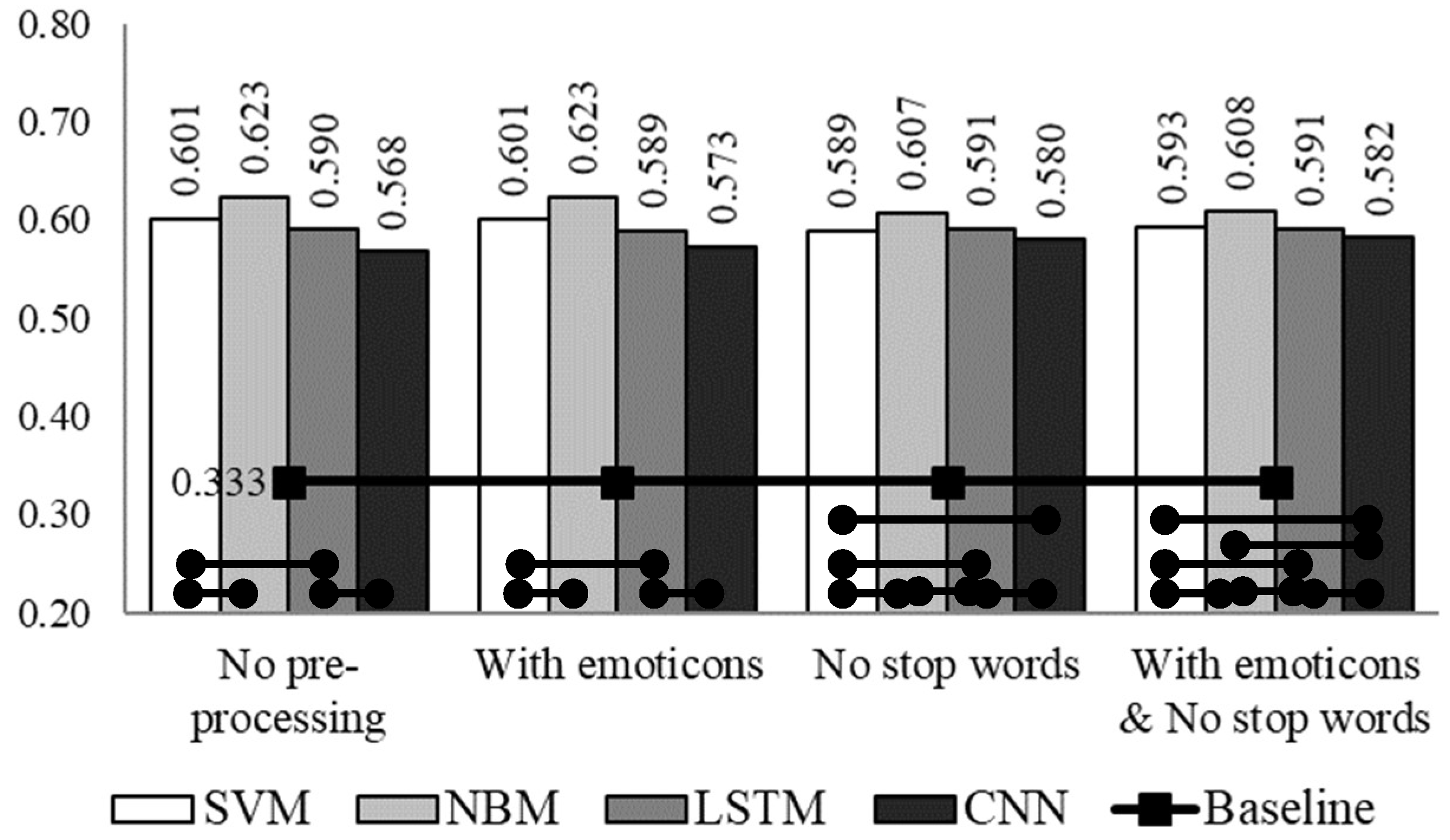
Thus, on the full dataset (in Table 1) baselinerandom = 0.454 and baselinemajority = 0.617, and on the balanced dataset (in Table 2) baselinerandom = baselinemajority = 0.333.
To determine whether the differences between the results are statistically significant, we have performed the McNemar’s test [57] with the significance level equal to 95%. It means that the calculated p-value must be below 0.05, so that the differences would be considered as statistically significant.
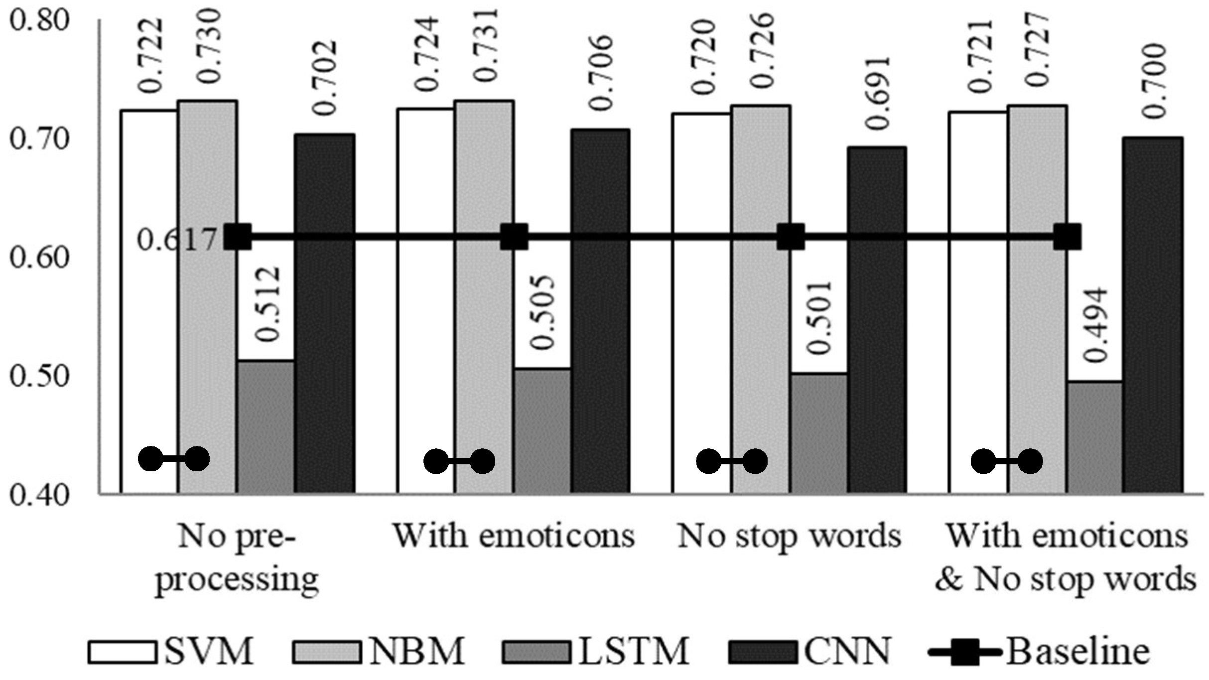
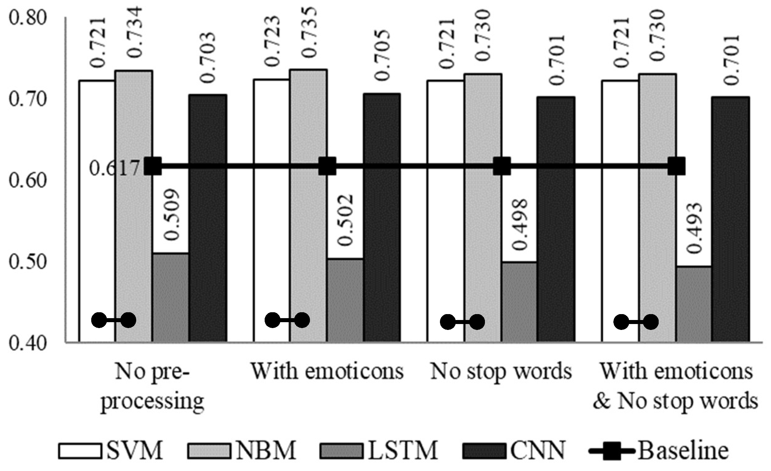
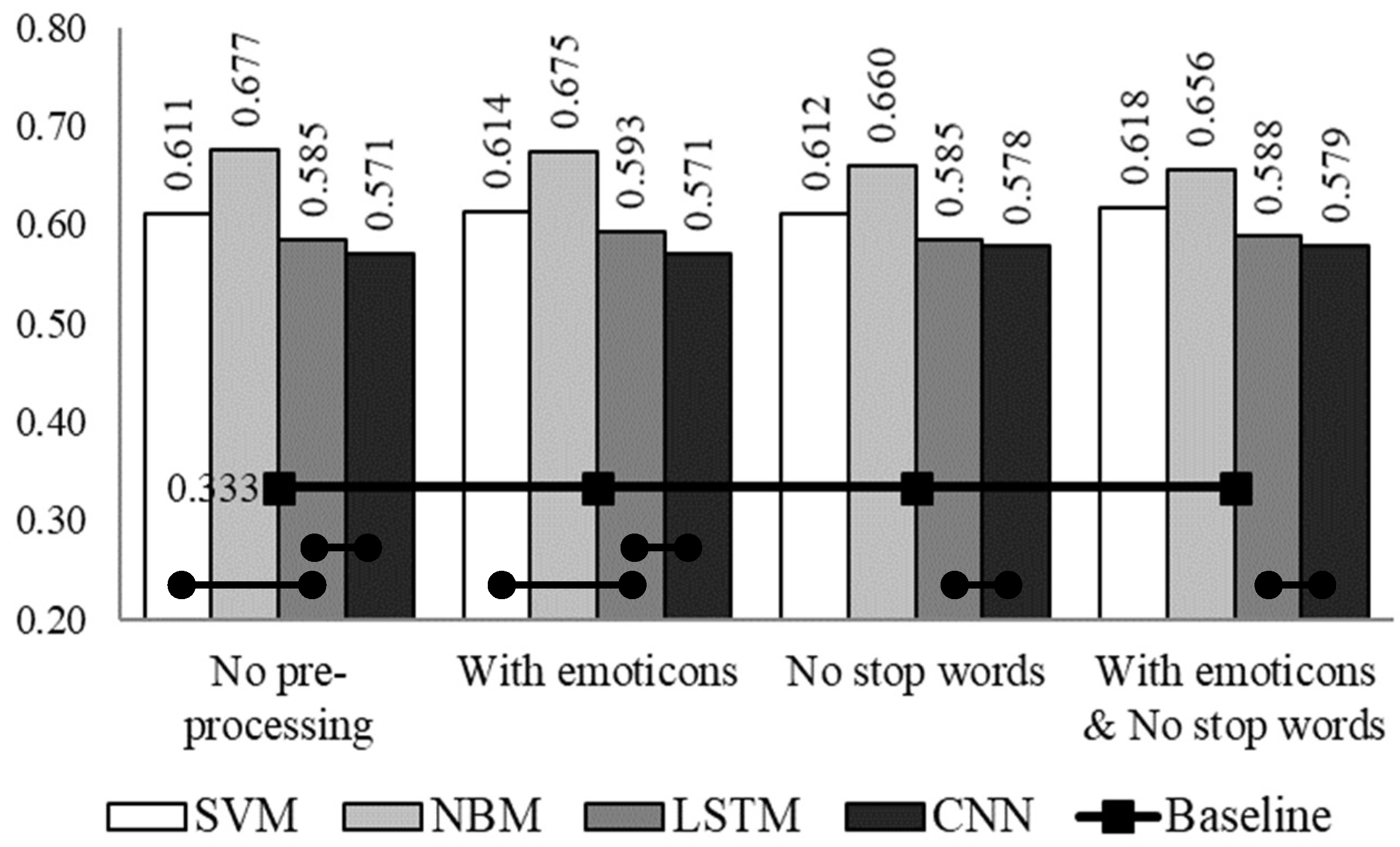
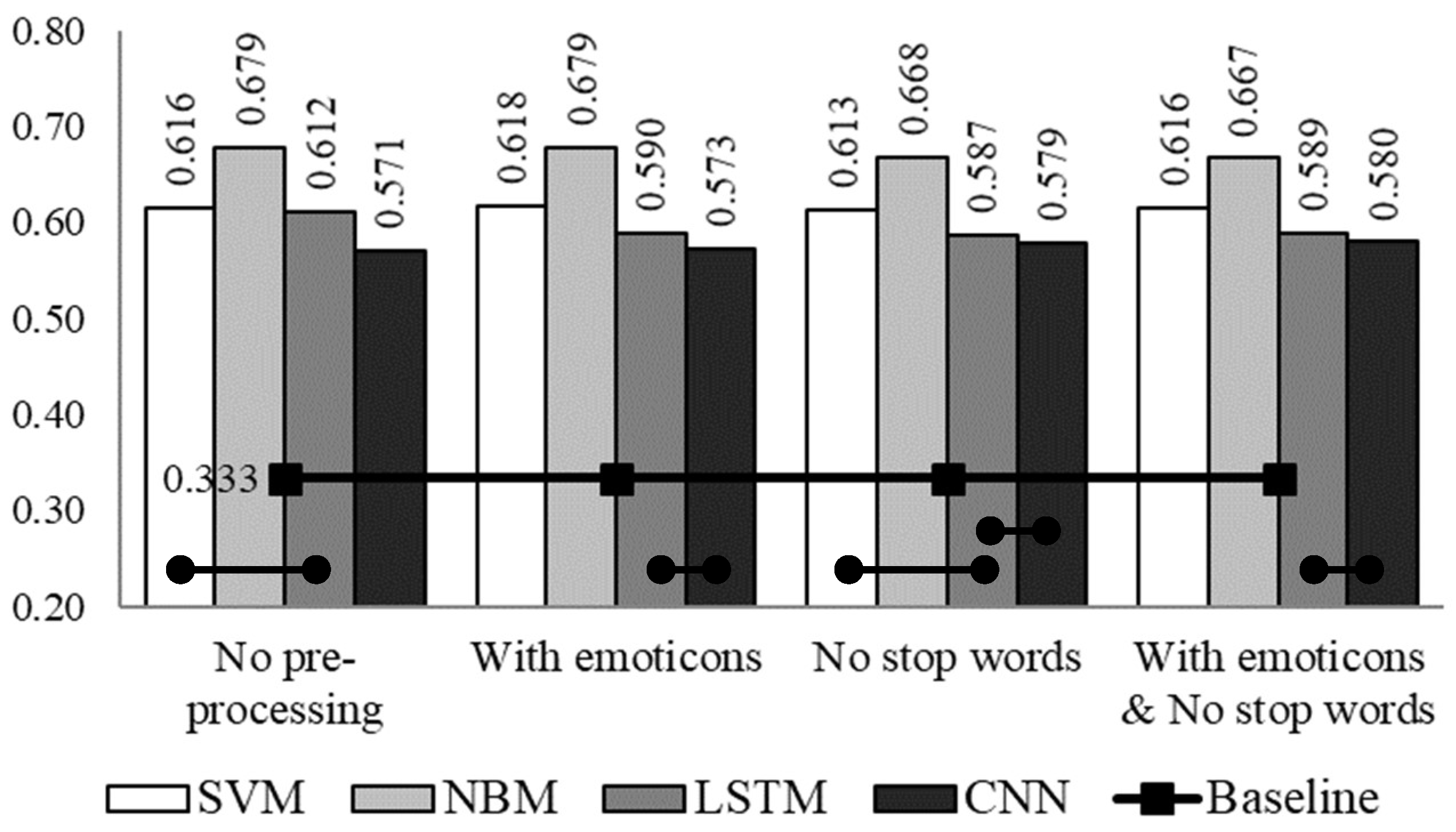
Figure 1, Figure 2 and Figure 3 summarizes the results obtained (1) on the full dataset (presented in Table 1); (2) on the full dataset with eliminated diacritics; and, (3) on the full dataset with restored diacritics, respectively. Figure 4, Figure 5 and Figure 6 present the same pre-processing techniques as in Figure 1, Figure 2 and Figure 3, but applied on the balanced dataset (see Table 2). In Figure 1 and Figure 4, we investigate an accuracy (y axis) of different methods and pre-processing techniques (x axis) on the full and balanced datasets, respectively. It was important to evaluate how accurate methods are on the texts where diacritics are not specifically processed. In Figure 2 and Figure 5, we investigate an impact of diacritics removal: diacritics removal decreases a number of distinct words in the texts, which might positively affect the results but increase the ambiguity (both in the texts and word embeddings), which might have a negative impact on the accuracy. In Figure 3 and Figure 6 we investigate the impact of diacritics restoration. The diacritics restoration should decrease a number of distinct words and reduce the ambiguity; however, here we use the tool that is not refined, therefore some unrecognized words still remain untouched (and undiacritized) in the text.
In the figures for SVM and NBM, we present the highest obtained accuracy values among all feature types: token unigrams (lex1), token unigrams + bigrams (lex2), lemma unigrams (lem1), lemma unigrams + bigrams (lem2), and character tetra-grams (chr4). For LSTM and CNN, we present the highest accuracy values among these types of embeddings: continuous bag-of-words of 300 dimensions with the negative sampling (Word2Vec) and the FastText. Besides, on the texts with the eliminated diacritics, we test the third type, i.e., distorted Word2Vec (marked as Word2Vec_d) (explained in Section 2.4). The best determined feature and embedding types are presented in Table 3 and Table 4 on the full and balanced datasets, respectively.
Some of the SVM and NBM values presented in Figure 4 and Figure 5 were obtained during previous research (presented in [35]). Previously obtained values, together with the new values (obtained with bigrams + unigrams of lemmas during this research), were used for comparison purposes: the best determined feature types and their values (of the same method) are presented in Figure 4 and Figure 5. Only two of 24 values for LSTM and CNN that were presented in Figure 4, Figure 5 and Figure 6 were reused from the previous research (described in [58]). Both old and new values were used for the comparison purposes to choose the best ones. However, the FastText embeddings (used in this research) in most of the cases outperformed Word2Vec (used in the previous research). All other presented values were obtained only during this research.

4. Discussion

Some useful resources as, e.g., SentiWordNet, are not available for the Lithuanian language and it prevents us from solving the sentiment analysis task with effective dictionary-based methods. Besides, lexical resources can usually be used with the normative texts not containing foreign language insertions, jargon, abbreviations, or words with missing diacritics. Not having effective solutions to restore diacritics in the Lithuanian texts (grazusgražus (beautiful)), these lexical recourses cannot be useful. Moreover, even if diacritics could be restored correctly, the currently available Lithuanian morphological tools are not able to recognize non-normative words (e.g., fainą (Anglicism of word fine in accusative)) and transform them into lemma (fainąfainas). Since the dictionary-based methods cannot be effectively applied on the Lithuanian language, machine learning approaches seem as the only possible solution. Of course, due to same previously mentioned reasons about the Lithuanian language specifics (in Section 2.2), we cannot expect the accuracy for the Lithuanian language above 80% (as it is reported in most sentiment analysis research works for the English language). For instance, the sentiment classification on the morphologically complex Croatian language with SVM method reaches ~57% of the f-score on the general topic and ~72% on the specific domain [59]. The authors in [60] solved the sentiment analysis task for Czech on the Facebook posts with Maximum Entropy and SVM and the best achieved f-score is 69%. The deep learning approaches are still not very popular for the morphologically complex languages in the sentiment analysis task. However, the authors in [61] successfully applied the neural network classifier on the Russian language and achieved better results (i.e., 72%) over Logistic Regression, SVM, and Gradient Boosting.
The accuracy strongly depends on the choice of the method. Traditional supervised machine learning approaches seem to be the best solution when training datasets are rather small and more sophisticated feature types (based not only on the lexical, but on the character information) can be tested. Even knowing that the deep learning might not be the best solution for our solving task (because large training datasets and the comprehensive list of word embeddings are not available), we still have to find out how far we may go in the current situation (with the available resources) to know how much efforts on the improvement do we need in the future.
Our results that are represented in Figure 1, Figure 2, Figure 3, Figure 4, Figure 5 and Figure 6 exceed random and majority baselines, except for the LSTM method on the full dataset. It is surprising, because on the balanced dataset LSTM not only exceeds the baseline, but it is superior to CNN. However, LSTM by its nature is well adjusted to deal with the long sequence inputs, which is not that important in our case. We do not need the method to learn what goes in the sequence, we need the method to learn how to classify the text as the whole based on the discriminative n-grams (words/short phrases) that may appear anywhere in the text. Since LSTM yielded the worst performance, we do not analyze it further in more detail.
As we can see from Figure 1, Figure 2, Figure 3, Figure 4 and Figure 5, the accuracy values on the balanced dataset versions are lower as compared to the appropriate full dataset. Despite that the unbalanced datasets may be biased towards the major classes, it is not in our case, because we are dealing with the small data: balancing discards some potentially important information, which is crucial for training the robust model.
Despite that the deep learning techniques underperform traditional machine learning on both datasets a boost from the balanced to full dataset versions is the largest for the CNN method: i.e., 0.116, 0.124, and 0.127 on the original dataset, the dataset with eliminated diacritics, and the dataset with restored diacritics, respectively. For instance, a boost for NBM on the same versions of the dataset is only 0.060, 0.055, and 0.117, respectively; for SVM, it is 0.101, 0.106, and 0.126, respectively. The results confirm the well-known fact [21] that deep learning methods require larger training sets to outperform or to achieve the same accuracy levels as the traditional machine learning approaches. Unfortunately, in our research, even the full dataset is not enough for CNN to outperform SVM or NBM, and these findings coincide with work the presented in [28]. However, using larger datasets is not a straightforward task due to the lack of annotated language resources.
The best overall accuracy with NBM, SVM, and CNN is 0.735, 0.724, and 0.706, respectively. The best performance with NBM was achieved with replaced emoticons, restored diacritics, and lemma unigrams as the feature type. SVM demonstrated the highest accuracy with the replaced emoticons, eliminated diacritics, and lemma unigrams. In case of CNN, the best results were achieved with the replaced emoticons, eliminated diacritics, and the TastText word embeddings. The difference between the best achieved accuracies of NBM and SVM is not statistically significant with p = 0.128, but the differences in accuracies between SVM and CNN, or NBM and CNN are significant with p = 0.014, and very significant with p = 0.000.
The differences between many values are statistically insignificant (especially on the dataset of restored diacritics in Figure 6) on the balanced dataset and it stops us from drawing the conclusions. However, the full dataset of differences among the traditional machine learning methods are also insignificant, but are significant in case of CNN (see p-values obtained with the McNemar test on the full dataset in Table 5).
Although only marginally, different pre-processing techniques also affect the accuracy. From the results we can make the following statements. Restoration of emoticons (positively affecting the accuracy) really helps to express the sentiments; whereas, stop words seems to carry important information, therefore either the removal of stop words should not be applied as the pre-processing technique or the list of stop words has to be carefully examined. Despite their small impact, both elimination and restoration of diacritics and the pre-processing techniques positively affect the results (e.g., without pre-processing CNN achieves 0.691 of accuracy on the full dataset, 0.702 on the dataset with eliminated diacritics, and 0.703 with restored diacritics). Although, in this example, the restoration of diacritics seems to be the better choice when compared to elimination, it is not always the case: e.g., the results for the SVM without pre-processing are lower on the full dataset with restored diacritics (0.721) than on the full dataset with eliminated diacritics (0.722). Despite that it is hard to select the winner (between diacritics elimination and restoration), the diacritics pre-processing in general should be taken into account, especially when dealing with non-normative Lithuanian texts. The accuracy of diacritics restoration depends on the quality of the diacritics restoration tool as well. The tool is not 100% accurate, and sometimes even small errors can lead to the absolutely different meanings and sentiments. Besides, the elimination of diacritics was also used in the Word2Vec embeddings, unfortunately, not very successfully. This failure was probably caused by the loss of some important information: sometimes even slight differences, e.g., gera (good in feminine, singular, nominative) and gerą (good in feminine, singular, accusative), may cause the mapping of words to the absolutely different embeddings. We assume it was the main reason why distorted Word2Vec_d embeddings were outperformed with FastText, which often includes both forms (undiacritized and diacritized) of word embeddings.
The FastText embeddings are effective not only on the texts with eliminated diacritics. The FastText embeddings that are applied on the top of the CNN method are the most effective (see Table 3 and Table 4) word embedding type in general on both dataset versions with all pre-processing techniques and there are two explanations for that. First, the FastText embeddings map more words (two-million word embeddings) as compared to Word2Vec (containing only ~688 thousand of words). Second, Word2Vec embeddings are trained on the normative texts (that do not contain jargon, borrowings, abbreviations, foreign language insertions that also express sentiments) and we assume that FastText embeddings are already trained on the non-normative texts that according to their character are much closer to the texts that we are dealing with in this research.
If the type of word embeddings (i.e., FastText) is obvious when used with CNN, there is still no clear answer as to which feature type is the best for the traditional machine learning techniques. Surprisingly, the character n-grams (usually demonstrating high performance on the non-normative texts) and more sophisticated feature types based on unigrams + bigrams (except for NBM on the balanced original dataset and the dataset with eliminated diacritics) are not the best choice. It is probably due to the fact that the sentiments that we are dealing with are expressed rather straightforward (i.e., without hidden meanings or sarcasm). The top notch feature types for traditional machine learning approaches are token unigrams and lemma unigrams, besides, lemma unigrams are even more often determined to be the best (see Table 3 and Table 4). The credit also goes to the morphological analyzer-lemmatizer tool Lemuoklis: although, it cannot process non-normative words (leaving them in the original form), but it is very accurate when lemmatizing the words that it recognizes.

5. Conclusions

Our main contribution is the comparative analysis of the traditional machine learning and deep learning methods solving the sentiment analysis task for the Lithuanian language. During this work, we have compared Support Vector Machine and Naïve Bayes Multinomial as representatives of traditional machine learning and Long Short-Term Memory and Convolutional Neural Network as representatives of deep learning. The traditional machine learning methods were used with the discrete representations (lexical, lemma, and character feature types); and, the deep learning methods were applied on the top of two types of neural word embeddings (continuous bag-of-words with the negative sampling and the FastText). Moreover, all of the experiments were carried out on the full and the balanced versions of the dataset testing the following pre-processing techniques: emoticons replacement with the sentiment words, stop words removal, diacritics elimination, and restoration.
The LSTM method underperformed the baseline (equal to 0.617 of accuracy) on the full dataset with all of the pre-processing techniques. Another deep learning method, i.e., Convolutional Neural Network, which reached the highest accuracy of 0.706 with FastText embeddings on the full dataset, replaced emoticons, and eliminated diacritics—remained in the third position (our results are very similar when compared to the results achieved with the neural network on the Russian language in [61]). The Support Vector Machine took the second place with the accuracy of 0.724, which was achieved on the full dataset with replaced emoticons, eliminated diacritics, and lemma unigrams as the feature representation type. The best result was demonstrated by the Naïve Bayes Multinomial method with the accuracy of 0.735, which was achieved on the full dataset, replaced emotions, restored diacritics, and lemma unigrams. Although Convolutional Neural Network underperformed Support Vector Machine and Naïve Bayes Multinomial, the gap in the accuracy is rather small, i.e., less than 0.3.
In the further research, we plan to reduce (or even eliminate) the gap between traditional and deep learning approaches. This could be done in two directions: (1) by modifying the parameters of the deep learning approaches; and, (2) by collecting and preparing more training data. Moreover, we envision the development of hybrid methods, such as advocated in [62], which combine neural networks with explicit knowledge.

Author Contributions

Formal analysis, M.W.; Software, J.K.-D.; Visualization, J.K.-D.; Writing—original draft, J.K.-D.; Writing—review and editing, R.D.

Funding

This research received no external funding.

Conflicts of Interest

The authors declare that there is no conflict of interests regarding publication of this paper.

References

  1. Htet, H.; Khaing, S.S.; Myint, Y.Y. Tweets sentiment analysis for healthcare on big data processing and IoT architecture using maximum entropy classifier. In Proceedings of the International Conference on Big Data Analysis and Deep Learning Applications, Miyazaki, Japan, 14–15 May 2018; Zin, T., Lin, J.W., Eds.; Springer: Singapore, 2019; Volume 744, pp. 28–38. [Google Scholar] [CrossRef]
  2. Moe, Z.H.; San, T.; Tin, H.M.; Hlaing, N.Y.; Tin, M.M. Evaluation for teacher’s ability and forecasting student’s career based on big data. In Big Data Analysis and Deep Learning Applications; Springer: Singapore, 2019. [Google Scholar] [CrossRef]
  3. Agarwal, B.; Mittal, N.; Bansal, P.; Garg, S. Sentiment Analysis Using Common-Sense and Context Information. Comput. Intell. Neurosci. 2015, 2015. [Google Scholar] [CrossRef] [PubMed]
  4. Asghar, M.Z.; Khan, A.; Ahmad, Sh.; Qasim, M.; Khan, I.A. Lexicon-enhanced sentiment analysis framework using rule-based classification scheme. PLoS ONE 2017, 12, e0171649. [Google Scholar] [CrossRef] [PubMed]
  5. Augustyniak, Ł.; Szymański, P.; Kajdanowicz, T.; Tuligłowicz, W. Comprehensive study on lexicon-based ensemble classification sentiment analysis. Entropy 2016, 18, 4. [Google Scholar] [CrossRef]
  6. Dilawar, N.; Majeed, H.; Beg, M.O.; Ejaz, N.; Muhammad, K.; Mehmood, I.; Nam, Y. Understanding citizen issues through reviews: A step towards data informed planning in smart cities. Appl. Sci. 2018, 8, 1589. [Google Scholar] [CrossRef]
  7. Ravichandran, M.; Kulanthaivel, G.; Chellatamilan, T. Intelligent Topical Sentiment Analysis for the Classification of E-Learners and Their Topics of Interest. Sci. World J. 2015, 2015, 617358. [Google Scholar] [CrossRef] [PubMed]
  8. Ferrara, E.; Yang, Z. Quantifying the Effect of Sentiment on Information Diffusion in Social Media. PeerJ Comput. Sci. 2015, 1, e26. [Google Scholar] [CrossRef]
  9. Martinčić-Ipšić, S.; Močibob, E.; Perc, M. Link prediction on Twitter. PLoS ONE 2017, 12, e0181079. [Google Scholar] [CrossRef] [PubMed]
  10. Wang, X.; Zhang, H.; Yuan, S.; Wang, J.; Zhou, Y. Sentiment processing of social media information from both wireless and wired network. Eur. J. Wirel. Commun. Netw. 2016, 164. [Google Scholar] [CrossRef]
  11. Ranco, G.; Bordino, I.; Bormetti, G.; Caldarelli, G.; Lillo, F.; Treccani, M. Coupling News Sentiment with Web Browsing Data Improves Prediction of Intra-Day Price Dynamics. PLoS ONE 2016, 11, e0146576. [Google Scholar] [CrossRef] [PubMed]
  12. Taboada, M.; Brooke, J.; Tofiloski, M.; Voll, K.; Stede, M. Lexicon-Based Methods for Sentiment Analysis. Comput. Linguist. 2011, 37, 267–307. [Google Scholar] [CrossRef]
  13. Turney, P.D. Thumbs Up or Thumbs Down? Semantic Orientation Applied to Unsupervised Classification of Reviews. In Proceedings of the 40th Annual Meeting on Association for Computational Linguistics, 2002, ACL’02, Philadelphia, PA, USA, 7–12 July 2002; pp. 417–424. [Google Scholar] [CrossRef]
  14. De Diego, I.M.; Fernández-Isabel, A.; Ortega, F.; Moguerza, J.M. A visual framework for dynamic emotional web analysis. Knowl. Based Syst. 2018, 145, 264–273. [Google Scholar] [CrossRef]
  15. Socher, R.; Perelygin, A.; Wu, J.; Chuang, J.; Manning, C.D.; Ng, A.; Potts, C. Recursive deep models for semantic compositionality over a sentiment treebank. In Proceedings of the 2013 Conference on Empirical Methods in Natural Language Processing, Seattle, Washington, DC, USA, 18–21 October 2013; pp. 1631–1642. [Google Scholar]
  16. Pak, A.; Paroubek, P. Twitter for Sentiment Analysis: When Language Resources are Not Available. In Proceedings of the Database and Expert Systems Applications (DEXA 2011), Toulouse, France, 29 August–2 September 2011; pp. 111–115. [Google Scholar] [CrossRef]
  17. Pang, B.; Lee, L.; Vaithyanathan, S. Thumbs up? Sentiment Classification using Machine Learning Techniques. In Proceedings of the Conference on Empirical Methods in Natural Language Processing, EMNLP, Honolulu, HI, USA, 25–27 October 2002; pp. 79–86. [Google Scholar] [CrossRef]
  18. Nogueira dos Santos, C.; Maira, G. Deep Convolutional Neural Networks for Sentiment Analysis of Short Texts. In Proceedings of the 25th International Conference on Computational Linguistics (COLING), Dublin, Ireland, 23–29 August 2014; pp. 69–78. [Google Scholar]
  19. Pang, B.; Lee, L. Seeing stars: Exploiting class relationships for sentiment categorization with respect to rating scales. In Proceedings of the Association for Computational Linguistics (ACL), Ann Arbor, MI, USA, 25–30 June 2005; pp. 115–124. [Google Scholar] [CrossRef]
  20. Go, A.; Bhayani, R.; Huang, L. Twitter Sentiment Classification using Distant Supervision. Available online: https://cs.stanford.edu/people/alecmgo/papers/TwitterDistantSupervision09.pdf (accessed on 30 December 2018).
  21. Katoh, K.; Ninomiya, T. Deep Learning for Large-Scale Sentiment Analysis Using Distributed Representations. In Proceedings of the SEMAPRO 2015: The 9th International Conference on Advances in Semantic Processing, Nice, France, 19–24 July 2015; pp. 92–96. [Google Scholar]
  22. Severyn, A.; Moschitti, A. Twitter Sentiment Analysis with Deep Convolutional Neural Networks. In Proceedings of the 38th International ACM SIGIR Conference on Research and Development in Information Retrieval, SIGIR’15, Santiago, Chile, 9–13 August 2015; pp. 959–962. [Google Scholar] [CrossRef]
  23. Guan, Z.; Chen, L.; Zhao, W.; Zheng, Y.; Tan, S.; Cai, D. Weakly-Supervised Deep Learning for Customer Review Sentiment Classification. In Proceedings of the International Joint Conference on Artificial Intelligence, New York, NY, USA, 9–15 July 2016; pp. 3719–3725. [Google Scholar]
  24. Akhtar, M.S.; Kumar, A.; Ekbal, A.; Bhattacharyya, P. A Hybrid Deep Learning Architecture for Sentiment Analysis. In Proceedings of the COLING 2016, the 26th International Conference on Computational Linguistics: Technical Papers, Osaka, Japan, 11–16 December 2016; pp. 482–493. [Google Scholar]
  25. Yousif, A.; Niu, Z.; Nyamawe, A.S.; Hu, Y. Improving citation sentiment and purpose classification using hybrid deep neural network model. In Proceedings of the International Conference on Advanced Intelligent Systems and Informatics, AISI 2018, Cairo, Egypt, 1–3 September 2018; pp. 327–336. [Google Scholar] [CrossRef]
  26. Yun, W.; An, W.X.; Jindan, Z.; Yu, C. Combining vector space features and convolution neural network for text sentiment analysis. In Proceedings of the CISIS 2018: Complex, Intelligent, and Software Intensive Systems, Osaka, Japan, 4–6 July 2018; pp. 780–790. [Google Scholar] [CrossRef]
  27. Stojanovski, D.; Strezoski, G.; Madjarov, G.; Dimitrovski, I. Finki at SemEval-2016 Task 4: Deep Learning Architecture for Twitter Sentiment Analysis. In Proceedings of the 10th International Workshop on Semantic Evaluation (SemEval-2016), San Diego, CA, USA, 16–17 June 2016; pp. 149–154. [Google Scholar]
  28. Lu, Y.; Sakamoto, K.; Shibuki, H.; Mori, T. Are Deep Learning Methods Better for Twitter Sentiment Analysis? Available online: http://www.anlp.jp/proceedings/annual_meeting/2017/pdf_dir/C5-1.pdf (accessed on 30 December 2018).
  29. Cortis, K.; Freitas, A.; Daudert, T.; Hürlimann, M.; Zarrouk, M.; Handschuh, S.; Davis, B. SemEval-2017 Task 5: Fine-Grained Sentiment Analysis on Financial Microblogs and News. In Proceedings of the 11th International Workshop on Semantic Evaluation, SemEval-2017, Vancouver, BC, Canada, 3–4 August 2017; pp. 519–535. [Google Scholar]
  30. Jiang, M.; Lan, M.; Wu, Y. ECNU at SemEval-2017 Task 5: An Ensemble of Regression Algorithms with Effective Features for Fine-Grained Sentiment Analysis in Financial Domain. In Proceedings of the 11th International Workshop on Semantic Evaluation, SemEval-2017, Vancouver, BC, Canada, 3–4 August 2017; pp. 888–893. [Google Scholar]
  31. Ghosal, D.; Bhatnagar, S.; Akhtar, M.S.; Ekbal, A.; Bhattacharyya, P. IITP at SemEval-2017 Task 5: An Ensemble of Deep Learning and Feature Based Models for Financial Sentiment Analysis. In Proceedings of the 11th International Workshop on Semantic Evaluation, SemEval-2017, Vancouver, BC, Canada, 3–4 August 2017; pp. 899–903. [Google Scholar]
  32. Rosenthal, S.; Farra, N.; Nakov, P. SemEval-2017 Task 4: Sentiment Analysis in Twitter. In Proceedings of the 11th International Workshop on Semantic Evaluation, SemEval-2017, Vancouver, BC, Canada, 3–4 August 2017; pp. 502–518. [Google Scholar]
  33. Cliché, M. BB_twtr at SemEval-2017 Task 4: Twitter Sentiment Analysis with CNNs and LSTMs. In Proceedings of the 11th International Workshop on Semantic Evaluation, SemEval-2017, Vancouver, BC, Canada, 3–4 August 2017; pp. 573–580. [Google Scholar]
  34. Baziotis, C.; Pelekis, N.; Doulkeridis, C. DataStories at SemEval-2017 Task 4: Deep LSTM with Attention for Message-level and Topic-based Sentiment Analysis. In Proceedings of the 11th International Workshop on Semantic Evaluation, SemEval-2017, Vancouver, BC, Canada, 3–4 August 2017; pp. 747–754. [Google Scholar]
  35. Kapočiūtė-Dzikienė, J.; Krupavičius, A.; Krilavičius, T. A Comparison of Approaches for Sentiment Classification on Lithuanian Internet Comments. In Proceedings of the 4th Biennial International Workshop on Balto-Slavic Natural Language Processing, Sofia, Bulgaria, 8–9 August 2013; pp. 2–11. [Google Scholar]
  36. Naktinienė, G.; Paulauskas, J.; Petrokienė, R.; Vitkauskas, V.; Zabarskaitė, J. (Eds.) Lietuvių Kalbos Žodynas (t. 1-20, 1941–2002): Elektroninis Variantas [Lithuanian Language Dictionary (Vol. 1-20, 1941–2002): Electronic version]; Lietuvių Kalbos Institutas: Vilnius, Lithuania, 2005. (In Lithuanian) [Google Scholar]
  37. Stevenson, A. (Ed.) Oxford Dictionary of English, 3th ed.; Oxford University Press: Oxford, UK, 2010. [Google Scholar]
  38. Urbutis, U. Žodžių Darybos Teorija [Word Derivation Theory]; Mokslo ir Enciklopedijų Leidybos Institutas: Vilnius, Lithuania, 2009. (In Lithuanian) [Google Scholar]
  39. Read, J. Using Emoticons to Reduce Dependency in Machine Learning Techniques for Sentiment Classification. In Proceedings of the ACL Student Research Workshop, ACL’05, Ann Arbor, MI, USA, 27 June 2005; pp. 43–48. [Google Scholar]
  40. Spencer, J.; Uchyigit, G. Sentimentor: Sentiment Analysis on Twitter Data. In Proceedings of the 1st International Workshop on Sentiment Discovery from Affective Data, Bristol, UK, 28 September 2012; pp. 56–66. [Google Scholar]
  41. Kapočiūtė-Dzikienė, J.; Davidsonas, A.; Vidugirienė, A. Character-Based Machine Learning vs. Language Modeling for Diacritics Restoration. Inf. Technol. Control 2017, 46, 508–520. [Google Scholar] [CrossRef]
  42. Cortes, C.; Vapnik, V. Support vector networks. Mach. Learn. 1997, 20, 273–297. [Google Scholar] [CrossRef]
  43. Joachims, T. Text Categorization with Support Vector Machines: Learning with many Relevant Features. In Proceedings of the 10th European Conference on Machine Learning, ECML-98, Chemnitz, Germany, 21–23 April 1998; Volume 1398, pp. 137–142. [Google Scholar] [CrossRef]
  44. Lewis, D.D.; Gale, W.A. A sequential algorithm for training text classifiers. In Proceedings of the 17th Annual International ACM-SIGIR Conference on Research and Development in Information Retrieval, SIGIR-94, Dublin, Ireland, 3–6 July 1994; pp. 3–12. [Google Scholar]
  45. Zinkevičius, V. Lemuoklis—Morfologinei analizei [Morphological analysis with Lemuoklis]. In Darbai ir Dienos; Gudaitis, L., Ed.; VDU Leidykla: Kaunas, Lithuania, 2000; Volume 24, pp. 246–273. (In Lithuanian) [Google Scholar]
  46. Kapočiūtė-Dzikienė, J.; Vaassen, F.; Daelemans, W.; Krupavičius, A. Improving topic classification for highly inflective languages. In Proceedings of the 24th International Conference on Computational Linguistics (COLING 2012), Mumbai, India, 8–15 December 2012; pp. 1393–1410. [Google Scholar]
  47. Hochreiter, S.; Schmidhuber, J. Long Short-Term Memory. Neural Comput. 1997, 9, 1735–1780. [Google Scholar] [CrossRef] [PubMed]
  48. Lecun, Y.; Bottou, L.; Bengio, Y.; Haffner, P. Gradient-based learning applied to document recognition. Proc. IEEE 1998, 2278–2324. [Google Scholar] [CrossRef]
  49. Kim, Y. Convolutional Neural Networks for Sentence Classification. In Proceedings of the Empirical Methods in Natural Language Processing, EMNLP, Doha, Qatar, 25–29 October 2014; pp. 1746–1751. [Google Scholar] [CrossRef]
  50. Graves, A. Supervised Sequence Labelling with Recurrent Neural Networks; Springer: Berlin/Heidelberg, Germany, 2012; pp. 11–31. ISBN 978-3-642-24796-5. [Google Scholar]
  51. Open-Source, Distributed, Deep Learning Library for the JVM. Available online: https://deeplearning4j.org/ (accessed on 30 December 2018).
  52. Mikolov, T.; Chen, K.; Corrado, G.; Dean, J. Efficient Estimation of Word Representations in Vector Space. arXiv, 2013; arXiv:1301.3781. [Google Scholar]
  53. Mikolov, T.; Sutskever, I.; Chen, K.; Corrado, G.S.; Dean, J. Distributed Representations of Words and Phrases and their Compositionality. In Proceedings of the 27th Annual Conference on Neural Information Processing Systems, Lake Tahoe, NV, USA, 5–10 December 2013; pp. 3111–3119. [Google Scholar]
  54. Kapočiūtė-Dzikienė, J.; Damaševičius, R. Intrinsic evaluation of Lithuanian word embeddings using WordNet. In Proceedings of the CSOC 2018: 7th Computer Science On-Line Conference, Zlin, Czech Republic, 25–28 April 2018; pp. 394–404. [Google Scholar] [CrossRef]
  55. Grave, E.; Bojanowski, P.; Gupta, P.; Joulin, A.; Mikolov, T. Learning Word Vectors for 157 Languages. In Proceedings of the International Conference on Language Resources and Evaluation (LREC 2018), Miyazaki, Japan, 7–12 May 2018. [Google Scholar]
  56. Sokolova, M.; Lapalme, G. A Systematic Analysis of Performance Measures for Classification Tasks. Inf. Process. Manag. 2009, 45, 427–437. [Google Scholar] [CrossRef]
  57. McNemar, Q. Note on the sampling error of the difference between correlated proportions or percentages. Psychometrika 1947, 12, 153–157. [Google Scholar] [CrossRef] [PubMed]
  58. Kapočiūtė-Dzikienė, J.; Damaševičius, R.; Wozniak, M. Sentiment analysis of Lithuanian texts using deep learning methods. In Proceedings of the 24th international conference on Information and Software Technologies, (ICIST 2018), Vilnius, Lithuania, 4–6 October 2018; pp. 521–532. [Google Scholar] [CrossRef]
  59. Rotim, L.; Snajder, J. Comparison of Short-Text Sentiment Analysis Methods for Croatian. In Proceedings of the 6th Workshop on Balto-Slavic Natural Language Processing, Valencia, Spain, 4 April 2017; pp. 69–75. [Google Scholar]
  60. Habernal, I.; Ptácek, T.; Steinberger, J. Sentiment Analysis in Czech Social Media Using Supervised Machine Learning. In Proceedings of the 4th Workshop on Computational Approaches to Subjectivity, Sentiment and Social Media Analysis, Atlanta, GA, USA, 14 June 2013; pp. 65–74. [Google Scholar]
  61. Rogers, A.; Romanov, A.; Rumshisky, A.; Volkova, S.; Gronas, M.; Gribov, A. RuSentiment: An Enriched Sentiment Analysis Dataset for Social Media in Russian. In Proceedings of the 27th International Conference on Computational Linguistics (COLING 2018), Santa Fe, NM, USA, 20–26 August 2018; pp. 755–763. [Google Scholar]
  62. Ma, Y.; Peng, H.; Khan, T.; Cambria, E.; Hussain, A. Sentic LSTM: A Hybrid Network for Targeted Aspect-Based Sentiment Analysis. Cogn. Comput. 2018, 10, 639–650. [Google Scholar] [CrossRef]
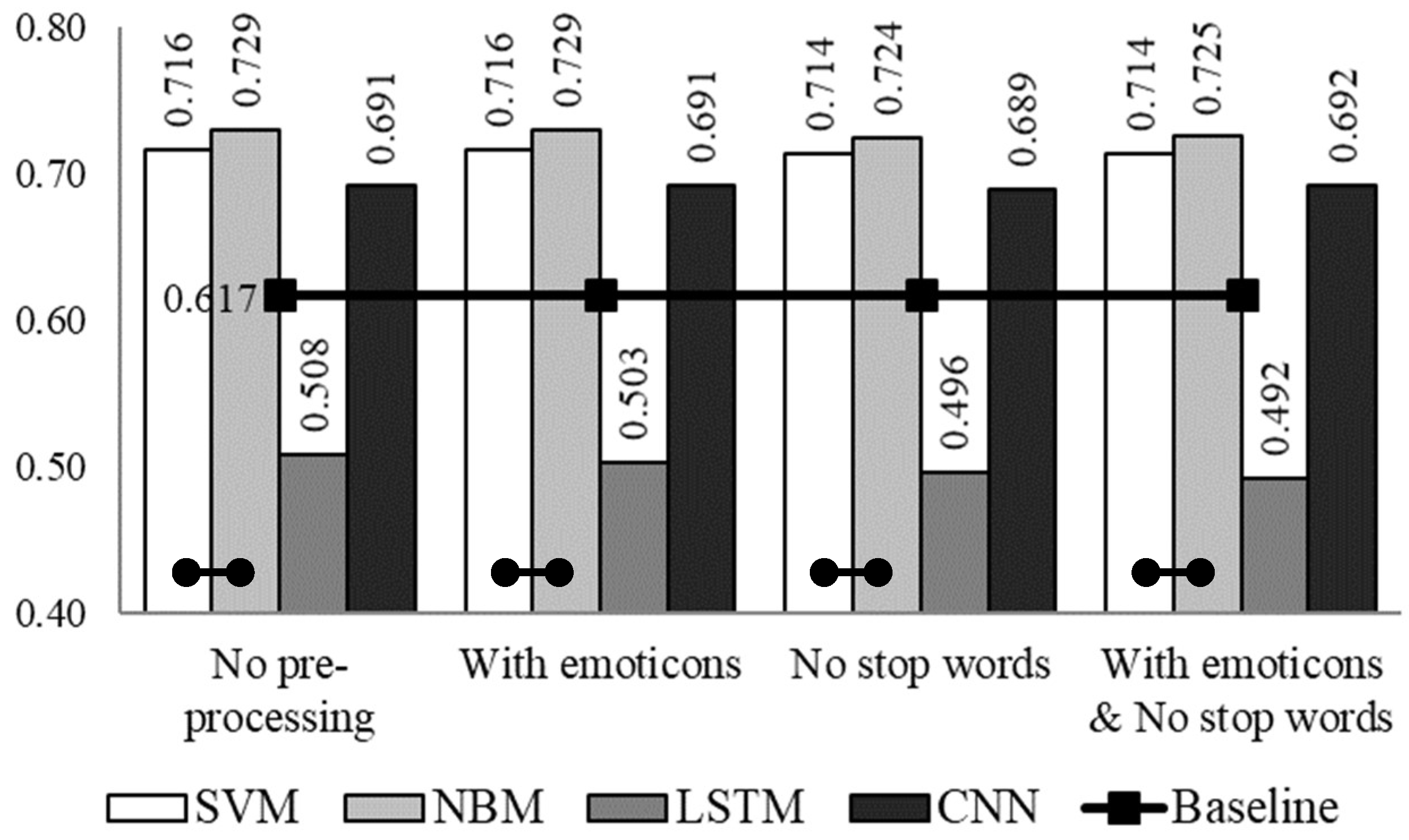
Figure 1. Accuracy obtained with different pre-processing techniques applied on the full dataset. Black connecting lines in each group of columns connect results among which differences are not statistically significant.
Computers 08 00004 g001
Figure 2. Accuracies with different pre-processing on the full dataset with eliminated diacritics.
Computers 08 00004 g002
Figure 3. Accuracies with different pre-processing on the full dataset with restored diacritics.
Computers 08 00004 g003
Figure 4. Accuracies with different pre-processing on the balanced dataset.
Computers 08 00004 g004
Figure 5. Accuracies with different pre-processing on the balanced dataset with eliminated diacritics.
Computers 08 00004 g005
Figure 6. Accuracies with different pre-processing on the balanced dataset with restored diacritics.
Computers 08 00004 g006
Table 1. Statistical characteristics of the full dataset used in our sentiment analysis tasks. The upper and lower value in columns (4)–(6) represent the number of all tokens and the number of distinct tokens, respectively.
Class LabelNumb. of TextsAvg. Text LengthNumb. of TokensTokens with EmoticonsTokens without Stop Words
positive21767.6216,576
4976
16,818
4977
14,609
4902
negative65219.9464,832
20,365
65,159
20,368
54,162
20,307
neutral18738.9816,824
6551
16,884
6552
13,831
6544
total10,5709.2998,232
25,942
98,861
25,945
82,602
25,491
Table 2. Statistical characteristics of the balanced dataset used in our sentiment analysis tasks. The upper and lower value in columns (4)–(6) represent the number of all tokens and the number of distinct tokens, respectively.
Class LabelNumb. of TextsAvg. Text LengthNumb. of TokensTokens with EmoticonsTokens without Stop Words
positive15006.9710,455
3177
10,664
4027
8982
3941
negative150010.0015,000
6475
15,107
7811
11,945
7716
neutral15008.7713,165
5134
13,226
6391
10,427
6276
total45008.5838,621
11,669
38,997
14,966
31,354
14,923
Table 3. The best revealed feature and embedding types with different classification methods on the full dataset.
SVMNBMLSTMCNN
Original
No pre-processinglem1lem1Word2VecFastText
With emoticonslem1lem1Word2VecFastText
No stop wordslex1lex1Word2VecFastText
With emoticons & No stop wordslem1lem1Word2VecFastText
Eliminated Diacrtics
No pre-processinglex1lem1Word2Vec_dFastText
With emoticonslem1lem1Word2VecFastText
No stop wordslex1lex1Word2VecFastText
With emoticons & No stop wordslem1lem1Word2VecFastText
Restored diacritics
No pre-processinglex1lem1Word2VecFastText
With emoticonslex1lem1Word2VecFastText
No stop wordslex1lem1Word2VecFastText
With emoticons & No stop wordslex1lem1Word2VecFastText
Table 4. Best features and embedding types with different classification methods on the balanced dataset.
SVMNBMLSTMCNN
Original
No pre-processinglex1lex2FastTextFastText
With emoticonslem1lex2FastTextFastText
No stop wordslex1lex2FastTextFastText
With emoticons & No stop wordslem1lex2FastTextFastText
Eliminated Diacrtics
No pre-processinglex1lex2Word2VecFastText
With emoticonslex1lex2FastTextFastText
No stop wordslex1lex2FastTextFastText
With emoticons & No stop wordslex1lex2FastTextFastText
Restored diacritics
No pre-processinglem1lem1Word2VecFastText
With emoticonslem1lem1FastTextFastText
No stop wordslem1lem1FastTextFastText
With emoticons & No stop wordslem1lem1FastTextFastText
Table 5. p-values, representing the level of significance between the accuracies of Support Vector Machines (SVM), Naïve Bayes Multinomial (NBM), and Convolutional Neural Network (CNN) presented in Figure 1, Figure 2 and Figure 3. Underlined p-values denote statistically insignificant differences.
Pre-Processing TechniqueCompared Methods
CNN & SVMCNN & NBMSVM & NBM
OriginalNo pre-processing
With emoticons
No stop words
With emoticons & No stop words
0.001
0.001
0.001
0.003
0.000
0.000
0.000
0.000
0.069
0.071
0.165
0.135
Eliminated diacriticsNo pre-processing
With emoticons
No stop words
With emoticons & No stop words
0.007
0.018
0.000
0.004
0.000
0.001
0.000
0.000
0.264
0.330
0.418
0.432
Restored diacriticsNo pre-processing
With emoticons
No stop words
With emoticons & No stop words
0.015
0.015
0.007
0.005
0.000
0.000
0.000
0.000
0.089
0.107
0.222
0.217