Abstract
Cellular beams are an attractive option for the steel construction industry due to their versatility in terms of strength, size, and weight. Further benefits are the integration of services thereby reducing ceiling-to-floor depth (thus, building’s height), which has a great economic impact. Moreover, the complex localized and global failures characterizing those members have led several scientists to focus their research on the development of more efficient design guidelines. This paper aims to propose an artificial neural network (ANN)-based formula to precisely compute the critical elastic buckling load of simply supported cellular beams under uniformly distributed vertical loads. The 3645-point dataset used in ANN design was obtained from an extensive parametric finite element analysis performed in ABAQUS. The independent variables adopted as ANN inputs are the following: beam’s length, opening diameter, web-post width, cross-section height, web thickness, flange width, flange thickness, and the distance between the last opening edge and the end support. The proposed model shows a strong potential as an effective design tool. The maximum and average relative errors among the 3645 data points were found to be 3.7% and 0.4%, respectively, whereas the average computing time per data point is smaller than a millisecond for any current personal computer.
1. Introduction
The use of cellular beams (i.e., perforated beams with circular web openings) in the construction sector has significantly increased over the past decade on account of the distinct and discreet advantages they offer. Cellular beams are applicable for long span structures, where integration of services such as ventilation ducts and lightings systems within the beam is attained, but also for short spans, where spatial interference among concentrated mechanical devices and structural elements may require a compromised solution. Cellular beams allow reducing the height of buildings to fit a required number of floors, otherwise fitting more floors in a given height limit, thus having a significant economic impact to the whole structure’s budget. Furthermore, cellular beams offer practical advantages such as the possibility of (i) fixing the ceilings directly to the beams’ lower flanges instead of requiring additional suspension elements, and (ii) allowing future equipment addition or replacement within the existent void holes. In fact, with the wider adoption of Building Information Modeling (BIM), the knowledge of those expansion possibilities is becoming a valuable asset for the building management.
Long span and lightweight structures also benefit from flexible designs with the fewer number of columns and foundations, and thus from the reduced construction time [1]. The increase in beam depth due to the castellation process (i.e., profile cutting manufacturing) also provides greater flexural stiffness having a final section with larger section modulus [2]. However, the presence of web openings significantly influences the structural performance of the beams, which in particular is dependent on the geometry (shape, diameter, and critical opening length), location (shear-moment interaction), and spacing (closely and widely spaced) between perforations. The perforations lead to complex structural behaviors, attributed to the distribution of forces and stresses in the vicinity of the openings. This results in rather complicated and conservative design procedures ([2,3]).
The first analytical model proposed by Uenoya and Redwood [4] provided critical baseline data relating to the behavior of perforated beams by studying the in-plane stress distribution pattern using perforated plates. Later, Lucas and Darwin [5] proposed a design process based on the identification of the maximum bending and shear capacities at the web openings. It was afterwards suggested that the nominal capacities for the combinations of the bending moment and shear at each opening were determined. This method was accepted by the AISC [6] and the ASCE 23-97 [7]. However, the method only provided a reasonable accurate load estimate for beams with small height, whereas for greater heights becomes conservative. The method is also restrictive to a maximum opening height of 0.7 h, since the average errors were found to increase significantly above this range. Also, in 1990, Ward [8] proposed a simplified semi-empirical web-post model using finite element Modeling; however, this model was restrictive as it was based on a limited number of geometric configurations and best results were found with an error of 30%. Following, Chung et al. [9] studied the Vierendeel mechanism and derived moment-shear interaction curves for various types of perforated beams which ultimately led to the development of a generalized moment-shear curve to assess the load carrying capacities of beams with various openings. In 2003, Chung at al. [10] further analyzed this moment-shear interaction curve and concluded that different shapes and sizes of openings can affect a beam differently and that this curve is more relevant for beams with large openings. In the same year, Chung et al. [10] reported that the moment-shear curve can be somewhat conservative when analyzing beams with small web openings. However, Chung et al.’s findings were identified as a relatively good method as it provided a good approximation with mean errors of 15–25% (for various shapes of web openings), where cellular beams indicated an error of 15.8%. Since 2009, Tsavdaridis et al. published studies [1,11,12,13,14] on thin-walled perforated beams with circular and other novel non-standard web openings investigating the web-post buckling failure mode for closely spaced web openings as well as the Vierendeel mechanism when large isolated web openings. The studies revealed that the Vierendeel bending is influenced by both the shape and size of an opening and the load carrying capacity of beams with large web openings can be found by examining the formation (the order and position) of plastic hinges. The extreme opening diameter (0.8 h) as opposed to the maximum value of 0.75 h presented in earlier literature, was introduced by Tsavdaridis and D’Mello [13] in order to comprehensively develop an understanding of the parameters which affect the structural behavior of perforated beams. Akrami and Erfani (2016), in a comparative analysis of the design methodologies for perforated beams, found that the works of Chung et al [10] and Tsavdaridis and D’Mello [13] were less restrictive as compared to other design methods (ASCE 23-97, SCI-P100, SCI-P355) and produce the lowest errors. In 2011, Lawson and Hicks [15] published the SCI-P355 design guidelines, an update to SCI-P068 [16] and SCI-P100 [8] which proposed that the Vierendeel bending resistance is dependent on the classification of the web of the T-beams. This approach produced acceptable approximations for openings of specific dimensions where the best results were found with an error of 25–30%. It is worth noting that Chung et al. [10], Verweij [17] and Morkhade and Gupta [2] have reported that the current guidelines, specifically SCI-P100 [8] and SCI-P355 [15], are inadequate, complicated, and conservative when it comes to the design of perforated steel beams.
Artificial neural networks (ANN) have become a popular method to predict the response of structures. Gholizadeh et al. [18] presented a study relating the use of ANN in the evaluation of the load carrying capacity of the web-post of castellated steam beams based on 140 FE models. The computational technique generated predictions with great accuracy when compared to other methods. Sharifi and Tohidi [19] also illustrated the application of ANN to accurately estimate the elastic buckling load capacity of steel bridge girders that have rectangular openings at the bottom zone in the web. This is considered as the worse possible location to place an opening to resist lateral torsional buckling. The ANN formula was derived from 21 FE models which managed to accurately predict the elastic buckling load. In 2014, Tohidi and Sharifi [20] demonstrated the versatility of ANN by studying the buckling capacity of steel beams with rectangular web openings that has experienced corrosion in the web. In addition, Tohidi and Sharifi [21] developed an ANN model to estimate the bearing capacity of steel girders with corrosion at the bearing region. The ANN empirical formulas obtained were reported to be accurate in predicting the residual capacity of deteriorated steel beams. Examples of recent and relevant works concerning the application of ANN to other types of structures within civil engineering read [22,23,24,25].
The current study was motivated by the lack of rational (simple, efficient, and accurate) design procedures relating to the buckling response of cellular beams. This paper proposes an ANN-based formula to precisely compute the critical elastic buckling load of simply supported cellular beams under uniformly distributed vertical loads, as function of eight independent geometrical parameters. This research is the first step of an ongoing investigation that aims to propose a novel and simple analytical design method to accurately compute the inelastic resistance of cellular steel beams. A FE-based dataset comprising 3645 points was generated for this study, in order to allow the ANN model to have a significant generalization ability and be considered as a powerful tool for structural engineers and scientists to (i) estimate the elastic buckling load of cellular steel beams, and (ii) efficiently perform sensitivity analyses to further assess the behavior of those members.
2. Data Generation
2.1. FE Modeling
Three-dimensional FE models were developed using ABAQUS [26,27], which were then parametrized to generated 3645 simulations. Typical values for the modulus of elasticity and Poisson’s ratio were adopted (E = 210 GPa, ν = 0.3). All models are simply supported where one end allows in-plane rotations but not translations and the other admits translations along the beam axis, beyond in-plane rotations. End twisting rotations were prevented by restraining both the top and bottom flange tips against out-of-plane displacements at the supports. A unitary load was applied to the top flange as a uniformly distributed pressure (then converted to a line load for ANN simulation purposes—see Table 1). The FE mesh adopted was quad-dominated using shell elements of type SR8, which was tested against experimental work conducted by Tsavdaridis and D’Mello [12]), and Surtees and Liu [28], providing accurate and reliable results [29]. The mesh sizes recommended in [30] for web and flanges were adopted. Figure 1a illustrates the various parameters considered in the parametric analysis, whereas Figure 1b illustrates one application of these type of structural members.

Table 1.
Variables, values and units employed in the parametric FEA and the ANN model.
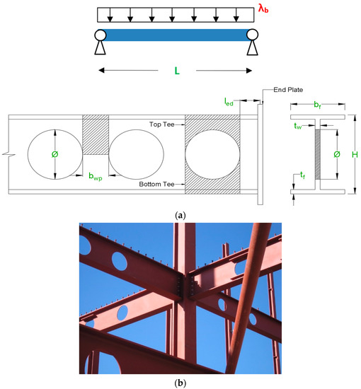
Figure 1.
Steel cellular members: (a) input (parametric) variables, and (b) application in an office building floor system in Lisbon, Portugal.
2.2. Parametric Analysis
The parametric models were submitted to the ABAQUS Lanczos Eigensolver using Python scripts. Table 1 presents the possible values taken for each independent (parametric) variable (see Figure 1a) considered in the FEA. The ‘first’ web opening was placed at the centre of the beam whereas the remaining ones were offset from the former until (for a fixed beam’s length, opening diameter, and web-post width) no more circular openings could fit within member’s length. This approach resulted in 135 different distances from the end opening edge to the centre-line of the endplate (distance named ‘opening-support end distance’ in Table 1). Thus, combining all values of variables 1 and 3 to 8, presented in Table 1, one has (3^6) × 5 lengths = 3645 distinct steel beams for FEA (also called data points or examples in this manuscript). The 3645-point dataset considered in ANN simulations is available in [31].
3. Artificial Neural Networks
3.1. Introduction
Machine learning, one of the six disciplines of artificial intelligence (AI) without which the task of having machines acting humanly could not be accomplished, allows us to ‘teach’ computers how to perform tasks by providing examples of how they should be done [32]. When there is abundant data (also called examples or patterns) explaining a certain phenomenon, but its theory richness is poor, machine learning can be a perfect tool. The world is quietly being reshaped by machine learning, being the artificial neural network (also referred in this manuscript as ANN or neural net) its (i) oldest [33] and (ii) most powerful [34] technique. ANNs also lead the number of practical applications, virtually covering any field of knowledge ([35,36]). In its most general form, an ANN is a mathematical model designed to perform a particular task, based in the way the human brain processes information, i.e. with the help of its processing units (the neurons). ANNs have been employed to perform several types of real-world basic tasks. Concerning functional approximation, ANN-based solutions are frequently more accurate than those provided by traditional approaches, such as multi-variate nonlinear regression, besides not requiring a good knowledge of the function shape being modeled [37].
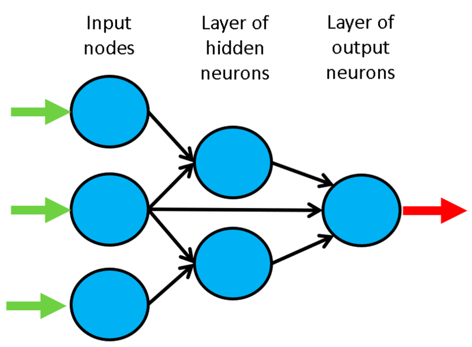
The general ANN structure consists of several nodes disposed in L vertical layers (input layer, hidden layers, and output layer) and connected between them, as depicted in Figure 2. Associated to each node in layers 2 to L, also called neuron, is a linear or nonlinear transfer (also called activation) function, which receives the so-called net input and transmits an output (see Figure 5). All ANNs implemented in this work are called feedforward, since data presented in the input layer flows in the forward direction only, i.e. every node only connects to nodes belonging to layers located at the right-hand-side of its layer, as shown in Figure 2. ANN’s computing power makes them suitable to efficiently solve small to large-scale complex problems, which can be attributed to their (i) massively parallel distributed structure and (ii) ability to learn and generalize, i.e., produce reasonably accurate outputs for inputs not used during the learning (also called training) phase.

Figure 2.
Example of a feedforward neural network.
3.2. Learning
Each connection between 2 nodes is associated to a synaptic weight (real value), which, together with each neuron’s bias (also a real value), are the most common types of neural net unknown parameters that will be determined through learning. Learning is nothing else than determining network unknown parameters through some algorithm in order to minimize network’s performance measure, typically a function of the difference between predicted and target (desired) outputs. When ANN learning has an iterative nature, it consists of three phases: (i) training, (ii) validation, and (iii) testing. From previous knowledge, examples or data points are selected to train the neural net, grouped in the so-called training dataset. Those examples are said to be ‘labelled’ or ‘unlabeled’, whether they consist of inputs paired with their targets, or just of the inputs themselves—learning is called supervised (e.g., functional approximation, classification) or unsupervised (e.g., clustering), whether data used is labelled or unlabeled, respectively. During an iterative learning, while the training dataset is used to tune network unknowns, a process of cross-validation takes place by using a set of data completely distinct from the training counterpart (the validation dataset), so that the generalization performance of the network can be attested. Once ‘optimum’ network parameters are determined, typically associated to a minimum of the validation performance curve (called early stop—see Figure 3), many authors still perform a final assessment of model’s accuracy, by presenting to it a third fully distinct dataset called ‘testing’. Heuristics suggests that early stopping avoids overfitting, i.e. the loss of ANN’s generalization ability. One of the causes of overfitting might be learning too many input-target examples suffering from data noise, since the network might learn some of its features, which do not belong to the underlying function being modeled [38].
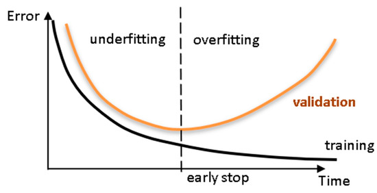
Figure 3.
Cross-validation—assessing network’s generalization ability.
3.3. Implemented ANN features
The ‘behavior’ of any ANN depends on many ‘features’, having been considered 15 ANN features in this work (including data pre/post processing ones). For those features, it is important to bear in mind that no ANN guarantees good approximations via extrapolation (either in functional approximation or classification problems), i.e. the implemented ANNs should not be applied outside the input variable ranges used for network training. Since there are no objective rules dictating which method per feature guarantees the best network performance for a specific problem, an extensive parametric analysis (composed of nine parametric sub-analyses) was carried out to find ‘the optimum’ net design. A description of all implemented methods, selected from state of art literature on ANNs (including both traditional and promising modern techniques), is presented next—Table 2, Table 3 and Table 4 present all features and methods per feature. The whole work was coded in MATLAB [39], making use of its neural network toolbox when dealing with popular learning algorithms (1–3 in Table 4). Each parametric sub-analysis (SA) consists of running all feasible combinations (also called ‘combos’) of pre-selected methods for each ANN feature, in order to get performance results for each designed net, thus allowing the selection of the best ANN according to a certain criterion. The best network in each parametric SA is the one exhibiting the smallest average relative error (called performance) for all learning data.

Table 2.
Implemented artificial neural network (ANN) features (F) 1–5.

Table 3.
Implemented ANN features (F) 6–10.

Table 4.
Implemented ANN features (F) 11–15.
It is worth highlighting that, in this manuscript, whenever a vector is added to a matrix, it means the former is to be added to all columns of the latter (valid in MATLAB).
3.3.1. Qualitative Variable Representation (Feature 1)
A qualitative variable taking n distinct ‘values’ (usually called classes) can be represented in any of the following formats: one variable taking n equally spaced values in [0, 1], or 1-of-n encoding (boolean vectors —e.g., n = 3: [1 0 0] represents class 1, [0 1 0] represents class 2, and [0 0 1] represents class 3). After transformation, qualitative variables are placed at the end of the corresponding (input or output) dataset, in the same original order.
3.3.2. Dimensional Analysis (Feature 2)
The most widely used form of dimensional analysis is the Buckingham’s π-theorem, which was implemented in this work as described in [40].
3.3.3. Input Dimensionality Reduction (Feature 3)
When designing any ANN, it is crucial for its accuracy that the input variables are independent and relevant to the problem ([18,41]). There are two types of dimensionality reduction, namely (i) feature selection (a subset of the original set of input variables is used), and (ii) feature extraction (transformation of initial variables into a smaller set). In this work, dimensionality reduction is never performed when the number of input variables is less than six. The implemented methods are described next.
Linear Correlation
In this feature selection method, all possible pairs of input variables are assessed with respect to their linear dependence, by means of the Pearson correlation coefficient RXY, where X and Y denote any two distinct input variables. For a set of n data points (xi, yi), the Pearson correlation is defined by
where (i) Var(X) and Cov(X, Y) are the variance of X and covariance of X and Y, respectively, and (ii) and are the mean values of each variable. In this work, cases where indicate that one of the variables in the pair must be removed from the ANN modeling. The one to be removed is the one appearing less in the remaining pairs where . Once a variable is selected for removal, all pairs involving it must be disregarded in the subsequent steps for variable removal.
Auto-Encoder
This feature extraction technique uses itself a 3-layer feedforward ANN called auto-encoder (AE). After training, the hidden layer output (y2p) for the presentation of each problem’s input pattern (y1p) is a compressed vector (Q2 x 1) that can be used to replace the original input layer by a (much) smaller one, thus reducing the size of the ANN model. In this work, Q2=round(Q1/2) was adopted, being round a function that rounds the argument to the nearest integer. The implemented AE was trained using the ‘trainAutoencoder(…)’ function from MATLAB’s neural net toolbox. In order to select the best AE, 40 AEs were simulated, and their performance compared by means of the performance variable defined in Section 3.4. Each AE considered distinct (random) initialization parameters, half of the models used the ‘logsig’ hidden transfer functions, and the other half used the ‘satlin’ counterpart, being the identity function the common option for the output activation. In each AE, the maximum number of epochs—number of times the whole training dataset is presented to the network during learning, was defined (regardless the amount of data) by
Concerning the learning algorithm used for all AEs, no L2 weight regularization was employed, which was the only default specification not adopted in ‘trainAutoencoder (…)’.
Orthogonal and Sparse Random Projections
This is another feature extraction technique aiming to reduce the dimension of input data Y1 (Q1 × P) while retaining the Euclidean distance between data points in the new feature space. This is attained by projecting all data along the (i) orthogonal or (ii) sparse random matrix A (Q1 × Q2, Q2 < Q1), as described by Kasun et al. [41].
3.3.4. Training, Validation and Testing Datasets (Feature 4)
Four distributions of data (methods) were implemented, namely pt-pv-ptt = {80-10-10, 70-15-15, 60-20-20, 50-25-25}, where pt-pv-ptt represent the amount of training, validation and testing examples as % of all learning data (P), respectively. Aiming to divide learning data into training, validation and testing subsets according to a predefined distribution pt-pv-ptt, the following algorithm was implemented (all variables are involved in these steps, including qualitative ones after converted to numeric—see Section 3.3.1):
- For each variable q (row) in the complete input dataset, compute its minimum and maximum values.
- Select all patterns (if some) from the learning dataset where each variable takes either its minimum or maximum value. Those patterns must be included in the training dataset, regardless what pt is. However, if the number of patterns ‘does not reach’ pt, one should add the missing amount, providing those patterns are the ones having more variables taking extreme (minimum or maximum) values.
- In order to select the validation patterns, randomly select pv/(pv + ptt) of those patterns not belonging to the previously defined training dataset. The remainder defines the testing dataset.
It might happen that the actual distribution pt-pv-ptt is not equal to the one imposed a priori (before step 1), which is due to the minimum required training patterns specified in step 2.
3.3.5. Input Normalization (Feature 5)
The progress of training can be impaired if training data defines a region that is relatively narrow in some dimensions and elongated in others, which can be alleviated by normalizing each input variable across all data patterns. The implemented techniques are the following:
Linear Max Abs
Lachtermacher and Fuller [42] proposed a simple normalization technique given by
where {Y1}n (i, :) and Y1 (i, :) are the normalized and non-normalized values of the ith input variable for all learning patterns, respectively. Notation ‘:’ in the column index, indicate the selection of all columns (learning patterns).
Linear [0, 1] and [−1, 1]
A linear transformation for each input variable (i), mapping values in Y1(i,:) from [a*, b*] = [min(Y1(i,:)), max(Y1(i,:))] to a generic range [a, b], is obtained from
Ranges [a, b] = [0, 1] and [a, b] = [−1, 1] were considered.
Nonlinear
Proposed by Pu and Mesbahi [43], although in the context of output normalization, the only nonlinear normalization method implemented for input data reads
where (i) Y1(i, j) is the non-normalized value of input variable i for pattern j, (ii) t is the number of digits in the integer part of Y1(i, j), (iii) sign(…) yields the sign of the argument, and (iv) C(i) is the average of two values concerning variable i, C1(i) and C2(i), where the former leads to a minimum normalized value of 0.2 for all patterns, and the latter leads to a maximum normalized value of 0.8 for all patterns.
Linear Mean Std
Tohidi and Sharifi [20] proposed the following technique
where and are the mean and standard deviation of all non-normalized values (all patterns) stored by variable i.
3.3.6. Output Transfer Functions (Feature 6)
Logistic
The most usual form of transfer functions is called Sigmoid. An example is the logistic function given by
Hyperbolic Tang
The Hyperbolic Tangent function is also of sigmoid type, being defined as
Bilinear
The implemented Bilinear function is defined as
Identity
The Identity activation is often employed in output neurons, reading
3.3.7. Output Normalization (Feature 7)
Normalization can also be applied to the output variables so that, for instance, the amplitude of the solution surface at each variable is the same. Otherwise, training may tend to focus (at least in the earlier stages) on the solution surface with the greatest amplitude [44]. Normalization ranges not including the zero value might be a useful alternative since convergence issues may arise due to the presence of many small (close to zero) target values [45]. Four normalization methods were implemented. The first three follow Equation (4), where (i) [a, b] = 70% [φmin, φmax], (ii) [a, b] = 60% [φmin, φmax], and (iii) [a, b] = 50% [φmin, φmax], being [φmin, φmax] the output transfer function range, and [a, b] determined to be centered within [φmin, φmax] and to span the specified % (e.g., (b − a) = 0.7 (φmax − φmin)). Whenever the output transfer functions are unbounded (Bilinear and Identity), it was considered [a, b] = [0, 1] and [a, b] = [−1, 1], respectively. The fourth normalization method implemented is the one described by Equation (6).
3.3.8. Network Architecture (Feature 8)
Multi-Layer Perceptron Network (MLPN)
This is a feedforward ANN exhibiting at least one hidden layer. Figure 2 depicts a 3-2-1 MLPN (3 input nodes, 2 hidden neurons and 1 output neuron), where units in each layer link only to some nodes located ahead. At this moment, it is appropriate to define the concept of partially- (PC) and fully-connected (FC) ANNs. In this work a FC feedforward network is characterized by having each node connected to every node in a different layer placed forward—any other type of network is said to be PC (e.g., the one in Figure 2). According to Wilamowski [46], PC MLPNs are less powerful than MLPN where connections across layers are allowed, which usually lead to smaller networks (less neurons).
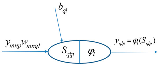
Figure 4 represents a generic MLFN composed of L layers, where l (l = 1,…, L) is a generic layer and ‘ql’ a generic node, being q = 1,…, Ql its position in layer l (1 is reserved to the top node). Figure 5 represents the model of a generic neuron (l = 2,…, L), where (i) p represents the data pattern presented to the network, (ii) subscripts m = 1,…, Qn and n = 1,…, l − 1 are summation indexes representing all possible nodes connecting to neuron ‘ql’ (recall Figure 4), (iii) bql is neuron’s bias, and (iv) wmnql represents the synaptic weight connecting units ‘mn’ and ‘ql’. Neuron’s net input for the presentation of pattern p (Sqlp) is defined as
where ym1p is the value of the mth network input concerning example p. The output of a generic neuron can then be written as (l = 2,…, L)
where φl is the transfer function used for all neurons in layer l.
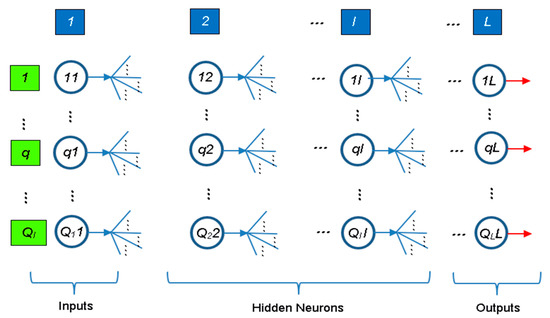
Figure 4.
Generic multi-layer feedforward network.
Radial-Basis Function Network (RBFN)
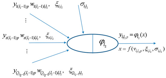
Although having similar topologies, RBFN and MLPN behave very differently due to distinct hidden neuron models—unlike the MLPN, RBFN have hidden neurons behaving differently than output neurons. According to Xie et al. [47], RBFN (i) are specially recommended in functional approximation problems when the function surface exhibits regular peaks and valleys, and (ii) perform more robustly than MLPN when dealing with noisy input data. Although traditional RBFN have 3 layers, a generic multi-hidden layer (see Figure 4) RBFN is allowed in this work, being the generic hidden neuron’s model concerning node ‘l1l2’ (l1 = 1,…,Ql2, l2 = 2,…, L − 1) presented in Figure 6. In this model, (i) and (called RBF center) are vectors of the same size ( denotes de z component of vector , and it is a network unknown), being the former associated to the presentation of data pattern p, (ii) is called RBF width (a positive scalar) and also belongs, along with synaptic weights and RBF centers, to the set of network unknowns to be determined through learning, (iii) is the user-defined radial basis (transfer) function (RBF), described in Equations (20)–(23), and (iv) is neuron’s output when pattern p is presented to the network. In ANNs not involving learning algorithms 1–3 in Table 4, vectors and are defined as (two versions of where implemented and the one yielding the best results was selected)
whereas the RBFNs implemented through MATLAB neural net toolbox (involving learning algorithms 1–3 in Table 4) are based on the following definitions
Lastly, according to the implementation carried out for initialization purposes (described in Section 3.3.12), (i) RBF center vectors per hidden layer (one per hidden neuron) are initialized as integrated in a matrix (termed RBF center matrix) having the same size of a weight matrix linking the previous layer to that specific hidden layer, and (ii) RBF widths (one per hidden neuron) are initialized as integrated in a vector (called RBF width vector) with the same size of a hypothetic bias vector.
3.3.9. Hidden Nodes (Feature 9)
Inspired by several heuristics found in the literature for the determination of a suitable number of hidden neurons in a single hidden layer net ([48,49,50]), each value in hntest, defined in Equation (15), was tested in this work as the total number of hidden nodes in the model, ie the sum of nodes in all hidden layers (initially defined with the same number of neurons). The number yielding the smallest performance measure for all patterns (as defined in Section 3.4, with outputs and targets not postprocessed), is adopted as the best solution. The aforementioned hntest is defined by
where (i) Q1 and QL are the number of input and output nodes, respectively, (ii) P and Pt are the number of learning and training patterns, respectively, and (iii) F13 is the number of feature 13’s method (see Table 4).
3.3.10. Connectivity (Feature 10)
For this ANN feature, three methods were implemented, namely (i) adjacent layers—only connections between adjacent layers are made possible, (ii) adjacent layers + input-output—only connections between (ii1) adjacent and (ii2) input and output layers are allowed, and (iii) fully-connected (all possible feedforward connections).
3.3.11. Hidden Transfer Functions (Feature 11)
Besides functions (i) Logistic—Equation (7), (ii) Hyperbolic Tangent—Equation (8), and (iii) Bilinear—Equation (9), defined in Section 3.3.6, the ones defined next were also implemented as hidden transfer functions. During software validation it was observed that some hidden node outputs could be infinite or NaN (not-a-number in MATLAB—e.g., 0/0 = Inf/Inf = NaN), due to numerical issues concerning some hidden transfer functions and/or their calculated input. In those cases, it was decided to convert infinite to unitary values and NaNs to zero (the only exception was the bipolar sigmoid function, where NaNs were converted to −1). Other implemented trick was to convert possible Gaussian function’s NaN inputs to zero.
Identity-Logistic
In [51], issues associated with flat spots at the extremes of a sigmoid function were eliminated by adding a linear function to the latter, reading
Bipolar
The so-called bipolar sigmoid activation function mentioned in [52], ranging in [−1, 1], reads
Positive Saturating Linear
In MATLAB neural net toolbox, the so-called Positive Saturating Linear transfer function, ranging in [0, 1], is defined as
Sinusoid
Concerning less popular transfer functions, reference is made in [53] to the sinusoid, which in this work was implemented as
Radial Basis Functions (RBF)
Although Gaussian activation often exhibits desirable properties as a RBF, several authors (e.g., [54]) have suggested several alternatives. Following nomenclature used in Section 3.3.8, (i) the Thin-Plate Spline function is defined by
(ii) the next function is employed as Gaussian-type function when learning algorithms 4–7 are used (see Table 4)
(iii) the Multiquadratic function is given by
and (iv) the Gaussian-type function (called ‘radbas’ in MATLAB toolbox) used by RBFNs trained with learning algorithms 1–3 (see Table 4), is defined by
where || … || denotes the Euclidean distance in all functions.
3.3.12. Parameter Initialization (Feature 12)
The initialization of (i) weight matrices (Qa × Qb, being Qa and Qb node numbers in layers a and b being connected, respectively), (ii) bias vectors (Qb × 1), (iii) RBF center matrices (Qc-1 × Qc, being c the hidden layer that matrix refers to), and (iv) RBF width vectors (Qc × 1), are independent and in most cases randomly generated. For each ANN design carried out in the context of each parametric analysis combo, and whenever the parameter initialization method is not the ‘Mini-Batch SVD’, ten distinct simulations varying (due to their random nature) initialization values are carried out, in order to find the best solution. The implemented initialization methods are described next.
Midpoint, Rands, Randnc, Randnr, Randsmall
These are all MATLAB built-in functions. Midpoint is used to initialize weight and RBF center matrices only (not vectors). All columns of the initialized matrix are equal, being each entry equal to the midpoint of the (training) output range leaving the corresponding initial layer node—recall that in weight matrices, columns represent each node in the final layer being connected, whereas rows represent each node in the initial layer counterpart. Rands generates random numbers with uniform distribution in [−1, 1]. Randnc (only used to initialize matrices) generates random numbers with uniform distribution in [−1, 1], and normalizes each array column to 1 (unitary Euclidean norm). Randnr (only used to initialize matrices) generates random numbers with uniform distribution in [−1, 1], and normalizes each array row to 1 (unitary Euclidean norm). Randsmall generates random numbers with uniform distribution in [−0.1, 0.1].
Rand [−lim, lim]
This function is based on the proposal in [55], and generates random numbers with uniform distribution in [−lim, lim], being lim layer-dependent and defined by
where a and b refer to the initial and final layers integrating the matrix being initialized, and L is the total number of layers in the network. In the case of a bias or RBF width vector, lim is always taken as 0.5.
SVD
Although Deng et al. [56] proposed this method for a 3-layer network, it was implemented in this work regardless the number of hidden layers.
Mini-Batch SVD
Based on [56], this scheme is an alternative version of the former SVD. Now, training data is split into min{Qb, Pt} chunks (or subsets) of equal size Pti = max{floor(Pt/Qb), 1}—floor rounds the argument to the previous integer (whenever it is decimal) or yields the argument itself, being each chunk aimed to derive Qbi = 1 hidden node.
3.3.13. Learning Algorithm (Feature 13)
The most popular learning algorithm is called error back-propagation (BP), a first-order gradient method. Second-order gradient methods are known to have higher training speed and accuracy [57]. The most employed is called Levenberg-Marquardt (LM). All these traditional schemes were implemented using MATLAB toolbox [39].
Back-Propagation (BP, BPA), Levenberg-Marquardt (LM)
Two types of BP schemes were implemented, one with constant learning rate (BP)—’traingd’ in MATLAB, and another with iteration-dependent rate, named BP with adaptive learning rate (BPA)—‘traingda’ in MATLAB. The learning parameters set different than their default values are:
- (i)
- Learning Rate = 0.01/cs0.5, being cs the chunk size, as defined in Section 3.3.15.
- (ii)
- Minimum performance gradient = 0.
Concerning the LM scheme—‘trainlm’ in MATLAB, the only learning parameter set different than its default value was the abovementioned (ii).
Extreme Learning Machine (ELM, mb ELM, I-ELM, CI-ELM)
Besides these traditional learning schemes, iterative and time-consuming by nature, four versions of a recent, powerful and non-iterative learning algorithm, called Extreme Learning Machine (ELM), were implemented (unlike initially proposed by the authors of ELM, connections across layers were allowed in this work), namely: (batch) ELM [58], Mini-Batch ELM (mb ELM) [59], Incremental ELM (I-ELM) [60], Convex Incremental ELM (CI-ELM) [61].
3.3.14. Performance Improvement (Feature 14)
A simple and recursive approach aiming to improve ANN accuracy is called Neural Network Composite (NNC), as described in [62]. In this work, a maximum of 10 extra ANNs were added to the original one, until maximum error was not improved between successive NNC solutions. Later in this manuscript, a solution given by a single neural net might be denoted as ANN, whereas the other possible solution is called NNC.
3.3.15. Training Mode (Feature 15)
Depending on the relative amount of training patterns, with respect to the whole training dataset, that is presented to the network in each iteration of the learning process, several types of training modes can be used, namely (i) batch or (ii) mini-batch. Whereas in the batch mode all training patterns are presented (called an epoch) to the network in each iteration, in the mini-batch counterpart the training dataset is split into several data chunks (or subsets) and in each iteration a single and new chunk is presented to the network, until (eventually) all chunks have been presented. Learning involving iterative schemes (e.g., BP- or LM-based) might require many epochs until an ‘optimum’ design is found. The particular case of having a mini-batch mode where all chunks are composed by a single (distinct) training pattern (number of data chunks = Pt, chunk size = 1), is called online or sequential mode. Wilson and Martinez [63] suggested that if one wants to use mini-batch training with the same stability as online training, a rough estimate of the suitable learning rate to be used in learning algorithms such as the BP, is ηonline /, where cs is the chunk size and ηonline is the online learning rate—their proposal was adopted in this work. Based on the proposal of Liang et al. [59], the constant chunk size (cs) adopted for all chunks in mini-batch mode reads cs = min{mean(hn) + 50, Pt}, being hn a vector storing the number of hidden nodes in each hidden layer in the beginning of training, and mean(hn) the average of all values in hn.
3.4. Network Performance Assessment
Several types of results were computed to assess network outputs, namely (i) maximum error, (ii) % errors greater than 3%, and (iii) performance, which are defined next. All above-mentioned errors are relative errors (expressed in %) based on the following definition, concerning a single output variable and data pattern,
where (i) dqp is the qth desired (or target) output when pattern p within iteration i (p = 1,…, Pi) is presented to the network, and (ii) yqLp is net’s qth output for the same data pattern. Moreover, denominator in Equation (25) is replaced by 1 whenever |dqp| < 0.05 − dqp in the nominator keeps its real value. This exception to Equation (25) aims to reduce the apparent negative effect of large relative errors associated to target values close to zero. Even so, this trick may still lead to (relatively) large solution errors while groundbreaking results are depicted as regression plots (target versus predicted outputs).
3.4.1. Maximum Error
This variable measures the maximum relative error, as defined by Equation (25), among all output variables and learning patterns.
3.4.2. Percentage of Errors > 3%
This variable measures the percentage of relative errors, as defined by Equation (25), among all output variables and learning patterns, that are greater than 3%.
3.4.3. Performance
In functional approximation problems, network performance is defined as the average relative error, as defined in Equation (25), among all output variables and data patterns being evaluated (e.g., training, all data).
3.5. Software Validation
Several benchmark datasets/functions were used to validate the developed software, involving low- to high-dimensional problems and small to large volumes of data. Due to paper length limit, validation results are not presented herein but they were made public in [64].
3.6. Parametric Analysis Results
Aiming to reduce the computing time by cutting in the number of combos to be run—note that all features combined lead to hundreds of millions of combos, the whole parametric simulation was divided into nine parametric SAs, where in each one feature 7 only takes a single value. This measure aims to make the performance ranking of all combos within each ‘small’ analysis more ‘reliable’, since results used for comparison are based on target and output datasets as used in ANN training and yielded by the designed network, respectively (they are free of any postprocessing that eliminates output normalization effects on relative error values). Whereas (i) the 1st and 2nd SAs aimed to select the best methods from features 1, 2, 5, 8, and 13 (all combined), while adopting a single popular method for each of the remaining features (F3: 6, F4: 2, F6: {1 or 7}, F7: 1, F9: 1, F10: 1, F11: {3, 9 or 11}, F12: 2, F14: 1, F15: 1—see Table 2, Table 3 and Table 4)—SA 1 involved learning algorithms 1–3 and SA 2 involved the ELM-based counterpart, (ii) the 3rd–7th SAs combined all possible methods from features 3, 4, 6, and 7, and concerning all other features, adopted the methods integrating the best combination from the aforementioned first SA, (iii) the 8th SA combined all possible methods from features 11, 12, and 14, and concerning all other features, adopted the methods integrating the best combination (results compared after postprocessing) among the previous five sub-analyses, and lastly (iv) the 9th SA combined all possible methods from features 9, 10 and 15, and concerning all other features, adopted the methods integrating the best combination from the previous analysis. Summing up the ANN feature combinations for all parametric SAs, a total of 475 combos were run for this work.
ANN feature methods used in the best combo from each of the abovementioned nine parametric sub-analyses, are specified in Table 5 (the numbers represent the method number as in Table 2, Table 3 and Table 4). Table 6 shows the corresponding relevant results for those combos, namely (i) maximum error, (ii) % errors > 3%, (iii) performance (all described in Section 3, and evaluated for all learning data), (iv) total number of hidden nodes in the model, and (v) average computing time per example (including data pre- and post-processing). All results shown in Table 6 are based on target and output datasets computed in their original format, i.e. free of any transformations due to output normalization and/or dimensional analysis. The microprocessors used in this work have the following features: OS: Win10Home 64bits, RAMs: 48/128 GB, Local Disk Memory: 1 TB, CPUs: Intel® Core™ i7 8700K @ 3.70–4.70 GHz/i9 7960X @ 2.80-4.20 GHz.

Table 5.
ANN feature (F) methods used in the best combo from each parametric sub-analysis (SA).

Table 6.
Performance results for the best design from each parametric sub-analysis: (a) ANN, (b) NNC.
3.7. Proposed ANN-Based Model
The proposed model is the one, among the best ones from all parametric SAs, exhibiting the lowest maximum error (SA 9). That model is characterized by the ANN feature methods {1, 2, 1, 3, 1, 7, 5, 1, 3, 3, 1, 5, 3, 1, 3} in Table 2, Table 3 and Table 4. Aiming to allow implementation of this model by any user, all variables/equations required for (i) data preprocessing, (ii) ANN simulation, and (iii) data postprocessing, are presented in Section 3.7.1, Section 3.7.2 and Section 3.7.3, respectively. The proposed model is a single MLPN with 5 layers and a distribution of nodes/layer of 8-11-11-11-1. Concerning connectivity, the network is fully-connected, and the hidden and output transfer functions are all Logistic (Equation (7)) and Identity (Equation (10)), respectively. The network was trained using the LM algorithm (1500 epochs). After design, the average network computing time concerning the presentation of a single example (including data pre/postprocessing) is 6.93 × 10⁻⁵ s—Figure 7 depicts a simplified scheme of some of network key features. Lastly, all relevant performance results concerning the proposed ANN are illustrated in Section 3.7.4. The obtained ANN solution for every data point can be found in [31].

Figure 7.
Proposed 8-11-11-11-1 fully-connected MLPN—simplified scheme.
It is worth recalling that, in this manuscript, whenever a vector is added to a matrix, it means the former is to be added to all columns of the latter (valid in MATLAB).
3.7.1. Input Data Preprocessing
For future use of the proposed ANN to simulate new data Y1,sim (8 × Psim matrix) concerning Psim patterns, the same data preprocessing (if any) performed before training must be applied to the input dataset. That preprocessing is defined by the methods used for ANN features 2, 3 and 5 (respectively 2, 6 and 1—see Table 2), which should be applied after all (eventual) qualitative variables in the input dataset are converted to numerical (using feature 1’s method). Next, the necessary preprocessing to be applied to Y1,sim, concerning features 2, 3 and 5, is fully described.
Dimensional Analysis and Dimensionality Reduction
Since dimensional analysis (d.a.) and dimensionality reduction (d.r.) were not carried out, one has
Input Normalization
After input normalization, the new input dataset is defined as function of the previously determined , and they have the same size, reading
where one recalls that operator ‘.x’ multiplies component i in vector INP by all components in row i of .
3.7.2. ANN-Based Analytical Model
Once determined the preprocessed input dataset {Y1,sim}nafter(8 × Psim matrix), the next step is to present it to the proposed ANN to obtain the predicted output dataset {Y5,sim}nafter (1 × Psim vector), which will be given in the same preprocessed format of the target dataset used in learning. In order to convert the predicted outputs to their ‘original format’ (i.e., without any transformation due to normalization or dimensional analysis—the only transformation visible will be the (eventual) qualitative variables written in their numeric representation), some postprocessing is needed, as described in detail in Section 3.7.3. Next, the mathematical representation of the proposed ANN is given, so that any user can implement it to determine {Y5,sim}nafter, thus eliminating all rumors that ANNs are ‘black boxes’.
where
Arrays Wj-s and bs are stored online in [65], aiming to avoid an overlong article and ease model’s implementation by any interested reader.
3.7.3. Output Data Postprocessing
In order to transform the output dataset obtained by the proposed ANN, {Y5,sim}nafter (1 × Psim vector), to its original format (Y5,sim), i.e. without the effects of dimensional analysis and/or output normalization (possibly) taken in target dataset preprocessing prior training, the postprocessing addressed next must be performed.
Once obtained {Y5,sim}nafter, the following relations hold for its relation to its non-normalized () and original (Y5,sim) formats (just after the dimensional analysis stage, and free of any pre-processing effects, respectively), reading
since no output normalization nor dimensional analysis were carried out.
3.7.4. Performance Results
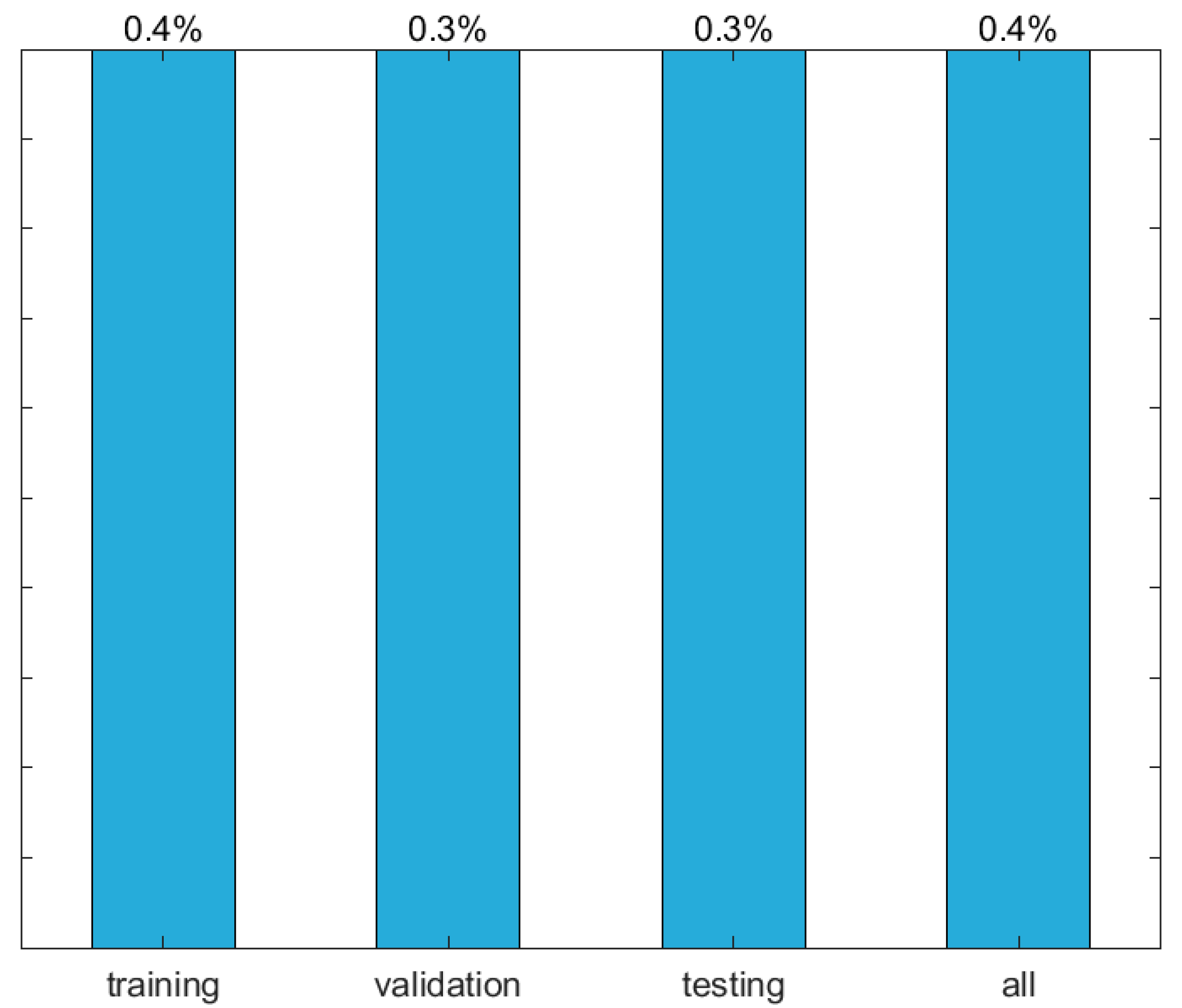
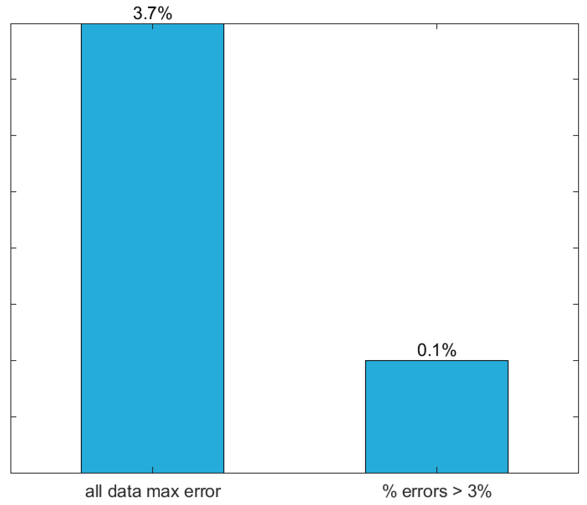
Finally, results yielded by the proposed ANN, in terms of performance variables defined in Section 3.4, are presented in this section in the form of several graphs: (i) a regression plot per output variable (Figure 8), where network target and output data are plotted, for each data point, as x- and y- coordinates, respectively—a measure of quality is given by the Pearson Correlation Coefficient (R), as defined in Equation (1); (ii) a performance plot (Figure 9), where performance (average error) values are displayed for several learning datasets; and (iii) an error plot (Figure 10), where values concern all data (iii1) maximum error and (iii2) % of errors greater than 3%. It is worth highlighting that all graphical results just mentioned are based on effective target and output values, i.e. computed in their original format.
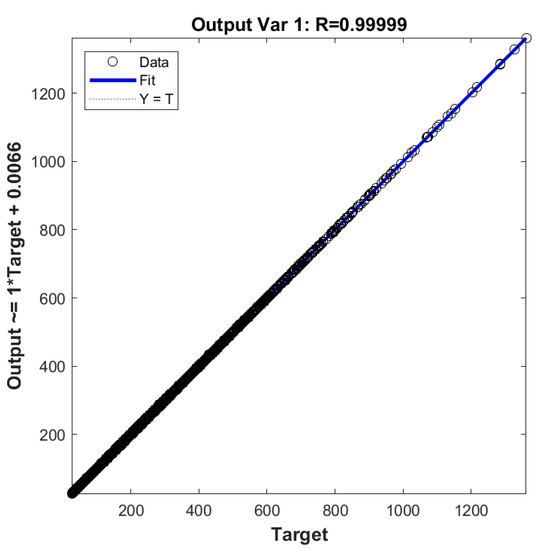
Figure 8.
Regression plot for the proposed ANN.
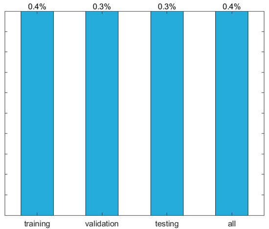
Figure 9.
Performance plot (mean errors) for the proposed ANN.

Figure 10.
Error plot for the proposed ANN.
4. Design Considerations
The bar chart in Figure 11, where beams numbers in the horizontal axis are referenced to the data point ID in the ANN dataset [31], presents (i) the design loads given by SCI-P355 [15], and (ii) the FEA-based elastic buckling loads obtained from this work. As expected, SCI-P355 yielded significantly lower loads and it is worth noting that the differences between the two approaches do not produce the same percentage variance in load estimates for the 8 randomly selected beams. In particular, for slender web-posts (i.e., closely spaced web openings) such as in beams 82, 136, 163, and 217, buckling of the web-post will always govern the design in SCI-P355, hence the reduced design load. As for the FEAs, parameter led (end web-post distance to the support—see Figure 1a) governs the design for widely spaced web openings. SCI-P355 does not consider the distance led and recommends it to be greater than 50% of the opening diameter. In this work, the opening diameter and web-post width were taken within the recommended design limits (1.25 < H/Φ < 1.75 and 1.08 < (bwp + Φ)/Φ < 1.5, respectively).
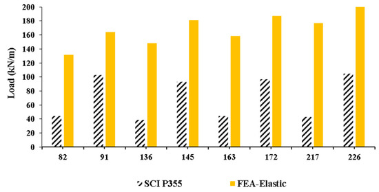
Figure 11.
SCI P355 design strength versus FE-based elastic buckling prediction.
5. Concluding Remarks
An ANN-based analytical model is proposed to effectively predict the elastic buckling load of simply supported cellular steel beams subjected to a uniformly distributed load. Finite element solutions from 3645 distinct beams were used for ANN design (training, validation, and testing). The independent variables adopted as ANN inputs are the following: beam’s length, opening diameter, web-post width, cross-section height, web thickness, flange width, flange thickness, and the distance between the last opening edge and the end support. The maximum and average relative errors yielded by the proposed ANN among the 3645 data points were 3.7% and 0.4%, respectively. Moreover, that model is able to compute the buckling load of a single beam in less than a millisecond, for any current personal computer. These facts make the proposed model a potential tool for structural engineers and researchers who aim to accurately estimate the elastic buckling load of cellular steel beams (i) within the ranges of the input variables adopted in this study (see Table 1), and (ii) without the burden of the costly resources associated to FEA.
This research is the first step of an ongoing investigation that aims to propose a novel and simple analytical design method to accurately compute the inelastic resistance of cellular steel beams.
Author Contributions
Conceptualization, M.A.; Methodology, M.A.; Software, M.A.; Data Curation, K.R., K.D.T.; Writing-Original Draft Preparation, M.A., K.R., K.D.T., T.P.R.; Writing-Review & Editing, M.A., K.R., K.D.T., T.P.R.
Funding
This research received no external funding.
Acknowledgments
The authors would like to thank the UK Research Council (EPSRC: EP/L504993/1) and the University of Leeds for their financial support.
Conflicts of Interest
The authors declare no conflict of interest.
References
- Tsavdaridis, K.D. Structural Performance of Perforated Steel Beams with Novel Web Openings and with Partial Concrete Encasement. Ph.D. Thesis, City University of London, London, UK, 2010. [Google Scholar]
- Morkhade, S.G.; Gupta, L.M. An experimental and parametric study on steel beams with web openings. Int. J. Adv. Struct. Eng. 2015, 7, 249–260. [Google Scholar] [CrossRef]
- Akrami, V.; Erfani, S. Review and assessment of design methodologies for perforated steel beams. J. Struct. Eng. 2016, 142, 1–14. [Google Scholar] [CrossRef]
- Uenoya, M.; Redwood, R.G. Buckling of webs with openings. Comput. Struct. 1978, 9, 191–199. [Google Scholar] [CrossRef]
- Lucas, W.K.; Darwin, D. Steel and Composite Beams with Web Openings; The American Iron and Steel Institute: City of Wichita, KS, USA, 1990. [Google Scholar]
- Darwin, D. Steel and Composite Beams with Web Opening; Steel Design Guide Series 2; American Institute of Steel Construction (AISC): Chicago, IL, USA, 1990. [Google Scholar]
- SEI/ASCE. Specifications for Structural Steel Beams with Openings; SEI/ASCE 23-97; ASCE: Reston, VA, USA, 1998. [Google Scholar]
- Ward, J.K. Design of Composite and Non-Composite Cellular Beams SCI P100; Steel Construction Institute: Berkshire, UK, 1990. [Google Scholar]
- Chung, K.F.; Lui, T.C.H.; Ko, A.C.H. Investigation on vierendeel mechanism in steel beams with circular web openings. J. Constr. Steel Res. 2001, 57, 467–490. [Google Scholar] [CrossRef]
- Chung, K.F.; Liu, C.H.; Ko, A.C.H. Steel beams with large web openings of various shapes and sizes: An empirical design method using a generalized moment-shear interaction curve. J. Constr. Steel Res. 2003, 59, 1177–1200. [Google Scholar] [CrossRef]
- Tsavdaridis, K.D.; D’Mello, C. Finite Element Investigation of Perforated Beams with Different Web Opening Configurations. In Proceedings of the 6th International Conference on Advances is Steel Structures (ICASS 2009), Hong Kong, China, 16–18 December 2009; pp. 213–220. [Google Scholar]
- Tsavdaridis, K.D.; D’Mello, C. Web buckling study of the behaviour and strength of perforated steel beams with different novel web opening shapes. J. Constr. Steel Res. 2011, 67, 1605–1620. [Google Scholar] [CrossRef]
- Tsavdaridis, K.D.; D’Mello, C. Vierendeel bending study of perforated steel beams with various novel web opening shapes through non-linear finite element analyses. J. Struct. Eng. 2012, 138, 1214–1230. [Google Scholar] [CrossRef]
- Tsavdaridis, K.D.; Kingman, J.J.; Toropov, V.V. Application of Structural Topology Optimisation to Perforated Steel Beams. Comput. Struct. 2015, 158, 108–123. [Google Scholar] [CrossRef]
- Lawson, R.M.; Hicks, S.J. Design of Composite Beams with Large Openings SCI P355; Steel Construction Institute: Berkshire, UK, 2011. [Google Scholar]
- Lawson, R.M. Design for Openings in the Webs of Composite Beams SCI P068; Steel Construction Institute: Berkshire, UK, 1987. [Google Scholar]
- Verweij, J.G. Cellular Beam-Columns in Portal Frame Structures. Master’s Thesis, Delft University of Technology, Delft, The Netherlands, 2010. [Google Scholar]
- Gholizadeh, S.; Pirmoz, A.; Attarnejad, R. Assessment of load carrying capacity of castellated steel beams by neural networks. J. Constr. Steel Res. 2011, 67, 770–779. [Google Scholar] [CrossRef]
- Sharifi, Y.; Tohidi, S. Lateral-torsional buckling capacity assessment of web opening steel girders by artificial neural networks—Elastic investigation. Front. Struct. Civ. Eng. 2014, 8, 167–177. [Google Scholar] [CrossRef]
- Tohidi, S.; Sharifi, Y. Inelastic lateral-torsional buckling capacity of corroded web opening steel beams using artificial neural networks. IES J. Part A Civ. Struct. Eng. 2014, 8, 24–40. [Google Scholar] [CrossRef]
- Tohidi, S.; Sharifi, Y. Load-carrying capacity of locally corroded steel plate girder ends using artificial neural network. Thin-Walled Struct. 2016, 100, 48–61. [Google Scholar] [CrossRef]
- Asteris, P.G.; Kolovos, K.G.; Douvika, M.G.; Roinos, K. Prediction of self-compacting concrete strength using artificial neural networks. Eur. J. Environ. Civ. Eng. 2016, 20 (Suppl. 1), S102–S122. [Google Scholar] [CrossRef]
- Cascardi, A.; Micelli, F.; Aiello, M.A. An Artificial Neural Networks model for the prediction of the compressive strength of FRP-confined concrete circular columns. Eng. Struct. 2017, 140, 199–208. [Google Scholar] [CrossRef]
- Marović, I.; Androjić, I.; Jajac, N.; Hanák, T. Urban Road Infrastructure Maintenance Planning with Application of Neural Networks. Complexity 2018, 2018, 1–10. [Google Scholar] [CrossRef]
- Wong, E.W.C.; Choi, H.S.; Kim, D.K.; Hashim, F.M. Development of ANN Model for the Prediction of VIV Fatigue Damage of Top-tensioned Riser. MATEC Web Conf. 2018, 203, 1013. [Google Scholar] [CrossRef]
- Dassault Systèmes. ABAQUS 6.11, Abaqus/CAE User’s Manual; Dassault Systemes: Vélizy-Villacoublay, France, 2011. [Google Scholar]
- Dassault Systèmes Simulia Corp. ABAQUS CAE (2017); Software; Dassault Systèmes Simulia Corp.: Vélizy-Villacoublay, France, 2017. [Google Scholar]
- Surtees, J.O.; Lui, Z. Report of Loading Tests on Cellform Beams; Research Report; University of Leeds: Leeds, UK, 1995. [Google Scholar]
- Rajana, K. Advanced Computational Parametric Study of the Linear Elastic and Non-Linear Post Buckling Behaviour of Non-Composite Cellular Steel Beams. Master’s Thesis, University of Leeds, Leeds, UK, 2018. [Google Scholar] [CrossRef]
- El-Sawhy, K.L.; Sweedan, A.M.I.; Martini, M.I. Moment gradient factor of cellular steel beams under inelastic flexure. J. Constr. Steel Res. 2014, 98, 20–34. [Google Scholar] [CrossRef]
- Developer. Dataset ANN [Data Set]. Zenodo. 2018. Available online: http://doi.org/10.5281/zenodo.1486181 (accessed on 29 November 2018).
- Hertzmann, A.; Fleet, D. Machine Learning and Data Mining; Lecture Notes CSC 411/D11; Computer Science Department, University of Toronto: Toronto, ON, Canada, 2012. [Google Scholar]
- McCulloch, W.S.; Pitts, W. A logical calculus of the ideas immanent in nervous activity. Bull. Math. Biophys. 1943, 5, 115–133. [Google Scholar] [CrossRef]
- Hern, A. Google Says Machine Learning Is the Future. So I Tried It Myself. Available online: www.theguardian.com/technology/2016/jun/28/all (accessed on 2 November 2016).
- Prieto, A.; Prieto, B.; Ortigosa, E.M.; Ros, E.; Pelayo, F.; Ortega, J.; Rojas, I. Neural networks: An overview of early research, current frameworks and new challenges. Neurocomputing 2016, 214, 242–268. [Google Scholar] [CrossRef]
- Wilamowski, B.M.; Irwin, J.D. The Industrial Electronics Handbook: Intelligent Systems; CRC Press: Boca Raton, FL, USA, 2011. [Google Scholar]
- Flood, I. Towards the next generation of artificial neural networks for civil engineering. Adv. Eng. Inform. 2008, 228, 4–14. [Google Scholar] [CrossRef]
- Haykin, S.S. Neural Networks and Learning Machines; Prentice Hall/Pearson: New York, NY, USA, 2009. [Google Scholar]
- The Mathworks, Inc. MATLAB R2017a, User’s Guide; The Mathworks, Inc.: Natick, MA, USA, 2017. [Google Scholar]
- Bhaskar, R.; Nigam, A. Qualitative physics using dimensional analysis. Artif. Intell. 1990, 45, 111–173. [Google Scholar] [CrossRef]
- Kasun, L.L.C.; Yang, Y.; Huang, G.-B.; Zhang, Z. Dimension reduction with extreme learning machine. IEEE Trans. Image Process. 2016, 25, 3906–3918. [Google Scholar] [CrossRef] [PubMed]
- Lachtermacher, G.; Fuller, J.D. Backpropagation in time-series forecasting. J. Forecast. 1995, 14, 381–393. [Google Scholar] [CrossRef]
- Pu, Y.; Mesbahi, E. Application of artificial neural networks to evaluation of ultimate strength of steel panels. Eng. Struct. 2006, 28, 1190–1196. [Google Scholar] [CrossRef]
- Flood, I.; Kartam, N. Neural Networks in Civil Engineering: I-Principals and Understanding. J. Comput. Civ. Eng. 1994, 8, 131–148. [Google Scholar] [CrossRef]
- Mukherjee, A.; Deshpande, J.M.; Anmala, J. Prediction of buckling load of columns using artificial neural networks. J. Struct. Eng. 1996, 122, 1385–1387. [Google Scholar] [CrossRef]
- Wilamowski, B.M. Neural Network Architectures and Learning algorithms. IEEE Ind. Electron. Mag. 2009, 3, 56–63. [Google Scholar] [CrossRef]
- Xie, T.; Yu, H.; Wilamowski, B. Comparison between traditional neural networks and radial basis function networks. In Proceedings of the 2011 IEEE International Symposium on Industrial Electronics (ISIE), Gdansk University of Technology Gdansk, Gdansk, Poland, 27–30 June 2011; pp. 1194–1199. [Google Scholar]
- Aymerich, F.; Serra, M. Prediction of fatigue strength of composite laminates by means of neural networks. Key Eng. Mater. 1998, 144, 231–240. [Google Scholar] [CrossRef]
- Rafiq, M.; Bugmann, G.; Easterbrook, D. Neural network design for engineering applications. Comput. Struct. 2001, 79, 1541–1552. [Google Scholar] [CrossRef]
- Xu, S.; Chen, L. Novel approach for determining the optimal number of hidden layer neurons for FNN’s and its application in data mining. In Proceedings of the International Conference on Information Technology and Applications (ICITA), Cairns, Australia, 23–26 June 2008; pp. 683–686. [Google Scholar]
- Gunaratnam, D.J.; Gero, J.S. Effect of representation on the performance of neural networks in structural engineering applications. Comput.-Aided Civ. Infrastruct. Eng. 1994, 9, 97–108. [Google Scholar] [CrossRef]
- Lefik, M.; Schrefler, B.A. Artificial neural network as an incremental non-linear constitutive model for a finite element code. Comput. Methods Appl. Mech. Eng. 2003, 192, 3265–3283. [Google Scholar] [CrossRef]
- Bai, Z.; Huang, G.; Wang, D.; Wang, H.; Westover, M. Sparse extreme learning machine for classification. IEEE Trans. Cybern. 2014, 44, 1858–1870. [Google Scholar] [CrossRef] [PubMed]
- Schwenker, F.; Kestler, H.; Palm, G. Three learning phases for radial-basis-function networks. Neural Netw. 2001, 14, 439–458. [Google Scholar] [CrossRef]
- Waszczyszyn, Z. Neural Networks in the Analysis and Design of Structures; CISM Courses and Lectures No. 404; Springer: Wien, Austria; New York, NY, USA, 1999. [Google Scholar]
- Deng, W.-Y.; Bai, Z.; Huang, G.-B.; Zheng, Q.-H. A fast SVD-Hidden-nodes based extreme learning machine for large-scale data Analytics. Neural Netw. 2016, 77, 14–28. [Google Scholar] [CrossRef]
- Wilamowski, B.M. How to not get frustrated with neural networks. In Proceedings of the 2011 IEEE International Conference on Industrial Technology (ICIT), Auburn University, Auburn, AL, USA, 14–16 March 2011. [Google Scholar]
- Huang, G.-B.; Zhu, Q.-Y.; Siew, C.-K. Extreme learning machine: Theory and applications. Neurocomputing 2006, 70, 489–501. [Google Scholar] [CrossRef]
- Liang, N.; Huang, G.; Saratchandran, P.; Sundararajan, N. A fast and accurate online Sequential learning algorithm for Feedforward networks. IEEE Trans. Neural Netw. 2006, 17, 1411–1423. [Google Scholar] [CrossRef]
- Huang, G.; Chen, L.; Siew, C. Universal approximation using incremental constructive feedforward networks with random hidden nodes. IEEE Trans. Neural Netw. 2006, 17, 879–892. [Google Scholar] [CrossRef]
- Huang, G.-B.; Chen, L. Convex incremental extreme learning machine. Neurocomputing 2007, 70, 3056–3062. [Google Scholar] [CrossRef]
- Beyer, W.; Liebscher, M.; Beer, M.; Graf, W. Neural Network Based Response Surface Methods—A Comparative Study. In Proceedings of the 5th German LS-DYNA Forum, Ulm, Germany, 12–13 October 2006; pp. 29–38. [Google Scholar]
- Wilson, D.R.; Martinez, T.R. The general inefficiency of batch training for gradient descent learning. Neural Netw. 2003, 16, 1429–1451. [Google Scholar] [CrossRef]
- The Researcher. ANNSoftwareValidation-Report.pdf. 2018. Available online: https://www.researchgate.net/profile/Abambres_M/project/Applied-Artificial-Intelligence/attachment/5aff6a82b53d2f63c3ccbaa0/AS:627790747541504@1526688386824/download/ANN+Software+Validation+-+Report.pdf?context=ProjectUpdatesLog (accessed on 29 November 2018).
- Developer. W and b Arrays [Data Set]. Zenodo. 2018. Available online: http://doi.org/10.5281/zenodo.1486268 (accessed on 29 November 2018).
© 2018 by the authors. Licensee MDPI, Basel, Switzerland. This article is an open access article distributed under the terms and conditions of the Creative Commons Attribution (CC BY) license (http://creativecommons.org/licenses/by/4.0/).


