Abstract
In this paper, a Proportional–Integral–Derivative (PID) controller is fine-tuned through the use of artificial neural networks and evolutionary algorithms. In particular, PID’s coefficients are adjusted on line using a multi-layer. In this paper, we used a feed forward multi-layer perceptron. There was one hidden layer, activation functions were sigmoid functions and weights of network were optimized using a genetic algorithm. The data for validation was derived from a desired results of system. In this paper, we used genetic algorithm, which is one type of evolutionary algorithm. The proposed methodology was evaluated against other well-known techniques of PID parameter tuning.
1. Introduction
In general, optimization is a set of methods and techniques that is used to achieve the minimum and maximum values of mathematical functions, including linear and nonlinear functions. Essentially, optimization methods are divided in two forms: evolutionary separation methods and gradient-based methods. Nowadays, due to advances in science and technology, many methods have been developed so that the traditional gradient-based optimization methods became obsolete. Through evolutionary optimization methods, we introduce a genetic algorithm optimization method that can be applied to a neural network and Fuzzy nerve training. The first simulation efforts were conducted by Mac Klvk and Walter Pitts using the logical model of neuronal function that has formed the basic building blocks of most of today’s artificial neural networks [1,2,3,4].
The performance of this model is based on inputs and outputs. If the sum of entries is greater than the threshold value, the so-called neurons will be stimulated. The result of this model was the implementation of simple functions such as AND and OR [5]. The neuron adaptive linear model is another system, and was the first neural network used by Vydrv and Hough (Stanford University) in 1960 for real problems [6]. In 1969, Misky and Papert wrote a book where the perceptron plan was unable to solve any problems and they stopped conducting research in this field for several years [5]. In 1974, Vrbas set up learning with backward propagation as if it was a multi-layered instruction with even stronger rules education [7].
There are many studies on the tuning of PID controller parameters. For example [8] fuzzy logic is used for parameter tuning of a PID controller [9,10], and the IMC method has been used for the tuning of PID. The PID controller has been used in some studies involving air conditioning systems. The CARLA algorithm has been used in the tuning of a PID controller in an air temperature controller [11]. This algorithm is an online algorithm that has a good performance level in practical applications. Nowadays, too many changes in artificial neural network technology have occurred. The main contribution of this work is to create an online neural network for control that is based on an online network where it is normal to expect better results.
2. Related Work
The Earth system model always displays many of changes in the earth’s climate. International agreements such as the Kyoto Protocol and the Copenhagen Accord emphasize the reduction of carbon dioxide propagation as one of the main ways to deal with risk of climate change [12]. The suggestions made by the Chinese Government’s Electric and Mechanical Services Organization (25.5 °C), EU expansion and Innovation of China (26 °C), and the Ministry of Economy and Knowledge Republic of Korea (26–28 °C) are related to the thermal environment and its optimization [13]. It is also possible to refer to the suggestion of the Carrier 1 software (25–26.2 °C) in relation to the internal temperature [14]. The result of this research is logical and presents an acceptable increase in the average temperature of the air in summer. On the other hand, one of the most important human environmental requirements is the provision of thermal comfort conditions. The most common definition of thermal comfort has been defined by the ASHRAE Standard 55, which defines thermal comfort is that condition of mind that expresses satisfaction with the thermal environment [15].
Furthermore, researchers have concluded that humans spend between 80 and 90 percent of their lives in an indoor environment [16]. Hence, indoor air quality like thermal comfort, has a direct impact on the health, productivity, and morale of humans [17]. An increase in the average indoor air temperature in summer can improve the energy consumption of air conditioning systems and consequently is a solution against undesirable climate changes [18]. However, this action may disturb the residents’ thermal comfort conditions, especially in the summer. Therefore, optimizing energy consumption in air conditioning systems is a useful action to maintain thermal comfort conditions [19]. Among the most important studies in this area is the research that has been undertaken by Tian et al. [20].
By assessing the mean local air age, Tian et al. showed the average of the people’s vote indicator, relative to the thermal conditions of the environment and the percentage of dissatisfaction of the individuals. The “Layer Air Conditioning System” is able to meet the requirements of an increased internal air temperature by providing thermal comfort conditions only in the inhalation area of individuals [13]. Morovvat [21] examined the “Layer Air Conditioning System” in conjunction with the Hydronic Radiation Cooler, comprehensively in terms of thermal comfort, air quality, and energy consumption, and as part of his findings, he confirmed the conclusions of Tian et al. [20]. The combination of genetic algorithms with neural networks has been utilized, and provided prominent results in many real life applications [22,23,24]. A genetic algorithm is used by the strategy to solve the on-line optimization problem of multiple parameters [25].Marefat and Morovvat [26] introduced the combination of “Layer Air Conditioning System” with ceiling radiant cooling as a new way to provide thermal comfort. Lane et al. used a numerical simulation to compare the thermal comfort conditions and indoor air quality with a displacement and mixing air conditioning system in a room [27,28,29]. The radial basis function network offers a viable alternative to the two-layer neural network in many applications of signal processing [30].
Lane et al. compared annual energy consumption by mixing layer and displacement air conditioning systems and concluded that for a case study, the energy savings of layer air conditioning systems were 25% and 44% higher than displacement and mixing air conditioning systems. The proposed dynamic model is as Equation (1):
In Equation (1), a(k) is a parameter changeable with time and will be given as Equation (2):
3. The Proposed Methodology
Our work maintains an emphasis close loop control systems. In particular, the proposed approach updates in real time an A/C’s PID parameters using an optimized ANN. In this section, the following points should be considered:
- The input data to networks is designed to train the neural network error, an error derived from the input and output.
- The designed network has four inputs and three outputs.
- Simulations were executed using MatLab software and the neural network toolbox.
- Comparison performance of the neural network system is the squared square of system error displayed as Equation (3):
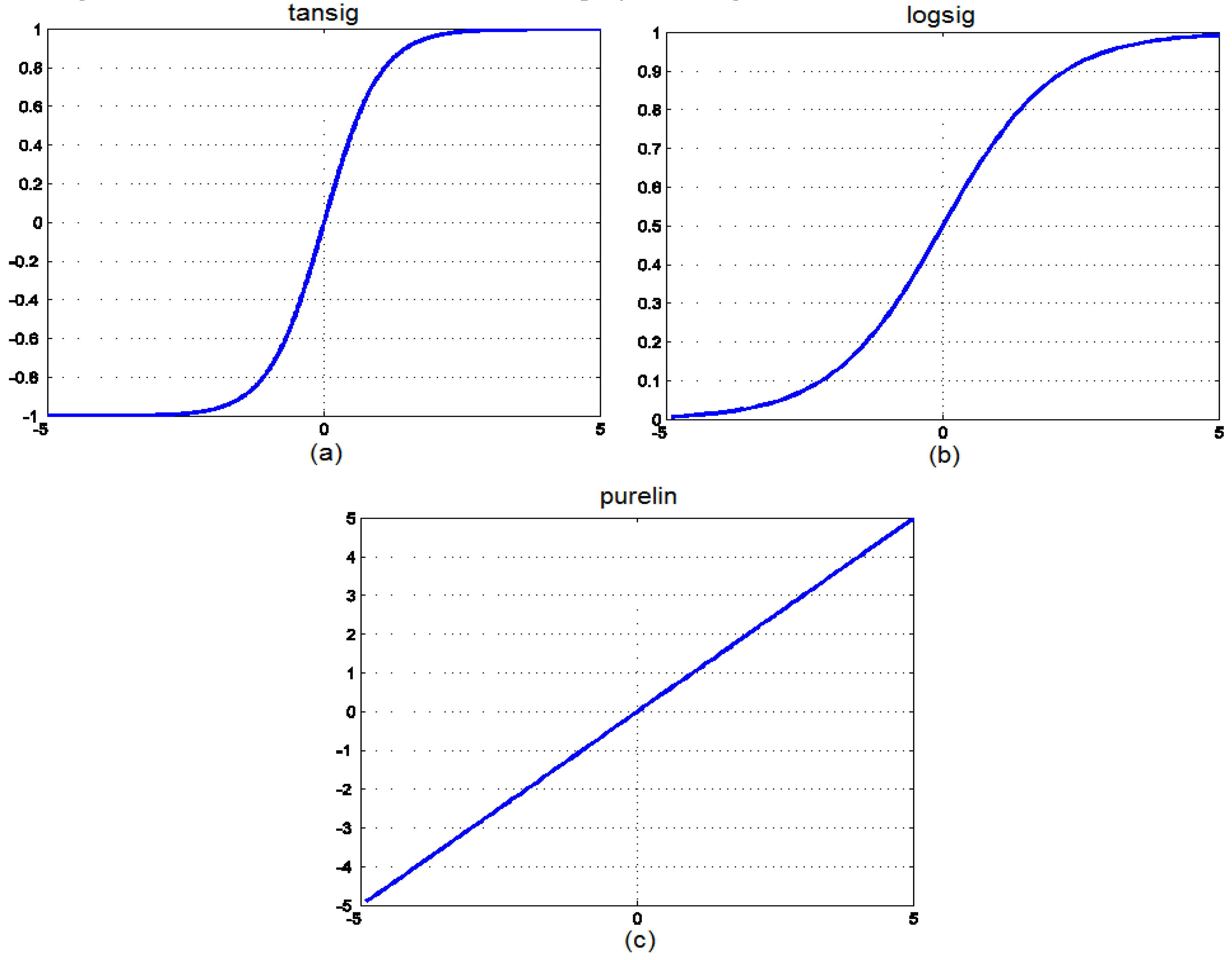
In the above equation, (N) is the number of tested samples; (ti) represents the neural network outputs; and (ai) represents the actual and available outputs. For more information on all types of activation functions, in the MATLAB software, three activation functions—a sigmoid tangent, a sigmoid log function and a linear function—are displayed in Figure 1.
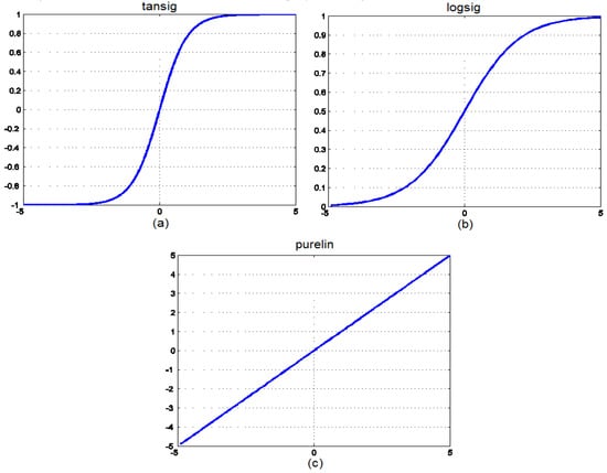
Figure 1.
(a) Sigmoid tangent; (b) sigmoid log function; and (c) purelin function charts.
3.1. Control Systems
After expressing the structure and genetic algorithm, in this section our intention was to use a powerful optimization method to train the neural network and extract the controller PID parameters. First, we explain the structure of the PID controller.
3.1.1. Expression of the Performance of Classical PID Controllers
Control systems are available in both open loop control and closed loop control methods. Both methods of control depend on the system architecture and the control method used for that architecture. Control systems with feedback can be divided into two types. The first of these is single-input and single-output systems, and the second one is the multi-input and multi-output control systems, often referred to as multi-variable control systems.
Open-Loop Control Systems
A loop control system is designed to produce an optimal output value without receiving a feedback system. In this case, the reference signal is given to the actuator and the actuator controls the process. Figure 2 shows the structure of such a control system.

Figure 2.
Open-loop control systems.
Closed Loop Control Systems
In closed loop control systems, the difference between the actual output and the desired output is sent to the controller, and this difference is often amplified and is known as an error signal. The structure of such a control system is shown in Figure 3.

Figure 3.
Closed loop control system.
Multi-Input, Multi-Output Control Systems
By increasing the complexity of the control systems as well as increasing the number of control variables, it was necessary to use the structure of a multi-variable control system, which is the same as shown in Figure 4.

Figure 4.
Multi-input and multi-output control systems.
Proportional–Integral–Derivative Control (PID)
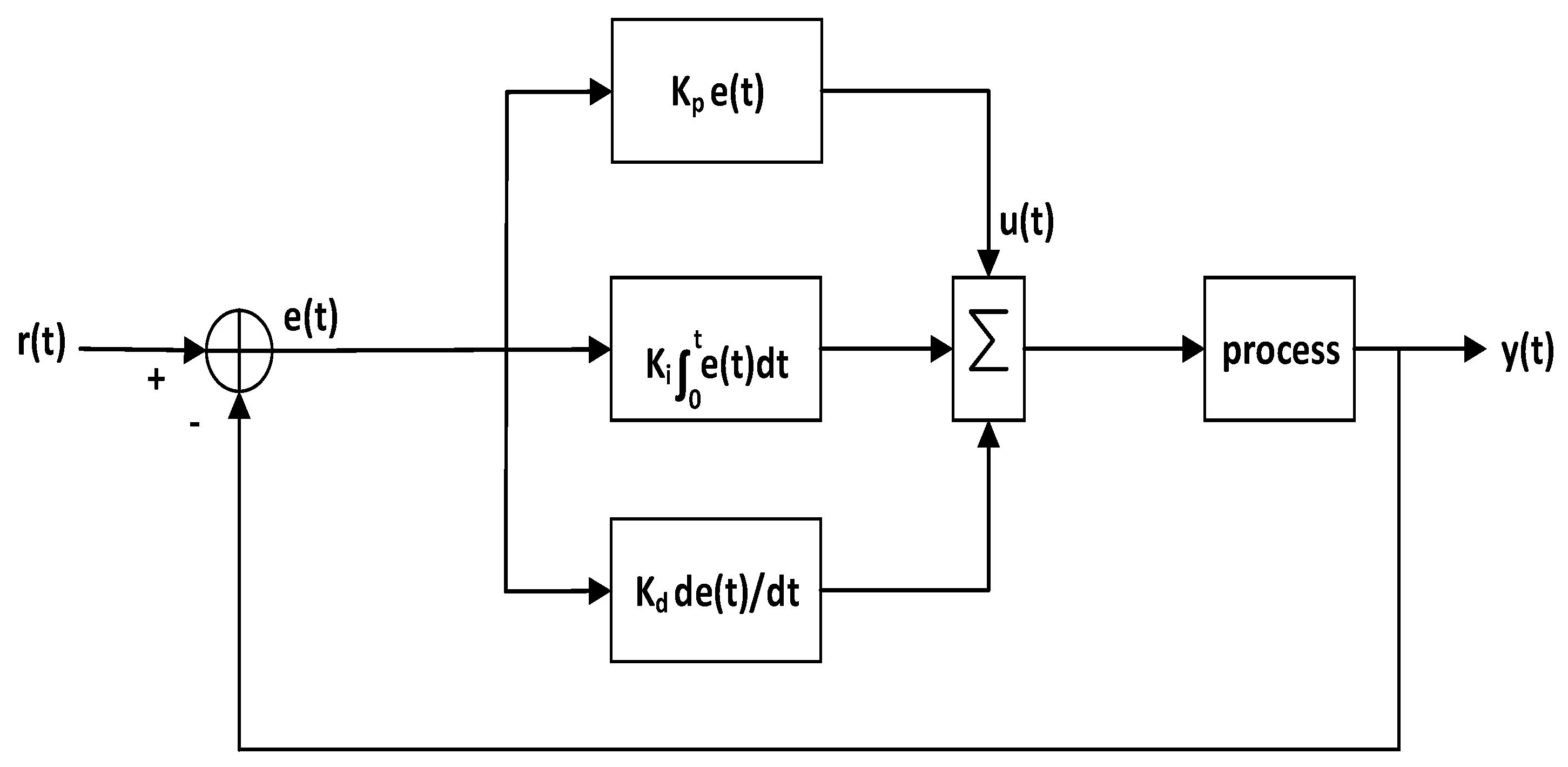
The PID control logic is widely used in controlling industrial processes. Due to the simplicity and flexibility of these controllers, control engineers are using more of them in industrial processes and systems. A PID controller has proportional, integral, and derivative terms, and its transfer function can be represented as Equation (4),
where Kp represents the proportional gain, Ki represents the integral gain, and Kd represents the derivative gain. By adjusting the controller gain, the controller can perform the desired control, which is the same as that shown in Figure 5.

Figure 5.
Closed loop control system with PID controller.
3.2. Neural Network
The structure of the artificial neural network model is inspired by biological neurons. According to the characteristics of biological neurons, we can mention nonlinearity, simplicity of computational units, and learning capabilities. In an artificial neuron, each of the input values is influenced by weight, which is a function of this weight, similar to the synaptic connection in a normal neuron. The processor elements consist of two parts. The first part adds the weighted inputs, and the second part is a non-linear filter called the active function of the neuron. This function compresses the output values of an artificial neuron between asymptotic values. We use multi-layer perceptron with one hidden layer, and inputs of network are derived from error of system. Output of system is controller coefficients, and performance loss function is error from desired value in the next step.
This compression allows the output of the processor elements to remain within a reasonable range. Among the features of artificial neural networks, we can note learning capability, information dispersion, generalizability, parallel processing, and resistance. One of the applications of this type of network is classification, identification and pattern recognition, signal processing, time series prediction, modeling and control, optimization, financial issues, insurance, security, the stock market, and entertainment. Neural networks have the ability to change online; however, in the genetic algorithm, which is essentially an online algorithm, this is not possible. It is normal that if the controller is online, it will provide better answers.
In the design of neural networks, and especially the neural network of delayed time, the designer deals with the problem of selecting the right network for the design. In general, if a network with the least complexity and the minimum parameter has the greatest accuracy in identifying the input patterns, it is called an appropriate network.
A variety of network training is supervised learning, unsupervised learning, and reinforcement learning, which introduce a number of ways of learning in the following:
- (A)
- Perceptron training
For example, the perceptron learning algorithm includes:
- Assigning random values to weights
- Applying the perceptron to each training example
- Ensuring that all training examples have been evaluated correctly [Yes: the end of the algorithm, No: go back to step 2]
- (B)
- Back propagation algorithm
Perceptron have been found in artificial neural network designs, which are characterized by the formation of a multi-layered feed forward structure. The neural synaptic coefficient was configured to be able to estimate ideal processing through the method of back propagation error.
- (C)
- Back-propagation algorithm
To obtain more information on a multi-layer network weight, the back propagation method was conducted by using the gradient descent method to minimize the error square between the outputs of the network and objective function.
The proposed control structure in this designed method is presented as a block diagram of Figure 2 and its control equation is Equation (5):
where u is the controller output in the PID controller designed method using the neural network.
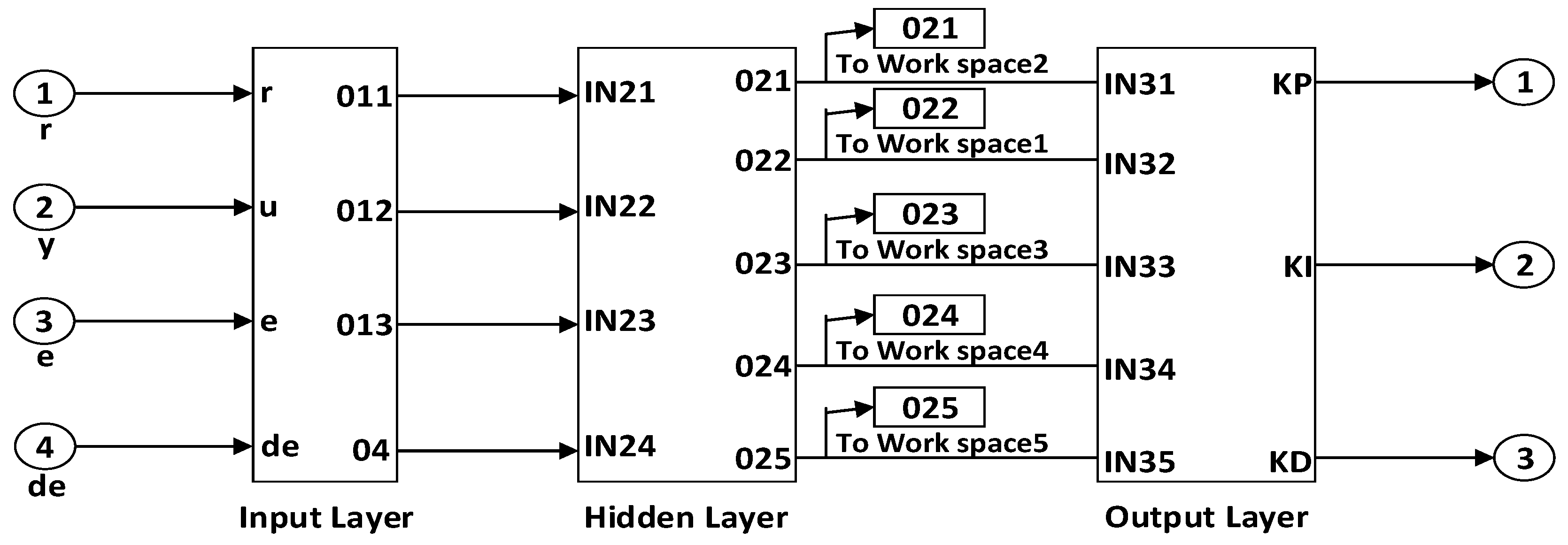
The overall shape of the closed loop structure with the controller and the system conversion function is shown in Figure 6, Figure 7 and Figure 8.
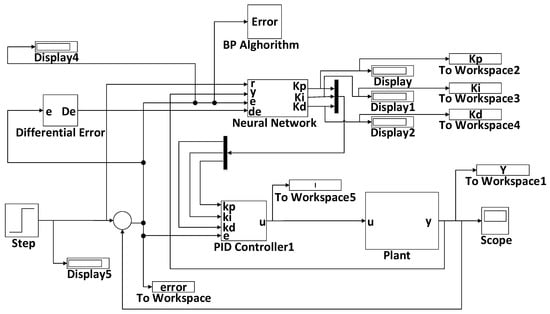
Figure 6.
The structure of the simulinked closed loop with the neural network and the PID controller.

Figure 7.
MLP (Multilayer Perceptron) neural network structure with three layers.
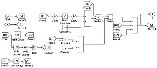
Figure 8.
Plant dynamic structure.
3.3. Genetic Algorithms
We introduce the genetic algorithm optimization method and its basic concepts in this section. The genetic algorithm is an evolutionary solution for optimizing the problem. In the neural network design, we used genetic algorithm to optimize the weights of the neural network. According to the case study, our network is an on-line network that is trained by passing time. The cost function of GA is based on systems error of desired value and this algorithm tries to update weights of neural networks in a manner that the error of desire value reaches the minimum amount.
3.3.1. Genetic Algorithm Optimization Method
The genetic algorithm is based on a biological process to solve optimization problems with and without constraints. The basis of the genetic algorithms work is based on population, which includes the factors of population generation and optimization. In this algorithm, an initial population is generated, then the individuals that have the least amount are selected randomly from the first generated population. The genetic algorithm is an algorithm based on the reproduction process of the creatures. This algorithm is obtained from the generation of chromosomes and chromosomal changes made in the reproduction process and with the production and variation of numbers of chromosomes, the defined interval will try to find an optimal value.
In this method, the first values of the variables are randomly generated as the initial population. Then, by using mutation and intersection, the parents are generated from the initial population, then new numbers are produced as new populations. The population with the initial population is placed in the cost function, and the values are extracted and arranged according to the minimum and maximum values. Finally, after proper algorithmic repetition, the optimal value of the function is extracted. In this section, we deal with the definitions and common terminology in the genetic algorithm as follows:
- Individual: In genetics, each individual is referred to as a member of the population who can participate in the reproduction process and create a new member population that will create an increased population of these individuals.
- Population and production: In genetics, the population is a collection of all individuals that are present in the population, are capable of generating a generation and creating a new one and, consequently, producing a new population.
- Parents: This refers to individuals that intend to participate in the reproduction process and produce a new individual.
3.3.2. The Mathematical Structure of the Genetic Algorithm
Genetic algorithms can be used to solve optimization problems using the following steps:
Step 1: At this stage, an initial population has been created randomly in proportion to the number of variables that optimize its function. After creating the initial population, the function value is calculated for each individual in the first population.
Step 2: In this step, the intersection operation is run to create new chromosomes from the current population in the proceeding step. First, the rate of intersection Pc is chosen (the selection rate was optional) to perform the intersection, then appropriate chromosomes are selected proportional to the rate of the selected intersections before the intersection operation is run according to Equation (6):
In the above equations, V2new and V1new are new chromosomes that have been created by the intersection operation, V2 and V1 are the parent chromosomes, and µ is a random number.
Step 3: In this step, the mutation action is run. First, a random number between zero and one is created according to the size or number of genes in the population (number of genes = population size * number of variables), then the Pm mutation rate is set (the selection of a random value). Then, the mutation action is run according to the following equation where Vknew is a new chromosome that has been caused by mutation action and Xknew is new gene has been altered by mutation action. Equation (7) is:
In Equations (1) and (2), , are the upper and lower borders of , respectively; r is a random number between zero and one; Δ(t, y) with increasing t will tend towards zero; T is the production maximum in the algorithm; and t is the number of production at the moment.
Step 4: In this step, chromosomes in the initial population and chromosomes in the new population in terms of size function based on the values in ascending order are arranged. In proportion to the size of the population, they enter the production cycle. Finally, the minimum function is selected and introduced as the minimum function.
Step 5: The algorithm is a repetition-based algorithm, so the algorithm must be repeated to the maximum desired value so that the function is moved to the optimal point (maximal or minimal) or stop conditions in the algorithm are created.
4. Experimental Result
4.1. Dataset Description
In general, the studies and the results obtained with different numbers of hidden layers for the neural network are summarized in the table below. It is worth mentioning that the chosen training algorithm used a genetic algorithm. Furthermore, the size of the hidden layers in all cases was a single layer. The size of the database was initially 10 samples. As the network was online, the dates changed over time. The criterion for selecting the training and testing data was the lowest error. The number of hidden layers was the layer between the input and output layers. 10 samples are initial samples for training. Then new samples are generated by system as time passes and are used in training. The genetic algorithm selected the best weights that avoided unwanted conditions such as over fitting.
4.2. Optimal Networks Topology
By examining Table 1, it is clear that a hidden layer led to better results. For this reason and to continue the design of the neural network, a number of hidden layers were considered as one layer. In the next step, selecting the best training algorithm for designing a neural network is considered.

Table 1.
Consideration of the results of the neural network with a different number of hidden layers.
According to different training algorithms in MATLAB software, neural network training is considered with two hidden layers. The activator function that is used in the hidden layers in all tested networks, is the tansig activation function. The activation function of the output layer is also considered as the linear.
According to the results presented in Table 2, the best training method for the existing data was the training method with the genetic algorithm. Therefore, the training algorithm was finally considered as the genetic algorithm. In the next step, the choice of the desired neural network parameters, the types of activator functions in the hidden layers as well as the out layer of the designed neural network were considered.

Table 2.
Consideration of the results of testing different training algorithms on the desired neural network.
According to the results shown in Table 3, the lowest error rate and best performance occurred when the activation function on the hidden layer, the logsig type, and the output layer were of the logsig type. The final stage of selecting the neural network parameters was the selection of the size of the hidden layers. By using the results from the previous section, there were two layers with logsig activator functions. Furthermore, the output activator function was the logsig function. Now, by searching for a number of results for different sizes of hidden layers, we reviewed and selected the best available options. In this step, we simulate the system for hidden layers with different size from 1 to 10, and we obtain the results in Table 4.

Table 3.
The results of the consideration of different activator functions in the proposed design of the neural network.

Table 4.
The neural network performance results with different hidden layer size.
According to the results obtained in Table 4, the best solution for the designed neural network occurred when the hidden layer size was 5. It is notable that the proposed method for choosing the best mode for the neural network was merely a local choice, and that it was possible to obtain better results by changing and selecting the parameters out of the range investigated.
4.3. Optimal PID Outputs
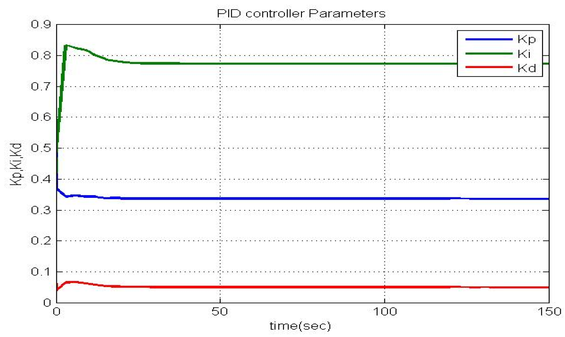
According to the discussion in the previous section, the final designed neural network is as follows. The number of hidden layers of the designed network was considered to be two layers. The hidden layer consisted of a logsig activator function and the output layer of the activator function was also the logsig function. Additionally, the training algorithm was the genetic algorithm. The size of the layers by using the values obtained in the table was 5, therefore there were 5 neurons for the hidden layer. The output waveforms along with the output of the PID controller are shown in Figure 9, Figure 10, Figure 11 and Figure 12.
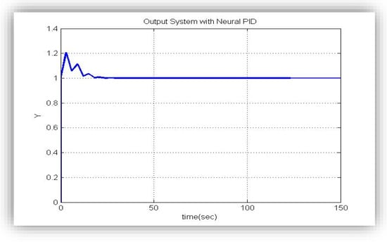
Figure 9.
Output of the controlled system with the PID controller designed with the neural network.
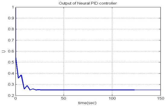
Figure 10.
PID controller output was designed with the neural network and genetic training.
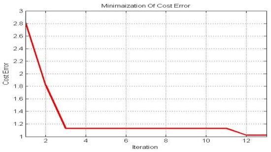
Figure 11.
Minimization chart of the objective function (sum of squared errors) by the genetic algorithm.
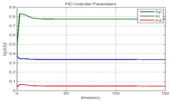
Figure 12.
Convergence of the PID controller parameters designed by the neural network.
As we can see in Figure 11, the objective function was the sum of the squares of the error. The objective function had some defects that, consequently caused the over mutation in the transient response of the system. To solve this problem, the objective function, in terms of the sum of the squares of the error plus the weight function of the over mutation, was chosen as Equation (8).
The output waveform of the closed-loop system with the genetic algorithm training in comparison with the BP algorithm is shown in Figure 13 and Figure 14.

Figure 13.
The output waveform of the controlled system with controllers designed by the neural networks BPNN (Back Propagation Neural Network) and GANN (Genetic Algorithm coupled with Neural Network).
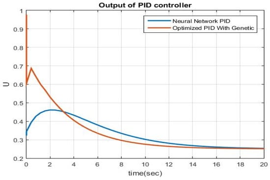
Figure 14.
Neural network controller outputs designed by BPNN and GANN.
5. Conclusions
In this paper, we discussed the design of a PID controller with a neural network and the use of genetic algorithms for an air conditioning system. First, the modeling of the air conditioning system was carried out. At this stage, based on the available information, the system equations were obtained. In the second stage, a discussion about the PID controller and how to determine its coefficients was completed. After that, we examined the neural networks and how to determine the PID controller coefficients with this method. Different conditions for the neural network were considered, and in these conditions, we examined the designed network. Finally, we determined the best network, which has the lowest operating system error criterion.
Out of all of the training algorithms, the genetic algorithm was selected to most effectively train the neural network according to the obtained results. The objective function was minimized by the genetic algorithm, and the sum of the squares of errors was considered to be defective. These defects caused an over mutation in the transient response system. To solve this problem, the objective function was defined as the sum of the squares of error plus the over mutation weighting function. By defining the appropriate cost function, we tried to obtain values that were acceptable with a high ratio. Finally, by simulating a final controlled system, we examined the system response, control signal, and compared the results of the trained neural network with the back propagation algorithm. By comparing the results, it could be seen that the proposed method had advantages over other methods such as the back-propagation algorithm.
Author Contributions
The authors contributed equally to the reported research and writing of the paper. All authors have read and approved the final manuscript.
Conflicts of Interest
The authors declare no conflict of interest.
References
- Winter, R.; Widrow, B. MADALINE RULE II: A training algorithm for neural networks (PDF). In Proceedings of the IEEE International Conference on Neural Networks, San Diego, CA, USA, 24–27 July 1988; pp. 401–408. [Google Scholar]
- Waibel, A.; Hanazawa, T.; Hinton, G.; Shikano, K.; Lang, K.J. Phoneme Recognition Using Time-Delay Neural Networks. IEEE Trans. Acoust. Speech Signal Process. 1989, 37, 328–339. [Google Scholar] [CrossRef]
- Krauth, W.; Mezard, M. Learning algorithms with optimal stabilty in neural networks. J. Phys. A Math. Gen. 2008, 20, L745–L752. [Google Scholar] [CrossRef]
- Guimarães, J.G.; Nóbrega, L.M.; da Costa, J.C. Design of a Hamming neural network based on single-electron tunneling devices. Microelectron. J. 2006, 37, 510–518. [Google Scholar] [CrossRef]
- Mui, K.W.; Wong, L.T. Evaluation of neutral criterion of indoor air quality for air-conditioned offices in subtropical climates. Build. Serv. Eng. Res. Technol. 2007, 28, 23–33. [Google Scholar] [CrossRef]
- ASHRAE. Design for Acceptable Indoor Air Quality; ANSI/ASHRAE Standard 62-2007; American Society of Heating, Refrigerating and Air-Conditioning Engineers, Inc.: Atlanta, GA, USA, 2007. [Google Scholar]
- Levermore, G.J. Building Energy Management Systems: An Application to Heating and Control; E & FN Spon: London, UK; New York, NY, USA, 1992. [Google Scholar]
- Rahmati, V.; Ghorbani, A. A Novel Low Complexity Fast Response Time Fuzzy PID Controller for Antenna Adjusting Using Two Direct Current Motors. Indian J. Sci. Technol. 2018, 11. [Google Scholar] [CrossRef]
- Dounis, A.I.; Bruant, M.; Santamouris, M.J.; Guarracino, G.; Michel, P. Comparison of conventional and fuzzy control of indoor air quality in buildings. J. Intell. Fuzzy Syst. 1996, 4, 131–140. [Google Scholar]
- Tan, W. Unified tuning of PID load frequency controller for power systems via IMC. IEEE Trans. Power Syst. 2010, 25, 341–350. [Google Scholar] [CrossRef]
- Howell, M.N.; Best, M.C. On-line PID tuning for engine idle-speed control using continuous action reinforcement learning automata. Control Eng. Pract. 2000, 8, 147–154. [Google Scholar] [CrossRef]
- European Union. The New Directive on the Energy Performance of Buildings, 3rd ed.; European Union: Brussels, Belgium, 2002. [Google Scholar]
- Tian, L.; Lin, Z.; Liu, J.; Yao, T.; Wang, Q. The impact of temperature on mean local air age and thermal comfort in a stratum ventilated office. Build. Environ. 2011, 46, 501–510. [Google Scholar] [CrossRef]
- Hui, P.S.; Wong, L.T.; Mui, K.W. Feasibility study of an express assessment protocol for the indoor air quality of air conditioned offices. Indoor Built Environ. 2006, 15, 373–378. [Google Scholar] [CrossRef]
- The American Society of Heating, Refrigerating and Air-Conditioning Engineers (ASHRAE). Thermal Environment Conditions for Human Occupancy; ASHRAE Standard 55: Atlanta, GA, USA, 2004. [Google Scholar]
- Wyon, D.P. The effects of indoor air quality on performance and productivity. Indoor Air 2004, 14, 92–101. [Google Scholar] [CrossRef] [PubMed]
- Fanger, P.O. What is IAQ. Indoor Air 2006, 16, 328–334. [Google Scholar] [CrossRef] [PubMed]
- Lundgren, K.; Kjellstrom, T. Sustainability Challenges from Climate Change and Air Conditioning Use in Urban Areas. Sustainability 2013, 5, 3116–3128. [Google Scholar] [CrossRef]
- Maerefat, M.; Omidvar, A. Thermal Comfort; Kelid Amoozesh: Tehran, Iran, 2008; pp. 1–10. [Google Scholar]
- Tian, L.; Lin, Z.; Liu, J.; Wang, Q. Experimental investigation of thermal and ventilation performances of stratum ventilation. Build. Environ. 2011, 46, 1309–1320. [Google Scholar] [CrossRef]
- Morovat, N. Analysis of Thermal Comfort, Air Quality and Energy Consumption in a Hybrid System of the Hydronic Radiant Cooling and Stratum Ventilation. Master’s Thesis, Department of Mechanical Engineering, Tarbiat Modares University, Tehran, Iran, 2013. [Google Scholar]
- Protopapadakis, E.; Schauer, M.; Pierri, E.; Doulamis, A.D.; Stavroulakis, G.E.; Böhrnsen, J.; Langer, S. A genetically optimized neural classifier applied to numerical pile integrity tests considering concrete piles. Comput. Struct. 2016, 162, 68–79. [Google Scholar] [CrossRef]
- Oreski, S.; Oreski, G. Genetic algorithm-based heuristic for feature selection in credit risk assessment. Expert Syst. Appl. 2014, 41, 2052–2064. [Google Scholar] [CrossRef]
- Ghamisi, P.; Benediktsson, J.A. Feature selection based on hybridization of genetic algorithm and particle swarm optimization. IEEE Geosci. Remote Sens. Lett. 2015, 12, 309–313. [Google Scholar] [CrossRef]
- Wang, S.; Jin, X. Model-based optimal control of VAV air-conditioning system using genetic algorithms. Build. Environ. 2000, 35, 471–487. [Google Scholar] [CrossRef]
- Maerefat, M.; Morovat, N. Analysis of thermal comfort in space equipped with stratum ventilation and radiant cooling ceiling. Modares Mech. Eng. 2013, 13, 41–54. [Google Scholar]
- Yu, B.F.; Hu, Z.B.; Liu, M. Review of research on air conditioning systems and indoor air quality control for human health. Int. J. Refrig. 2009, 32, 3–20. [Google Scholar] [CrossRef]
- Yang, S.; Wu, S.; Yan, Y.Y. Control strategies for indoor environment quality and energy efficiency—A review. Int. J. Low-Carbon Technol. 2015, 10, 305–312. [Google Scholar]
- Mui, K.W.; Wong, L.T.; Hui, P.S.; Law, K.Y. Epistemic evaluation of policy influence on workplace indoor air quality of Hong Kong in 1996–2005. Build. Serv. Eng. Res. Technol. 2008, 29, 157–164. [Google Scholar] [CrossRef]
- Chen, S.; Cowan, C.F.N.; Grant, P.M. Orthogonal Least Squares Learning Algorithm for Radial Basis Function Networks. IEEE Trans. Neural Netw. 2010, 2, 302–309. [Google Scholar] [CrossRef] [PubMed]
© 2018 by the authors. Licensee MDPI, Basel, Switzerland. This article is an open access article distributed under the terms and conditions of the Creative Commons Attribution (CC BY) license (http://creativecommons.org/licenses/by/4.0/).

